Receptor modelling of both particle composition ... - Atmos. Chem. Phys

Atmos. Chem. Phys., 15, 10107–10125, 2015 www.atmos-chem-phys.net/15/10107/2015/ doi:10.5194/acp-15-10107-2015 © Author(s) 2015. CC Attribution 3.0 License.

Receptor modelling of both particle composition and size distribution from a background site in London, UK D. C. S. Beddows1 , R. M. Harrison1,3 , D. C. Green2 , and G. W. Fuller2 1 National

Centre for Atmospheric Science School of Geography, Earth and Environmental Sciences, University of Birmingham, Edgbaston, Birmingham B15 2TT, UK 2 MRC PHE Centre for Environment and Health, King’s College London, Franklin-Wilkins Building, 150 Stamford Street, London SE1 9NH, UK 3 Department of Environmental Sciences/Center of Excellence in Environmental Studies, King Abdulaziz University, P.O. Box 80203, Jeddah, 21589, Saudi Arabia Correspondence to: R. M. Harrison ([email protected]) Received: 21 November 2014 – Published in Atmos. Chem. Phys. Discuss.: 2 April 2015 Revised: 27 July 2015 – Accepted: 6 August 2015 – Published: 9 September 2015

Abstract. Positive matrix factorisation (PMF) analysis was applied to PM10 chemical composition and particle number size distribution (NSD) data measured at an urban background site (North Kensington) in London, UK, for the whole of 2011 and 2012. The PMF analyses for these 2 years revealed six and four factors respectively which described seven sources or aerosol types. These included nucleation, traffic, urban background, secondary, fuel oil, marine and non-exhaust/crustal sources. Urban background, secondary and traffic sources were identified by both the chemical composition and particle NSD analysis, but a nucleation source was identified only from the particle NSD data set. Analysis of the PM10 chemical composition data set revealed fuel oil, marine, non-exhaust traffic/crustal sources which were not identified from the NSD data. The two methods appear to be complementary, as the analysis of the PM10 chemical composition data is able to distinguish components contributing largely to particle mass, whereas the number particle size distribution data set – although limited to detecting sources of particles below the diameter upper limit of the SMPS (604 nm) – is more effective for identifying components making an appreciable contribution to particle number. Analysis was also conducted on the combined chemical composition and NSD data set, revealing five factors representing urban background, nucleation, secondary, aged marine and traffic sources. However, the combined analysis appears not to offer any additional power to discriminate sources above that of the aggregate of the two separate PMF analyses. Day-

of-the-week and month-of-the-year associations of the factors proved consistent with their assignment to source categories, and bivariate polar plots which examined the wind directional and wind speed association of the different factors also proved highly consistent with their inferred sources. Source attribution according to the air mass back trajectory showed, as expected, higher concentrations from a number of source types in air with continental origins. However, when these were weighted according to their frequency of occurrence, air with maritime origins made a greater contribution to annual mean concentrations.

1

Introduction

Airborne particulate matter (PM) is recognised as a major public health concern across the EU, with costs estimated at EUR 600 billion in 2005 (Official Journal of the European Union, 2008). In the UK alone, the annual health costs attributable to pollution by airborne PM were estimated in 2007 at between GBP 8.5 billion and 18.6 billion (Defra, 2010). PM exposure was also estimated to reduce people’s lives by on average 7 to 8 months, and by as much as 9 years for vulnerable residents, such as those with asthma, living in pollution hotspots (Environmental Audit Committee, 2010). There is overwhelming evidence that both short-term and long-term exposure to ambient particulate matter in out-

Published by Copernicus Publications on behalf of the European Geosciences Union.

10108

D. C. S. Beddows et al.: Receptor modelling of both particle composition and size distribution

door air is associated with mortality and morbidity (Pope and Dockery, 2006). Source apportionment of airborne particulate matter has assumed increasing importance in recent years, driven by two underlying causes. Firstly, legislative pressure to reduce airborne concentrations of particulate matter has highlighted the need for reliable quantitative knowledge of the source apportionment of particulate matter in order to devise costeffective abatement strategies. The use of source inventories alone is inadequate, as these are limited in the components which they are able to quantify reliably but take no account of the different ground-level impacts of pollutants released at different altitudes or those altered by chemical transformations within the atmosphere. Some sources, such as wood burning, particle resuspension and cooking are very difficult to quantify. Consequently, there has been a need for the application of methods capable of source apportionment of ground-level concentrations. Secondly, there has been growing recognition that abatement of PM mass concentrations, taking no account of source, chemical composition or particle size, may not be a cost-effective approach if the health impact of particulate matter differs according to its source of emissions or physico-chemical characteristics. Consequently, a number of recent epidemiological studies have attempted to combine receptor modelling results with time series studies of health effects (e.g. Thurston et al., 2005; Mostofsky et al., 2012; Ostro et al., 2011). Source apportionment methodology for particulate matter can use either receptor modelling methods or the combination of emissions inventories and dispersion modelling. The latter approach has major weaknesses associated with it, especially regarding the inadequacy of emission inventories referred to above. Consequently, most studies have been based upon receptor modelling methods, and the majority of these have used multivariate statistical methods rather than the chemical mass balance (CMB) model approach (Viana et al., 2008). The multivariate statistical approaches to source apportionment depend upon the fact that different particle sources have characteristic chemical profiles which undergo only modest changes during atmospheric transport from source to the receptor site. Such methods are also able to recognise the contributions of major secondary atmospheric constituents as a result of their characteristic chemical composition. This has led to such methods being widely used for the estimation of contributions to the mass of particles expressed as either PM10 or PM2.5 (Viana et al., 2008; Belis et al., 2013). In addition to having characteristic chemical profiles, air pollutant source categories are also likely to have characteristic particle size distributions which can also be utilised for source apportionment, although these have been utilised rather infrequently in comparison to multi-component chemical composition data. One of the few available studies (Harrison et al., 2011) used a wide range of particle size data collected on Marylebone Road, London, to apportion particuAtmos. Chem. Phys., 15, 10107–10125, 2015

late matter to a total of 10 sources, 4 of which arose from the adjacent major highway. That study also used information on traffic flow according to vehicle type, meteorological factors, and concentrations of gaseous air pollutants as input data, but did not have chemical composition data available derived from simultaneous sampling of airborne particles. Other studies which have used number size distributions (NSDs) with chemical composition for source apportionment include Pey et al. (2009) and Cusack et al. (2013), working in Barcelona. Also in Barcelona, Dall’Osto et al. (2012) applied clustering techniques to NSDs to identify potential sources. Such approaches are likely to be more effective close to particle sources, due to evolution of particle size distributions during atmospheric transport (Beddows et al., 2014). One area of importance of source apportionment of airborne particulate matter arises from the fact that there are most probably differences in the toxicity of particles according to their chemical composition and size association, and, as a consequence, particles from different sources may have a very different potency in affecting human health (Harrison and Yin, 2000; Kelly and Fussell, 2012). There have been many studies of health effects, of which a number have recently incorporated receptor modelling methods and have sought to differentiate between the effects of different source categories on human health. Most have provided some positive and often statistically significant associations with given source factors, chemical components or size fractions (Thurston et al., 2005; Mostofsky et al., 2012; Ostro et al., 2011), but to date there is no coherence between the results of different studies and there is no generally agreed ranking in the toxicity of particles from different sources (WHO, 2013). Consequently, in this context, source apportionment methodology is tending to run ahead of epidemiology and is providing the tools for source apportionment which, thus far, epidemiological research has yet to utilise fully. Nonetheless, work needs to continue towards embedding source apportionment studies in epidemiological research so as to provide clearer knowledge on the toxicity of particles from different sources, or with differing chemical composition and size association. Perhaps the most substantial variations in airborne particle properties relate to their size association, which covers many orders of magnitude. In this context, it is perhaps surprising that toxicity (expressed as effect per interquartile concentration range) appears to be of a broadly comparable magnitude for PM10 mass, which is determined largely by accumulation-mode and coarse-mode particles, and particle number, which reflects mainly nucleation-mode particles. Some studies, however, have suggested different health outcomes associated with the different particle metrics (e.g. Atkinson et al., 2010). In this study, we have applied receptor modelling methods to simultaneously collected chemical composition and particle NSD data from a background site within central London (North Kensington). Our study has initially analysed the www.atmos-chem-phys.net/15/10107/2015/

D. C. S. Beddows et al.: Receptor modelling of both particle composition and size distribution chemical composition and particle NSD data sets separately followed by analysis of the combined data set to test whether this provides advantages in terms of greater capacity to distinguish between source categories.

2 2.1

Experimental Sampling site

The London North Kensington site (lat 51◦ 310 15.78000 N, long 0◦ 120 48.57100 W) is part of both the London Air Quality Network and the national Automatic Urban and Rural Network and is owned and part-funded by the Royal Borough of Kensington and Chelsea. The facility is located within a self-contained cabin within the grounds of Sion-Manning RC Girls’ School. The nearest road, St Charles Square, is a quiet residential street approximately 5 m from the monitoring site, and the surrounding area is mainly residential. The nearest heavily used roads are the B450 (∼ 100 m east) and the very busy A40 (∼ 400 m south). For a detailed overview of the air pollution climate at North Kensington, the reader is referred to Bigi and Harrison (2010). 2.2

Data

For this study, 24 h air samples were taken daily over a 2-year period (2011 and 2012) using a Thermo Partisol 2025 sampler fitted with a PM10 size selective inlet. These were analysed for numerous chemical components listed in Table 1. For total metals (prefixed by the letter T: Al, Ba, Ca, Cd, Cr, Cu, Fe, K, Mg, Mo, Na, Ni, Pb, Sn, Sb, Sr, V, and Zn), the concentration measured using a Perkin Elmer/Sciex ELAN 6100DRC following HF acid digestion of GN-4 Metricel membrane filters is reported. Similarly, all water-soluble ions − − (prefixed by the letter W: Ca2+ , Mg2+ , K, NH+ 4 , Cl , NO3 2− and SO4 ) were measured using a near-real-time URG9000B (hereafter URG) ambient ion monitor (URG Corp). Data capture over the 2 years ranged from 48 to 100 % as different sampling instruments varied in reliability and the metrics analysed. The ions had the lowest data capture rates: WK (48 %), WCA (53 %), WMG (52 %), WNH4 (50 %) and WCL (68 %). This was due to the URG not being installed until February 2011 and experiencing several periods when it malfunctioned either completely or partially – the latter resulting in poor chromatography and the loss of some but not all of the ions. The data capture from the URG independently ranged between 48 % for WK and 68 % for WCL. Daily PM10 filter samples were collected continuously at this site using a Partisol 2025, and laboratory-based ion chromatography measurements were made for anions on Tissuquartz™ 2500 QAT-UP filters sampled between 6 January and 21 October 2011; these were used to fill gaps in the URG data for this period and increased the data capture for the anions. No cation measurements were available from these filters, and www.atmos-chem-phys.net/15/10107/2015/

10109

this resulted in the lower data capture for the cations. All missing data were replaced using a value calculated using the method of Polissar et al. (1998). A woodsmoke metric, CWOD, was also included. This was derived as PMWoodsmoke 10 from the methodology of Sandradewi et al. (2008) utilising Aethalometer and EC/OC data, as described in Fuller et al. (2014). Samples were collected using a Partisol 2025 with a PM10 size selective inlet and concentrations of elemental carbon (EC) and organic carbon (OC) were measured by collection on quartz filters (Tissuquartz™ 2500 QAT-UP) and analysis using a Sunset Laboratory thermal–optical analyser according to the QUARTZ protocol (which gives results very similar to EUSAAR 2: Cavalli et al., 2010) (NPL, 2013). Alongside the composition measurements, number size distribution (NSD) data were collected continuously every 1/4 h using a scanning mobility particle sizer (SMPS) consisting of a CPC (TSI model 3775) combined with an electrostatic classifier (TSI model 3080). The inlet air was dried according to the EUSAAR protocol (Wiedensohler et al., 2012) and the particle sizes covered 51 size bins ranging from 16.55 to 604.3 nm. The data capture of NSD over the 2 years was 72.5 %. In addition, particle mass was determined on samples collected on Teflon-coated glass fibre filters (TX40HI20WW) with a Partisol sampler and PM10 size-selective inlet. 2.3

Positive matrix factorisation

Positive matrix factorisation (PMF) is a well-established multivariate data analysis method used in the field of aerosol science. PMF can be described as a least-squares formulation of factor analysis developed by Paatero (Paatero and Tapper, 1994). It assumes that the ambient aerosol X (represented by a matrix of n × observations and m × PM10 constituents or NSD size bins), measured at one or more sites can be explained by the product of a source matrix F and contribution matrix G, whose elements are given by Eq. (1). The residuals are accounted for in matrix E, and the two matrices G and F are obtained by an iterative minimisation algorithm. xij =

p X

gij · fhj + eij

(1)

h=1

It is commonly understood that PMF is a descriptive model, and there is no objective criterion with which to choose the best solution (Paatero et al., 2002). This work is no exception, and the number of factors and settings for the data sets were chosen using metrics used by Lee et al. (1999) and Ogulei et al. (2006a, b). A detailed description of PMF and our analysis is provided in the Supplement.

Atmos. Chem. Phys., 15, 10107–10125, 2015

EC

Atmos. Chem. Phys., 15, 10107–10125, 2015

TCA

TMG

TZN

Marine

Secondary

Non−Exhaust and Traffic / Crustal

Fuel Oil

1.5

Traffic

0.75

0.5

0.25

0

1

0.75

0.5

0.25

0

0.3 1

0.75

0.2 0.5

0.1 0.25

0.0 0

0.15 1

0.75

0.10 0.5

0.05 0.25

0.00 0

0.3 1

0.75

0.2 0.5

0.1 0.25

0.0 0

1

1.0

0.75

0.5

0.5

0.25

0.0

0

Explained Variation

1

Explained Variation

TMG

TZN

TV

TTI

Urban Background

Explained Variation

TMG

TZN

TV

TTI

TSB

TPB

Marine

Traffic

Fuel Oil

Non−Exhaust Traffic and Crustal

Secondary

[µg/m3]

Concentration

Urban Background

Traffic

Fuel Oil

Non−Exhaust Traffic and Crustal

4

Explained Variation

TMG

TZN

TV

TTI

TSB

TPB

TNI

TNA

TMO

Marine Secondary

6

Explained Variation

TMG

TZN

TV

TTI

TSB

TPB

TNI

TNA

TMO

TMN

TK

TFE

Urban Background

8

Explained Variation

TMG

TZN

TV

TTI

TSB

TPB

0.4

TV

TTI

TSB

TPB

TNI

TNA

TMO

TMN

TK

TFE

TCA TCU

[µg/m3]

Concentration

Sun Mon Tue Wed Thu Fri Sat

TSB

TNI

TNA

TMO

TMN

TK

TFE

TCA TCU

TAL TBA

Average Week

TPB

TNI

TNA

TMO

TMN

TK

TFE

TCA TCU

TAL TBA

WCL WNH4

5 4 3 2 1 0

TNI

TNA

TMO

TMN

TK

TFE

TCA TCU

TAL TBA

WNH4

17.2 µg m3

TMN

TK

TFE

TCA TCU

TAL TBA

WNH4

WSO4

%

TCU

TAL TBA

WNH4

WCL

Traffic 4.5%

TBA

WNH4

WCL

WNO3

CWOD

Non−Exhaust and Crustal 25.1%

TAL

WNH4

WCL

WSO4

WNO3

CWOD

5.1

WCL

WSO4

WNO3

CWOD

EC OC

e1

WCL

WSO4

WNO3

CWOD

EC OC

rin

WSO4

WNO3

CWOD

EC OC

Weight within Factor (no units)


Ma

WSO4

WNO3

EC OC


Urban Background 24.0%

CWOD

EC OC

Weight within Factor (no units) 0.30 0.25 0.20 0.15 0.10 0.05 0.00

OC


.9%

0.30 0.25 0.20 0.15 0.10 0.05 0.00 il 5 el O

Secondary 25.4%

Fu


10110 D. C. S. Beddows et al.: Receptor modelling of both particle composition and size distribution

Average Year Jan Mar Jun Sep Dec

2

0

Figure 1. Factors outputted from PMF2 run on PM10 mass composition data showing the contribution (grey bar) and explained variation of each metric (red bar).

www.atmos-chem-phys.net/15/10107/2015/

%

Secondary

0

4.4

5512 cm−3

Nucleation

500

Traffic

1000

Jan Feb Mar Apr May Jun Jul Aug Sep Oct Nov Dec

Urban Background

Concentration [ cm−3]

8%

1500

10111

Average Year

3000 2500 2000 1500 1000 500 0

Nucleation

2 nd ry

2000

Traffic



Urban Background

Nucl. 7.

Average Week

2500

Secondary

Traffic 44.8%



0.00

0.18

0

0.02

0.10

D p [μ m]

0

0.50

5

10

15

Explained Variation

0.20

280

0.16

0.25

0.01

240

0.5

0.02

200

0.75

0.03


0.04

Explained Variation


Secondary 1

20

Hour

0.00

0.365 0.350

2800

0

0.02

0.10

D p [μ m]

0

0.50

5

10

15

20

Explained Variation

0.25

0.01

0.335

0.5

0.02

2400

0.03

2000

0.75

0.04


0.05

Explained Variation


Urban Background 1

Hour

0.25

0.01 0.00

0.30 0.28

Explained Variation

0.02

0.26

0.5

0.03

3000

0.75

0.04

2000

0.05


0.06

Explained Variation


Traffic 1

0

0.02

0.10

D p [μ m]

0

0.50

5

10

15

20

Hour

0.00

0.09

600

0.07

0

0.02

0.10

D p [μ m]

0.50

0

5

10

15

Explained Variation

0.25

0.02

0.05

0.04

400

0.5

0.06

200

0.75

0.08


0.10

Explained Variation


Nucleation 1

0.12

20

Hour

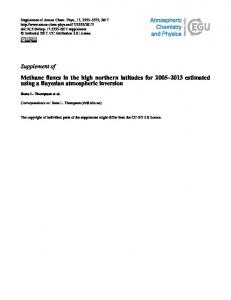
Figure 2. Factors outputted from PMF2 run on the particle number size distribution showing the contribution (black line) and explained variation of each metric (red line).


Atmos. Chem. Phys., 15, 10107–10125, 2015

10112


Table 1. Measurements collected at the North Kensington site, 2011 and 2012.

3

Species

Brief description

PM fraction

Detailed description

TMN TMO TNA TNI TPB TSB TSN TSR TTI TV TZN TAL TBA TCA TCD TCR TCU TFE TK TMG PCNT PM10 PM25 EC OC CWOD

Manganese Molybdenum Sodium Nickel Lead Antimony Tin Strontium Titanium Vanadium Zinc Aluminium Barium Calcium Cadmium Chromium Copper Iron Potassium Magnesium Particle number PM10 PM2.5 Elemental carbon Organic carbon OA Wood burning

PM10

Total metal concentration – HF acid digest and ICPMS

PM1 PM10 PM2.5 PM10 PM10 PM2.5

Condensation particle counter (CPC, TSI) EU reference equivalent; gravimetric with gaps filled from FDMS-TEOM EU reference equivalent; FDMS-TEOM with gaps from gravimetric By thermo-chemical analysis using Sunset instrument and NIOSH TOT protocol

WNO3

Nitrate

PM10

WSO4 WCL WNH4 WCA WMG WK

Sulfate Chloride Ammonium Calcium Magnesium Potassium

OA from wood using Aethalometer; wood-burning model of Sandradewi et al. (2008) as in Fuller et al. (2014) Water-soluble measured using near-real-time URG; gaps filled with filter measurements

Results

The final PMF solutions were selected as those with most physically meaningful profiles. Once the PMF output is chosen and scaled, the values of the F matrix are used to characterise the source term. Each row i of F represents a source, and each element fhj shows the “weight within the factor” (WWTF) of the constituent (grey bars and black NSD lines in Figs. 1 to 3). Together with the dimensionless F matrices, a matrix due to Paatero, called the explained variation (EV) shows how much of the variance in the original data set is accounted for by each factor (again see the Supplement for more details). For a given column (PM component measurement or particle size bin) of the total EV matrix, the total EV (TEV) is recommended to be 0.75 or greater. Although a useful metric in assessing the ability of the final PMF settings to model the data, high EV values (red bars or NSD line in Atmos. Chem. Phys., 15, 10107–10125, 2015

Figs. 1 and 2) indicate which sources are the most important source for each constituent and hence significantly aid factor identification when considered alongside the WWTF. The Gi matrix gives the contribution of the source terms Fi and carries the original units of X. The values within the columns of matrix G contain the hourly/daily contributions made by the p factors (or sources) and are used to calculate the diurnal, weekly and yearly averages (see Figs. 1 to 3). The identity of the source, namely marine, secondary, traffic, nucleation, etc., was assigned on the basis of post hoc comparison with known source profiles, tracers (Viana et al., 2008), physical properties and temporal behaviour.



2

D p [µm]

0.6

0.5

0.4

0.3

0.2

0.1

0.08 0.09

0

Traffic 1

8 6 4 2 0

0.75 0.5 0.25

0.5

0.4

0.6

D p [µm]

0.3

0.2

0

Explained Variation Explained Variation

0.6

0.5

0.4

0.25

Explained Variation

0.6

0.5

0.4

0.3 0.3

0.2

0.1

0.5

Explained Variation

0.6

0.5

0.4

0.3

0.2 0.2

0.1

0.08 0.09 0.08 0.09

0.75

Explained Variation

Traffic

Aged Marine

Secondary

Nucleation

Urban Background

0.1

0.08 0.09

0.07

0.06 0.06

0.07 0.07

1

0.1

F (arbitrary units)

0.06

Aged Marine

EC OC CWOD WNO3 WSO4 WCL WNH4 TAL TBA TCA TCU TFE TK TMN TMO TNA TNI TPB TSB TTI TV TZN TMG

0.30 0.25 0.20 0.15 0.10 0.05 0.00

D p [µm]

8 6 4 2 0


0.00

Traffic

0

0.08 0.09

0.05

0.04

0.25

0

0.07

0.10

0.05

0.5

2

0.06

0.15

0.04

0.75

4

0.02

F (arbitrary units)

0.20

1

6


0.00

Secondary

0.07

0.05

D p [µm]

8

0.06

0.10

0.05

0

0.04

0.15

0.03

0.25

0

0.05

0.20

Aged Marine

Nucleation

0.5

5

0.02

F (arbitrary units)

0.25

Secondary

0.75

10

0.04

0.00

1

15

0.05

0.02

Nucleation

0.04

0.04

D p [µm]

20

0.05

0.06

0

0.02

F (arbitrary units)

0.08

0.25

0.03

0.00

1

EV

0.5

0.03

0.05

0.03

0.10

Volume

0.75

0.03

0.15

NSD

0.02

0.20

Urban Background

NSD 25 20 15 10 5 0

0.02

PM10

0.25

0

0 Urban Background

Aged Marine 16.7%


F (arbitrary units) F (arbitrary units) F (arbitrary units) F (arbitrary units)

4

1

Traffic 15.9%

Jan Feb Mar Apr May Jun Jul Aug Sep Oct Nov Dec

6

G value

2

F (arbitrary units)

0.30

3


F (arbitrary units)

Secondary 21.5%



4

G value

Nucleation 20.0

Average Year

8

Average Week

5

10113

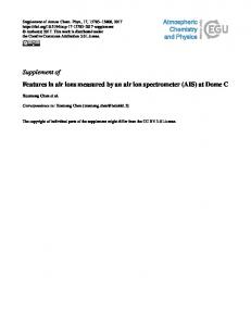
Figure 3. Five-factor solution from the combined composition–NSD data set showing the contribution (black line) and explained variation of each metric (red line).

3.1

The six-factor solution for PM10 chemical composition data

An optimum six factor solution was chosen which best represented the aerosol types. Figure 1 characterises the six factors as urban background, marine, secondary, non-exhaust traffic/crustal, fuel oil and traffic. While most of the names of these factors are self-explanatory, “urban background” has a chemical profile indicative of contributions mainly from both woodsmoke (CWOD) and road traffic (Ba, Cu, Fe, Zn). Since these are ground-level sources which are affected in a similar way by meteorology (see polar plots for the urban www.atmos-chem-phys.net/15/10107/2015/

background and traffic factors in Figs. 4 and 5), PMF is not able to effect a clean separation in 24 h samples, and this problem is exacerbated by the tendency of the Aethalometer – which was used to derive the woodsmoke-associated CWOD variable – to include some traffic-generated carbon in the woodsmoke estimate (Harrison et al., 2013a). In the ClearfLo winter campaign (Clean Air for London, Bohnenstengel et al., 2015), black carbon (traffic) from Aethalometer measurements correlated strongly with the woodsmoke tracer levoglucosan at North Kensington (r 2 = 0.80) (Crilley et al., 2015).

Atmos. Chem. Phys., 15, 10107–10125, 2015

10114

D. C. S. Beddows et al.: Receptor modelling of both particle composition and size distribution Urban Background

Secondary

Marine 8

N

25

7

20 15 wind spd.

N

25 20

15 wind spd.

6

10

5

5 W

E

4

8

20 15 wind spd.

6

10

9

N

25

7

7

10

5

5 W

E

6

5 W

E

4

3

4

3 2

3 2

1 S

S

Non−Exhaust Traffic and Crustal N

25 20

5 E

6

N

25

0.6

15 wind spd.

1

10

10

0.5 5

5 E

W

5 4

0.9

W

E

0.4 0.3

0.8

0.2

3 0.7

2 S

0.7

20

1.1 15 wind spd.

7

W

Traffic

N 20

8

10

2 S

1

Fuel Oil 25

9

15 wind spd.

5

0.1 S

S

1

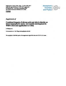
Figure 4. Polar plots showing how the daily PM10 contributions are affected by the daily vector average wind direction and velocity (units: PM10 (µg m−3 ) and wind speed (m s−1 )).

When comparing five-, six- and seven-factor solutions, common sources could be identified in all three solutions, namely urban background, marine, secondary, non-exhaust traffic/crustal, and fuel oil. In the five-factor solution, the urban background factor had elevated values of EC, Ba, Cu, Fe, Mg, Mn and Sb, all of which are indicative of a traffic contribution. By increasing the number of factors from five to six, the concentration of these elements within the urban background factor decreased as a traffic factor separated out into its own unique factor, although a complete separation was not observed even when using seven factors. Furthermore, when using seven and eight factors, the urban background factor remained unaltered and the fuel oil factor was observed to shed a spurious factor containing odd combinations of Ni, Pb, Zn, SO2− 4 , and OC contributions. This led to the conclusion that only six factors yielded a meaningful solution. Considering further the six-factor solution, the marine factor clearly explains much of the variation in the data for Na, Cl− and Mg2+ , and the secondary factor is identified − 2− from a strong association with NH+ 4 , NO3 , SO4 and organic carbon. For the traffic emissions, the PM does not simply reflect tailpipe emissions, as it also includes contributions from non-exhaust sources, including the resuspension of road dust and primary PM emissions from brake, clutch and tyre wear (Thorpe and Harrison, 2008). The non-exhaust traffic/crustal factor explains a high proportion of the variation in the Al, Ca2+ and Ti measurements consistent with particles derived from crustal material, derived either from wind-blown or vehicle-induced resuspension. There is also a significant explanation of the variation in elements such as Zn, Pb, Mn, Fe, Cu and Ba, which have a strong association with non-exhaust traffic emissions. As there is a strong contribution of crustal material to particles resuspended from

Atmos. Chem. Phys., 15, 10107–10125, 2015

traffic (Harrison et al., 2012), it seems likely that this factor is reflecting the presence of particulate matter from resuspension and traffic-polluted soils. The fifth factor, attributed to fuel oil, is characterised by a strong association with V and Ni together with significant SO2− 4 . These are all constituents typically associated with emissions from fuel oil combustion. The sixth factor shows an especially strong association with elements derived from brake wear (Ba, Cu, Mo, Sb) and tyre wear (Zn) (Thorpe and Harrison, 2008; Harrison et al., 2012). This had the highest correlation to BC and was assigned the title of traffic factor. For exhaust from road traffic, the ratio of elemental carbon (EC) and organic carbon (OC) is approximately 2 : 1. This a priori information was applied to the traffic factor by pulling the OC constituent in the factor using an FKEY value of 5. Also shown in Fig. 1 is a pie chart showing the proportion of mass concentration associated with each of the factors, as well as bar charts showing the day-of-the-week dependence and monthly dependence of the average concentration of each factor. Three sources predominate: non-exhaust traffic/crustal (25 %), secondary (25 %) and urban background (24 %), with lesser contributions from marine (15 %), local traffic (5 %) and fuel oil (6 %). Both the traffic and nonexhaust traffic/crustal factors show higher concentrations on weekdays than at weekends, reflecting traffic activity in London. The urban background source shows slightly higher concentrations at weekends, likely to be a reflection of wood burning since measurements of the wood-burning tracer levoglucosan in 2010 were found to be 30 % greater on Saturdays and 54 % greater on Sundays when compared to weekday concentrations (Fuller et al., 2014). The marine and fuel oil factors show no consistent variation with regard to day of the week. In the case of the monthly variations, the ur-


D. C. S. Beddows et al.: Receptor modelling of both particle composition and size distribution SECONDARY

URBAN BACKGROUND

TRAFFIC

NUCLEATION

Figure 5. Polar plots showing how the hourly NSD contributions are affected by the hourly wind direction and wind velocity (units: NSD (cm−3 ) and wind speed (m s−1 )).

ban background, marine, secondary and non-exhaust traffic/crustal sources all show signs of higher concentrations in the cooler months of the year. Both the urban background and traffic-related sources are emitted at ground level and are likely to be less well dispersed in a shallower mixing layer during the colder months of the year. Marine aerosol typically shows a seasonal variation, with elevated concentrations associated with the stronger winds in the winter months. The secondary constituent is particularly strong in the spring, which is when nitrate concentrations are typically elevated (Harrison and Yin, 2008), probably as a result of relatively low air temperatures suppressing the dissociation of ammowww.atmos-chem-phys.net/15/10107/2015/

10115

nium nitrate and increased emissions of ammonia due to the spreading of slurry on farmland. The only constituent to show higher concentrations in the warmer months of the year is the fuel oil source. This might be attributable to emission from high chimneys, with more efficient mixing to ground level during the more convective summer months, or to enhanced sulfate formation due to photochemistry, as this is the largest chemical component of this factor by mass. Polar plot data derived with the Openair program appear in Fig. 4, which is discussed in Sect. 3.4. Figure 6 plots how the factors contributed daily across the 2-year data set to the total measured PM10 , and the vertical dotted lines identify the period containing the highest contribution of each factor to the PM10 mass concentration. Air mass back trajectories corresponding to these periods have been calculated using HYSPLIT (Draxler and Rolph, 2015) and are shown in Fig. 7. As expected, the largest contribution of the marine factor occurred for the long (i.e. high average wind speed) maritime trajectories associated with marine aerosol production. The secondary factor was associated with winds from the European mainland crossing the Benelux countries en route to the North Kensington site. This trajectory sector from London was identified by Abdalmogith and Harrison (2005) as strongly associated with elevated sulfate and nitrate concentrations. The traffic factor was associated with a trajectory travelling across eastern and northern France before crossing the English Channel to the UK, approaching the North Kensington site from the south-east. Such a trajectory is likely to maximise both the long-range-advected contribution and the local contribution within London. The highest contribution from the urban background factor was during the identical period to the highest traffic contribution and hence the identical back trajectories. Examination of Fig. 6 shows many similar features in the time series of the urban background and traffic source categories which confirm the impression that road traffic makes a substantial contribution to the urban background factor. The maximum contribution from the non-exhaust/crustal factor was again on an easterly circulation rather similar to that giving a maximum in the secondary contribution (Fig. 7). This trajectory was likely to include not only a substantial contribution from air advected from mainland Europe but also from air from the centre and east of London. Perhaps most interesting is the trajectory associated with the highest contribution of the fuel oil factor, which shows air arriving predominantly from the English Channel and remaining at low altitude, confirming the impression that there may be a major contribution from shipping to the fuel oil factor. This would be consistent with the observation of Johnson et al. (2014) that shipping was the main source impacting upon V in Brisbane, Australia, and that this was associated with both sulfur and black carbon, and other observations that shipping emissions affect concentrations of V (Pey et al., 2013; Zhao et al., 2013; Minguillon et al., 2014; Viana et al., 2014). In our data shown in Fig. 1, the fuel oil Atmos. Chem. Phys., 15, 10107–10125, 2015

10116

D. C. S. Beddows et al.: Receptor modelling of both particle composition and size distribution Urban Background

30

3.2

The four-factor solution for the number size distribution (NSD) data

20 10 0 Marine

12.5 10.0 7.5 5.0 2.5 0.0

Secondary

Concentration [μ g/m3]

40 30 20 10 0 Non-Exhaust Traffic and Crustal 20 10 0 Fuel Oil

4 3 2 1 0

Traffic 3 2 1 0

12 13 11 12 12 12 11 11 11 5-20 1-08-20 1-11-20 1-02-20 1-05-20 1-08-20 1-11-20 1-02-20 0 0 0 0 0 0 01-0 0

2-20

01-0

date

Figure 6. Daily factor scores outputted from PMF2 GF. Vertical red lines indicate when each factor has the highest contribution to PM10 : 20 November 2011 – urban background; 23 December 2012 – marine; 18 February 2011 – secondary; 21 April 2011 – nonexhaust and crustal; 15 August 2012 – fuel oil; 20 November 2011 – traffic.

factor accounted for almost 75 % of the explained variation of V. Receptor modelling of airborne PM collected in Paris, France, revealed a heavy oil combustion source which accounted for a high percentage of V and Ni, and some SO2− 4 , with a predominant source area around the English Channel (Bressi et al., 2014), consistent with a substantial influence of shipping emissions. Table 2 shows the average concentrations of gas-phase pollutants and meteorological conditions corresponding to the period when each factor in the PMF results for PM10 chemical composition exceeded its 90-percentile value. Notable amongst these are the high CO and NOx concentrations associated with the traffic and urban background sources and the relatively clean air of the marine source.

Atmos. Chem. Phys., 15, 10107–10125, 2015

The PMF analysis of the hourly averaged measurements collected at North Kensington (2011–2012) yielded an optimum four-factor solution. Figure 2 characterises the four factors as secondary, urban background, traffic and nucleation. Comparison of this optimum solution with its counterparts using three and five factors revealed that all three solutions had a traffic and urban background factor in common. Using three factors, the nucleation and secondary factors were combined and only separated when using four factors. When using five factors, the secondary factor divided again, shedding an obscure factor with three modes at ∼ 0.03, ∼ 0.08 and ∼ 0.3 µm, all equally spaced along the log10 (Da ) axis. This spurious factor had a noticeable correlation with its parent factor, suggesting factor splitting at five factors, leading to a conclusion that only four factors could be used to obtain a meaningful solution. Figure 2 also shows the weekday/weekend and seasonal behaviour of these factors, the NSDs associated with each factor and the explained variation for each size bin. The right-hand panels show the diurnal variation of each factor and the variance explained for each time of day. Figure 8 plots how these factors contributed on a daily basis across the 2-year data set to the total NSD measured. The secondary factor shows by far the coarsest particle sizes, with a minimum concentration in the early afternoon likely associated with the evaporation of ammonium nitrate at higher air temperatures and lower relative humidities. There is no consistent day-of-the-week pattern, and elevated concentrations in spring presumably arise for the same reasons as for the PM10 secondary constituent. The traffic factor has a modal diameter at around 30 nm and a large proportion of the variation explained within the main peak of the distribution. The diurnal pattern has peaks associated with the morning and evening rush hour periods, and there are lower concentrations at weekends and higher concentrations in the winter months of the year. All of these features are consistent with emissions from road traffic (Harrison et al., 2011). The factor described as urban background has a modal diameter intermediate between that of the traffic and secondary factors and a diurnal pattern consistent with that expected for traffic emissions. Its concentrations are elevated at weekends, presumably associated with wood burning (as reported by Fuller et al., 2014) and higher concentrations in the cooler months of the year (as noted by Crilley et al., 2015). Both the traffic and urban background factors correlate with black carbon (r = 0.50 and 0.82 respectively), and also with NOx (r = 0.53 and 0.78 respectively). This is strongly suggestive of a major road traffic input to both factors. The fourth factor, which is attributed to nucleation, has by far the smallest particle mode at around 20 nm and peaks around 12:00 in association with peak solar intensities. It shows a seasonal cycle with the highest concentrations on average in the summer www.atmos-chem-phys.net/15/10107/2015/


10117

Figure 7. Back trajectories corresponding to the vertical red lines in Fig. 6, which indicate when each factor has the highest contribution to PM10 : 20 November 2011 – urban background; 23 December 2012 – marine; 18 February 2011 – secondary; 21 April 2011 – non-exhaust and crustal; 15 August 2012 – fuel oil; 20 November 2011 – traffic.

Table 2. Average concentrations of gas-phase pollutants and meteorological conditions corresponding to the periods when each factor in the PMF results for the PM10 chemical and NSD exceeded its 90 percentile value. (WD – wind direction; WS – wind speed; VIS – visibility; P – pressure; T – temperature; DP – dew point; RH – relative humidity.) PM10 Traffic Fuel oil Non-exhaust/crustal Secondary Marine Urban background NSD Secondary Urban background Traffic Nucleation PM10 Traffic Fuel oil Non-exhaust/crustal Secondary Marine Urban background NSD Secondary Urban background Traffic Nucleation


CO mg m−3

NO µg m−3

NO2 µg m−3

NOx µg m−3

O3 µg m−3

SO2 µg m−3

0.43 0.20 0.35 0.28 0.22 0.38

50.02 4.42 26.64 18.09 5.69 42.69

62.59 27.63 53.71 48.79 29.48 61.42

139.05 34.33 94.67 76.61 38.40 126.46

12.42 46.82 24.50 48.65 46.54 20.15

3.71 1.25 3.48 3.23 2.04 3.91

CO mg m−3

NO µg m−3

NO2 µg m−3

NOx µg m−3

O3 µg m−3

SO2 µg m−3

0.38 0.39 0.32 0.24

30.72 44.19 29.70 9.31

57.48 60.43 54.04 33.52

104.63 128.19 99.91 47.88

25.93 23.84 20.63 37.00

3.75 3.58 2.77 2.23

WD degrees

WS m s−1

VIS m

P mbar

◦

T C

DP ◦ C

RH %

196 205 134 152 203 166

4.79 11.25 5.56 6.17 7.84 4.87

1197 2239 951 1687 2085 1405

1022 1015 1023 1019 1015 1020

6.01 11.41 9.09 14.98 16.24 11.33

3.01 6.93 5.37 7.90 11.15 6.64

81.93 75.47 79.33 65.34 73.93 76.54

WD degrees

WS m s−1

VIS m

P mbar

◦

T C

DP ◦ C

RH %

141 168 193 206

5.14 4.67 5.79 7.95

878 1266 1903 2103

1022 1021 1020 1015

10.73 10.64 9.27 12.8

6.33 6.13 5.14 7.9

76.68 76.63 77.51 74.27

Atmos. Chem. Phys., 15, 10107–10125, 2015

10118

D. C. S. Beddows et al.: Receptor modelling of both particle composition and size distribution Secondary

10000 5000 0 Urban Background

Concentration [ cm-3]

3000 2000 1000 0 Traffic 9000 6000 3000

5000

Nucleation

4000 3000 2000 1000 0

11 11 12 12 11 11 12 12 8-20 2-20 1-05-20 2-20 1-05-20 1-20 1-20 8-20 01-0 0 0 01-0 01-0 01-1 01-1 01-0

date

Figure 8. Daily factor scores outputted from PMF2 GF (unit: cm−3 ). Vertical red lines indicate when each factor has the highest daily average contribution to the NSD: 24 March 2012 – secondary; 1 October 2011 – urban background; 27 January 2012 – traffic; 17 July 2012 – nucleation.

months in the second year (Fig. 8) and a preference for weekday over weekend periods. The apparent lack of a seasonal pattern in the first year of observations is surprising. However, nucleation depends upon a complex range of variables including precursor availability, insolation and condensation sink, and the reasons are unclear. The apparent background level of nucleation in the second year accounting for up to 1000 cm−3 particles may be the result of an incomplete separation of this factor from other source-related factors. The mean particle number concentration, measured using the SMPS was 5512 cm−3 , of which traffic and urban background made the highest percentage contribution of 44.8 and 43.0 % respectively, followed by nucleation (7.8 %) and secondary (4.4 %). Figure 8 includes dotted vertical lines which identify the days with the highest average contribution of each factor to the total particle number concentration, and the air mass back trajectories corresponding to these periods have been plotted in Fig. 9. This shows some differences relative to the factors derived from the PM10 composition data set. The secondary factor trajectories originated over the North Sea, and the majority crossed parts of Germany and the Netherlands, on a more northerly path than the trajectories of the PM10 secondary factors. The trajectory for the urban background source had crossed over north-eastern France before arriving at North Kensington in a similar manner to the PM10 urban background trajectory. The traffic factor back trajecAtmos. Chem. Phys., 15, 10107–10125, 2015

tory approached from the west after crossing the southern United Kingdom, which is quite different to the PM10 traffic factor seen in Fig. 7. The nucleation factor was associated with relatively low ocean wind speeds and crossed the southern UK before reaching the sampling site. The nucleation factor is predominantly maritime and therefore likely to bear a rather low aerosol concentration, hence favouring the nucleation process. Table 2 presents the average gas-phase pollutant concentrations and meteorological conditions corresponding to the peak contribution of the various factors. Notable amongst these are the low concentrations of carbon monoxide, oxides of nitrogen, and sulfur dioxide, and the high ozone concentration associated with the nucleation factor. In Table 3 the correlation coefficients are given between the factors derived from the PM10 composition data set and those from the NSD data set. There are moderate correlations between the urban background factors determined from the two PMF analyses and for the secondary factors. The PM10 traffic factor has a higher correlation with the NSD urban background factor than the NSD traffic factor, and the PM10 Urban Background factor shows a very modest correlation with the NSD traffic factor. This serves to confirm the contribution of traffic to the urban background factor. The nucleation factor in the NSD data set and marine and fuel oil factors in the PM10 composition data set do not correlate substantially with factors in the other data set. Figure 10 shows the average clustered trajectories for air masses arriving daily at North Kensington over the 2-year period. Three of the clustered trajectories (2, 4, and 7) are considered as one and representative of an air mass travelling along the line of latitude across the North Atlantic Ocean at differing speeds. Cluster 3 represents air masses originating just north of the subtropics in the mid-Atlantic, and cluster 6 represents air masses originating in the Norwegian and Greenland Sea within the Arctic Circle. In contrast, clusters 1 and 5 represent air masses originating over the European mainland, and hence a land–sea comparison can be made (Tables 4, 5 and 6). As would be expected, in Tables 4 and 5, PM10 , particle number (PN), CO, NOx and SO2 concentrations are higher, and the visibility and wind speed lower for the continental trajectories (1 and 5). Table 5 shows the average source apportionment and PM10 concentration associated with each trajectory type across the full air sampling period. It shows markedly higher concentrations associated with the secondary, urban background and nonexhaust traffic/crustal source factors on the continental trajectories, which also show the highest PM10 concentrations. On the other hand, the fuel oil, marine and traffic factors for PM10 show only modest absolute differences according to trajectory. The continental trajectories show higher urban background and secondary PN concentrations (Table 5), but overall the PN concentrations differ little between continental and maritime trajectories. Nucleation appears to be favoured www.atmos-chem-phys.net/15/10107/2015/


10119

Table 3. Pearson correlation coefficients between the daily average NSD and PM10 factors. Factors

PM10

1 2 3 4 5 6

NSD 1 Secondary

2 Urban background

3 Traffic

4 Nucleation

0.60 −0.36 0.64 0.47 −0.14 0.53

0.77 −0.35 0.30 0.41 0.02 0.72

0.414 −0.127 −0.006 0.097 −0.070 0.471

−0.07 −0.09 −0.15 −0.14 0.28 −0.08

Urban background Marine Secondary Non-exhaust traffic/crustal Fuel oil Traffic

Figure 9. Back air mass trajectories corresponding to the vertical red lines in Fig. 8, which indicate the day each factor has the highest daily contribution to NSD: 24 March 2012 – secondary; 1 October 2011 – urban background; 27 January 2012 – traffic; 17 July 2012 – nucleation.

slightly by the cleaner Atlantic air. The continental trajectories are shorter than the maritime trajectories, implying lower wind speeds and hence less dilution of local emissions, as well as advection of pollutants emitted or formed on the European mainland. In Table 6, the daily averages in Table 5 have been weighted according to fraction of days represented by each cluster. Hence the concentrations represent the contribution of each trajectory type to the annual mean measured concentration, represented by the sum at the bottom of the column. This shows that although the concentrations of sources such as secondary and urban background are higher on continental trajectories, their contribution to the annual mean is smaller than that of the maritime trajectories because of their lower frequency.


Figure 10. Clustered 5-day back trajectories from Met Office (2012) arriving daily at midday at North Kensington over the sampling period.

3.3

Combined PM10 and NSD data

The PM10 composition and daily average NSD data sets were combined into one daily PM10 _NSD data set and analysed using PMF2. By combining the two data sets, an apportionment was made that was sensitive to both particle number and mass composition of the sources. This resulted in a fivefactor solution which was described by the factors interpreted as urban background, nucleation, secondary, aged marine and traffic (Fig. 3). The factor with the smallest mode in the NSD (around 25 nm) was attributed to nucleation. It showed chemical association with species such as sulfate, nitrate, ammonium and organic carbon (OC) and had a slight preference for weekdays over weekends (Fig. 3) and a strong association with the summer months of the year. There is also a well-defined traffic factor which has a mode at around 30 nm as observed previously for road traffic (Harrison et al., 2012) as well as chemical associations with Al, Ba, Ca, Cu, Fe, Mn, Pb, Sb, Ti and Zn. This factor therefore clearly encompasses both the exhaust and non-exhaust emissions of particles. A factor which can be clearly assigned on the basis Atmos. Chem. Phys., 15, 10107–10125, 2015

10120


Table 4. Average gas-phase pollutant concentrations and meteorological variables measured for each cluster of trajectories. Cluster

CO mg m−3

NO µg m−3

NO2 µg m−3

NOx µg m−3

O3 µg m−3

SO2 µg m−3

WS m s−1

VIS m

P mbar

◦

T C

DP ◦ C

RH %

6 2, 4, 7 3

0.23 0.23 0.24

12 10 7.3

33 35 31

52 50 42

41 39 36

1.9 1.8 1.5

7.73 9.07 9.27

2320 2270 2130

1010 1010 1010

11.20 11.00 13.40

6.07 6.64 10.10

72.6 76.0 81.5

1 5

0.26 0.29

19 19

42 44

71 73

43 38

2.7 2.8

6.75 7.51

1560 1620

1020 1010

7.88 12.30

2.92 7.92

72.3 76.8

Table 5. Average daily contribution from each factor for each trajectory cluster. PM10 (µg m−3 )∗ Cluster

SMPS NSD (cm−3 )∗

PM10

Urban background

Marine

Secondary

Non-exhaust traffic/crustal

Fuel oil

Traffic

SMPS measured NSD

Secondary

Urban background

Traffic

Nucleation

6 2, 4, 7 3

15.0 16.2 13.6

4.54 3.89 3.26

2.44 3.31 2.18

3.47 3.50 3.31

3.54 3.68 3.56

1.02 1.03 1.12

0.329 0.347 0.289

5510 5380 5010

167 171 206

2220 2050 2010

2610 2670 2250

482 482 475

1 5

28.1 26.4

5.83 5.76

2.14 1.51

7.98 6.74

7.44 6.61

0.84 1.04

0.396 0.575

5780 6280

444 413

2690 3190

2320 2310

299 392

∗ As derived from an internally calibrated PMF model.

of its chemical association is that described as aged marine. This explains a large proportion of the variation in Na, Mg and Cl but shows a NSD with many features similar to that of the traffic factor, with which it has rather little in common chemically. Since the aged marine mass mode is expected to be in the super-micrometre region and hence well beyond that measured in the NSD data set, it seems likely that the size distribution associated is simply a reflection of other sources influencing air masses rich in marine particles. Air mass back trajectories show this factor to be most associated with long maritime trajectories, likely to be relatively clean air, and the similarity of size distribution with the nucleation factor (Fig. 3) suggests that nucleated particles may be a feature of this factor. The secondary factor is assigned largely on the basis of strong associations with nitrate, sulfate, ammonium and organic carbon (OC). The NSD shows a mode at around 85 nm, and a mode is also seen in the volume size distribution at 0.3–0.4 µm. The urban background factor has chemical associations with non-exhaust traffic sources (Ba, Cu, Fe, Mo, Pb, Sb, Zn) as well as exhaust emissions (elemental carbon (EC) and organic carbon (OC)) and the woodsmoke indicator (CWOD). The particle size mode at around 55 nm is coarser than anticipated for traffic emissions and appears to be strongly influenced by emissions of woodsmoke. This factor, along with the secondary factor, shows a predominance of weekend over weekday abundance (Fig. 3), whereas the nucleation and traffic factors show a greater association with weekdays than weekends. As can also be seen in Fig. 3, the nucleation factor has an enhanced abundance in the summer

Atmos. Chem. Phys., 15, 10107–10125, 2015

months, while the urban background and traffic factors are more abundant in the cooler months of the year. As in the PM10 mass composition and NSD analyses, the secondary factor shows a dominance of concentrations measured in the spring, presumably reflecting the well-reported elevation in nitrate concentrations in the UK at that time of year (Harrison and Yin, 2008). 3.4

Polar plots

Figure 11 shows bivariate polar plots for the PMF factors derived from the combined chemical composition–NSD analysis which describe the wind direction (angle) and wind speed (distance from centre of plot) dependence of the factors using the Openair project software (Carslaw and Ropkins, 2012). The wind data were measured at Heathrow Airport, where there is less influence of nearby buildings and data are more representative of the direction and speed of air masses as they pass over London (Met Office, 2012); within the city, local measurements can be influenced by nearby buildings. The urban background factor has an association with all wind directions and a predominant occurrence at low wind speeds. There is also a stronger association with easterly winds than with other wind directions, and here it was present at higher wind speeds. This is consistent with the North Kensington site being in the west of central London and therefore both the London plume (including vehicular emissions) and the influence of pollutants advected from the European mainland are associated with easterly winds. Broadly similar behaviour is seen for the traffic factor, with an association with low wind speeds and easterly wind diwww.atmos-chem-phys.net/15/10107/2015/


10121

Table 6. Contribution from each factor from each trajectory cluster to the annual mean. PM10 factors (µg m−3 )∗ Cluster

NSD factors (cm−3 )∗

Measured PM10

Urban background

Marine

Secondary

Non-exhaust traffic/crustal

Fuel oil

Traffic

SMPS measured NSD

Secondary

Urban background

Traffic

Nucleation

6 2, 4, 7 3

2.33 7.35 1.93

0.701 1.770 0.459

0.376 1.500 0.306

0.536 1.590 0.466

0.547 1.670 0.501

0.157 0.469 0.158

0.051 0.158 0.041

944 2210 688

28.5 70.3 28.2

379 842 276

446 1100 309

82.3 198. 65.0

1 5

1.97 4.78

0.407 1.040

0.149 0.273

0.557 1.220

0.519 1.190

0.058 0.188

0.028 0.104

480 1240

36.8 81.8

223 632

193 458

24.8 77.5

∗ As derived from an internally calibrated PMF model.

Urban Background

Secondary

Nucleation

N

25

N

25

7

20

5

20

6

15 wind spd. 10 W

E

4

W

E

E

2.5

2

1.5

1

1

1

S

S

4 3

2

2

S

Aged Marine

Traffic

N

N

25

6

20

5

20 15 wind spd.

15 wind spd.

5

10

4

10 5

5 W

5 5

W

3

3

25

10

3.5

5

6

15 wind spd.

4

10

5 5

7

20

4.5

15 wind spd.

N

25

E

4

W

E

2

3

1

2 S

3

S

Figure 11. Polar plots showing how the PMF factors derived from the combined chemical composition–NSD data set are affected by the daily vector average wind velocity and direction (units: G values (arbitrary units) and wind speed (m s−1 )).

rection, again most probably reflecting the higher density of sources in this wind sector, and possibly also the greater tendency for low wind speeds associated with easterly circulations which are frequently anticyclonic. The secondary source also shows a strong association with easterly winds and a predominant association with moderate wind speeds which is known to be associated with secondary pollutants in easterly air masses frequently advected from the European mainland (Abdalmogith and Harrison, 2005). The plots for both nucleation and aged marine factors are very different from the urban background, secondary and traffic sources, and show distinct differences from one another. The nucleation factor is associated primarily with moderate wind velocities in the west-south-westerly sector. This is a sector most often associated with relatively clean Atlantic air which most probably favours the nucleation process due to the low condensation sink in air masses with a lower aerosol surface area. On the other hand, the aged marine factor is associated primarily with south-westerly winds of high strength reflecting the requirement for maritime air and high wind speeds. There is also some association with other wind sectors due


to the presence of seas all around the United Kingdom, but in all cases there is a requirement that the marine aerosol be generated by high wind speeds. Figure 4 presents the bivariate polar plots for the output of the PMF run on the PM10 mass composition data. The plots for the urban background, marine, secondary and traffic factors are very similar to those seen in Fig. 11. The PMF on mass composition data is unable to identify a nucleation factor but identifies separate non-exhaust/crustal and fuel oil factors. The polar plot for the non-exhaust and crustal factor shows slightly more northerly wind direction dependence than for the traffic factor and an appreciably higher dependence on wind speed. This is strongly suggestive of a winddriven resuspension contribution to this factor, but the association with more easterly winds as for the traffic factor in Fig. 11 indicates association with road traffic. The fuel oil factor seen in Fig. 4 is quite different, with the polar plots suggesting a range of sources in the sector between east and south of the sampling site and associations with a wide range of wind speeds including relatively strong winds. This may be an indication of a contribution of emissions from oil re-

Atmos. Chem. Phys., 15, 10107–10125, 2015

10122


fineries or shipping using the English Channel, both of which lie in this wind sector to the south-east of London. The major difference from all other polar plots confirms this as a highly distinctive source category. Figure 5 shows both bivariate polar plots (wind direction and wind speed in the left-hand panels) and annular plots (showing both wind direction and time of day in the righthand panels) for the output for the PMF analysis of the NSD data. The nucleation factor has a very clear behaviour, with predominant associations with westerly winds and occurrence in the afternoon, when particles have grown sufficiently in size to cross the lower size threshold of the SMPS instrument used. The traffic factor again shows a predominant association with easterly winds, although there is some clear association with light westerly winds also. The predominant temporal association is with the morning rush hour and late evening, consistent with the lower temperatures and restricted vertical mixing typical of such times of day combined with high levels of traffic emissions. The urban background source, as in Fig. 11, has a predominant association with the easterly wind sector, and there is also a clear temporal association with the morning rush hour and the late evening reflecting both traffic emissions (as for the traffic factor) and most probably also wood-burning emissions in the evening data. Then finally, the secondary factor shows an association with winds from northerly through to southeasterly and a predominance of the cooler hours of the day favouring the presence of semi-volatile ammonium nitrate in the condensed phase. Overall, these plots and those for the PM10 mass composition data are highly consistent with those from the combined PM10 mass composition–NSD data analysis.

4

Discussion

This work gives quantitative insights into the sources of airborne particulate matter at a representative background site in central London averaged over a 2-year period. The results for PM mass complement recent work on PM2.5 mass which compared the implementation of a chemical mass balance (CMB) model using organic and inorganic markers with source attribution by application of PMF to continuous measurements of non-refractory chemical components of particulate matter using an aerosol mass spectrometer (AMS) (Yin et al., 2015) and also the AMS PMF carried out by Young et al. (2015). It must be remembered that the AMS is limited to sampling non-refractory aerosol and PM0.8 , which will be different to the composition of PM10 considered in this study. The lack of full resolution of the ground-level combustion source contribution in the current study is disappointing, and while the complementary CMB (Yin et al., 2015) and AMS (Young et al., 2015) work gives additional valuable insights, neither quantifies the contribution to the PM10 size fraction Atmos. Chem. Phys., 15, 10107–10125, 2015

addressed in this study, and the labour-intensive CMB work covers a period of only 1 month. The present method based upon multi-component analysis and the application of PMF is less intensive in terms of data collection than the CMB model approach, but when applied to urban air quality data it is a relatively blunt tool. What it has in common with other urban studies is the ability to identify about six separate source categories (Belis et al., 2013), but there is inevitably some question of how cleanly these have been separated and what subcategories may have contributed to the data but failed to be recognised. This study could not make a clean separation of the urban background from wood burning and traffic factors, which are expected to show a broadly similar day-to-day variation as they are both very widespread ground-level sources affected in a similar way by meteorology, and thus strongly correlated. To achieve a separation of the sources would probably require the analysis of levoglucosan as a highly selective tracer for biomass combustion. A further factor which was identified by both CMB modelling and AMS (Yin et al., 2015) is emissions from food cooking, which are increasingly seen as a significant contributor to particulate matter in urban atmospheres. This is a component which can vary significantly in composition according to the specific source and hence presents considerable challenges for quantification. There is no specific or highly selective tracer for cooking (other than cholesterol for meat cooking). With the absence of a cooking tracer within this study, this source most probably resides within the urban background factor. While, because of different sampling periods, a quantitative comparison of the results of this study with those obtained by Yin et al. (2015) in a CMB study of the North Kensington site in London is of very limited value, it is worthwhile comparing the source categories identified. The CMB model (Yin et al., 2015) used vegetative detritus, woodsmoke, natural gas, dust/soil, coal, food cooking, traffic, biogenic secondary, other secondary, sea salt, ammonium sulfate and ammonium nitrate as input source categories. Of those, there is direct overlap between the PMF marine and CMB sea salt categories and the PMF secondary factor and the CMB ammonium sulfate/nitrate classes. The urban background factor in the PMF modelling probably has a strong overlap with the woodsmoke and a proportion of the traffic contribution estimated by the CMB model, together with the vegetative detritus, natural gas, coal and food cooking sources. On the other hand, the fuel oil factor, which emerges very clearly from the PMF analysis, was not apparent in the CMB results for which suitable chemical tracers were unavailable, and hence no source profile was input to the CMB model. Consequently, the two methods appear to be largely complementary. There is a question of whether there was any advantage in combining mass composition data and NSD data in the source apportionment calculations. The PM10 components can be used to infer which chemical components are most www.atmos-chem-phys.net/15/10107/2015/

D. C. S. Beddows et al.: Receptor modelling of both particle composition and size distribution abundant for each of the NSD factors. For example, the nucleation mode (25 nm) is associated with nitrate and sulfate, and the secondary mode (80 nm) is associated with OC, nitrate and sulfate, etc. However, this needs to be viewed with caution due to the combination of data from different size ranges. As anticipated, the data analyses based upon chemical composition alone and upon particle NSDs alone were able to elucidate many components in common, as well as some which were unique to each method. It is unsurprising that the analysis of chemical composition data was, for example, unable to elucidate a nucleation factor which has little impact on particle mass but a substantial impact upon particle number. At first sight, the combined PM10 –NSD analysis is attributing different percentages to the components (e.g. urban background) which overlap with the individual analyses. However, consideration needs to be given to the fact that, while the analysis of the PM10 data set attributes PM10 to source factors and similarly the NSD data set attributes particle number, it is unclear what the combined analysis is apportioning. Consequently, the apportionment results should be viewed with caution as they relate to neither particle mass nor number alone. From a source perspective, the combination of the two data sets did not provide additional insights, and the best outcomes appeared to have arisen from analysis of the mass composition and NSD data sets separately with a combined view of the results. For future health studies the relative merits of focusing on particle mass or particle number will depend on the balance of emerging information on which metric is most closely associated with human health effects, or whether each metric is associated with different health outcomes. The pie chart in Fig. 1 indicates that substantial reductions in PM10 mass could be achieved by abatement of the urban background (woodsmoke, traffic and probably cooking) and traffic sources, the latter contributing to three of the factors (traffic, urban background and non-exhaust traffic/crustal). This may prove more effective than reductions in the secondary component, for which non-linear precursor– secondary pollutant relationships challenge the effectiveness of abatement measures (Harrison et al., 2013b). Nanoparticles (measured by the NSDs) contribute little to particulate mass but might play an important role in the toxicity of airborne particulate matter, with epidemiology from London showing a significant association of cardiovascular health outcomes with nanoparticle exposure (as reflected by particle number count; Atkinson et al., 2010). In our work, we saw a substantial contribution of tailpipe emissions represented by our traffic factors (44.8 %) to PN, which contrasts with the much lower contribution (4.5 %) to PM10 mass. When accounting for the contribution from non-exhaust traffic/crustal, we can expect a combined contribution of up to 29.6 % to PM10 mass. The fine fraction comes mainly from primary emission from combustion sources, and from Fig. 2 we see that the urban background factor was the second largest contributor (43.0 %) to PN followed by relatively miwww.atmos-chem-phys.net/15/10107/2015/

10123

nor impacts from secondary and nucleation processes (combined sum of 12.2 %). This clearly indicates that combustion contributes the majority of urban nanoparticles, consistent with road traffic emissions being recognised as the largest source of nanoparticles in the UK national emissions inventory (AQEG, 2005). The Supplement related to this article is available online at doi:10.5194/acp-15-10107-2015-supplement.

Acknowledgements. We would like to thank the Natural Environment Research Council (NERC) for funding this work through the project Traffic Pollution & Health in London (NE/I008039/1) (TRAFFIC) which was awarded as part of the Environment, Exposure & Health Initiative. Measurements for the project were supported by the NERC Clean Air for London project (NE/H00324X/1), the Department for the Environment, Food and Rural Affairs and the Royal Borough of Kensington and Chelsea. We would also like to thank Andrew Cakebread at King’s College London along with Sue Hall and Nathalie Grassineau at the Geochemistry Laboratory, Earth Sciences Department, Royal Holloway University of London for acid digestion and ICMPS. We would also like to thank all of the members of the TRAFFIC consortium for useful discussion, ideas and input. The National Centre for Atmospheric Science is funded by the UK Natural Environment Research Council. The authors gratefully acknowledge the NOAA Air Resources Laboratory (ARL) for the provision of the HYSPLIT transport and dispersion model and the READY website (http://www.ready.noaa.gov) used in this publication. Edited by: X. Querol

References Abdalmogith, S. S. and Harrison, R. M.: The use of trajectory cluster analysis to examine the long-range transport of secondary inorganic aerosol in the UK, Atmos. Environ., 39, 6686–6695, 2005. AQEG: Particulate Matter in the UK, Air Quality Expert Group, Department for Environment, Food and Rural Affairs, London, available at: http://archive.defra.gov.uk/environment/ quality/air/airquality/publications/particulate-matter/documents/ pm-summary.pdf (last access: 1 August 2014), 2005. Atkinson, R. W., Fuller, G. W., Anderson, H. R., Harrison, R. M., and Armstrong, B.: Urban ambient particle metrics and health: A time-series analysis, Epidemiology, 21, 501–511, 2010. Beddows, D. C. S., Dall’Osto, M., Harrison, R. M., Kulmala, M., Asmi, A., Wiedensohler, A., Laj, P., Fjaeraa, A. M., Sellegri, K., Birmili, W., Bukowiecki, N., Weingartner, E., Baltensperger, U., Zdimal, V., Zikova, N., Putaud, J.-P., Marinoni, A., Tunved, P., Hansson, H.-C., Fiebig, M., Kivekäs, N., Swietlicki, E., Lihavainen, H., Asmi, E., Ulevicius, V., Aalto, P. P., Mihalopoulos, N., Kalivitis, N., Kalapov, I., Kiss, G., de Leeuw, G., Henzing, B., O’Dowd, C., Jennings, S. G., Flentje, H., Meinhardt, F.,

Atmos. Chem. Phys., 15, 10107–10125, 2015

10124


Ries, L., Denier van der Gon, H. A. C., and Visschedijk, A. J. H.: Variations in tropospheric submicron particle size distributions across the European continent 2008–2009, Atmos. Chem. Phys., 14, 4327–4348, doi:10.5194/acp-14-4327-2014, 2014. Belis, C. A., Karagulian, F., Larsen, B. R., and Hopke, P. K.: Critical review and meta-analysis of ambient particulate matter source apportionment using receptor models in Europe, Atmos. Environ., 69, 94–108, 2013. Bigi, A. and Harrison, R. M.: Analysis of the air pollution climate at a central urban background site, Atmos. Environ., 44, 2004– 2012, 2010. Bohnenstengel, S. I., Belcher, S. E., Aiken, A., Allan, J. D., Allen, G., Bacak, A., Bannan, T. J., Barlow, J. F., Beddows, D. C. S., Bloss, W. J., Booth, A. M., Chemel, C., Coceal, O., Di Marco, C. F., Dubey, M. K., Faloon, K. H., Fleming, Z. L., Furger, M., Gietl, J. K., Graves, R. R., Green, D. C., Grimmond, C. S. B., Halios, C. H., Hamilton, J. F., Harrison, R. M., Heal, M. R., Heard, D. E., Helfter, C., Herndon, S. C., Holmes, R. E., Hopkins, J. R., Jones, A. M., Kelly, F. J., Kotthaus, S., Langford, B., Lee, J. D., Leigh, R. J., Lewis, A. C., Lidster, R. T., Lopez-Hilfiker, F. D., McQuaid, J. B., Mohr, C., Monks, P. S., Nemitz, E., Ng, N. L., Percival, C. J., Prévôt, A. S. H., Ricketts, H. M. A., Sokhi, R., Stone, D., Thornton, J. A., Tremper, A. H., Valach, A. C., Visser, S., Whalley, L. K., Williams, L. R., Xu, L., Young, D. E., and Zotter, P.: Meteorology, air quality, and health in London: The ClearfLo project, Am. Meteorol. Soc., 96, 779–804, 2015. Bressi, M., Sciare, J., Ghersi, V., Mihalopoulos, N., Petit, J.-E., Nicolas, J. B., Moukhtar, S., Rosso, A., Féron, A., Bonnaire, N., Poulakis, E., and Theodosi, C.: Sources and geographical origins of fine aerosols in Paris (France), Atmos. Chem. Phys., 14, 8813–8839, doi:10.5194/acp-14-8813-2014, 2014. Carslaw, D. C. and Ropkins, K.: Openair – an R package for air quality data analysis, Environ Model Softw., 27–28, 52–61, 2012. Cavalli, F., Viana, M., Yttri, K. E., Genberg, J., and Putaud, J.-P.: Toward a standardised thermal-optical protocol for measuring atmospheric organic and elemental carbon: the EUSAAR protocol, Atmos. Meas. Tech., 3, 79–89, doi:10.5194/amt-3-79-2010, 2010. Crilley, L. R., Bloss, W. J., Yin, J., Beddows, D. C. S., Harrison, R. M., Allan, J. D., Young, D. E., Flynn, M., Williams, P., Zotter, P., Prevot, A. S. H., Heal, M. R., Barlow, J. F., Halios, C. H., Lee, J. D., Szidat, S., and Mohr, C.: Sources and contributions of wood smoke during winter in London: assessing local and regional influences, Atmos. Chem. Phys., 15, 3149–3171, doi:10.5194/acp15-3149-2015, 2015. Cusack, M., Pérez, N., Pey, J., Alastuey, A., and Querol, X.: Source apportionment of fine PM and sub-micron particle number concentrations at a regional background site in the western Mediterranean: a 2.5 year study, Atmos. Chem. Phys., 13, 5173–5187, doi:10.5194/acp-13-5173-2013, 2013. Dall’Osto, M., Beddows, D. C. S., Pey, J., Rodriguez, S., Alastuey, A., Harrison, R. M., and Querol, X.: Urban aerosol size distributions over the Mediterranean city of Barcelona, NE Spain, Atmos. Chem. Phys., 12, 10693–10707, doi:10.5194/acp-1210693-2012, 2012. Defra: Valuing the Overall Impacts of Air Pollution, UK Department for Environment, Food and Rural Affairs, London, March 2010.

Atmos. Chem. Phys., 15, 10107–10125, 2015

Draxler, R. R. and Rolph, G. D.: HYSPLIT (HYbrid SingleParticle Lagrangian Integrated Trajectory) Model access via NOAA ARL READY Website, available at: http://ready.arl.noaa. gov/HYSPLIT.php (last access: October 2014), NOAA Air Resources Laboratory, Silver Spring, MD, 2015. Environmental Audit Committee: Report, available at: http://www.publications.parliament.uk/pa/cm200910/cmselect/ cmenvaud/229/22902.htm (last access: 21 August 2015), March 2010. Fuller, G. W., Tremper, A. H., Baker, T. D.,Yttri, K. E., and Butterfield, D.: Contribution of wood burning to PM10 in London, Atmos. Environ., 87, 87–94, 2014. Harrison, R. M. and Yin, J.: Particulate Matter in the atmosphere: Which Particle properties are important for its effects on health?, Sci. Total Environ., 249, 85–101, 2000. Harrison, R. M. and Yin, J.: Sources and processes affecting carbonaceous aerosol in central England, Atmos. Environ., 42, 1413–1423, 2008. Harrison, R. M., Beddows, D. C. S., and Dall’Osto, M.: PMF analysis of wide-range particle size spectra collected on a major highway, Environ. Sci. Technol., 45, 5522–5528, 2011. Harrison, R. M., Jones, A., Gietl, J., Yin, J., and Green, D.: Estimation of the contribution of brake dust, tire wear and resuspension to nonexhaust traffic particles derived from atmospheric measurements, Environ. Sci. Technol., 46, 6523–6529, 2012. Harrison, R. M., Beddows, D. C. S., Jones, A. M., Calvo, A., Alves, C., and Pio, C.: An evaluation of some issues regarding the use of aethalometers to measure woodsmoke concentrations, Atmos. Environ., 80, 540–548, 2013a. Harrison, R. M., Jones, A. M., Beddows, D., and Derwent, R. G.: The effect of varying primary emissions on the concentrations of inorganic aerosols predicted by the enhanced UK photochemical trajectory model, Atmos. Environ., 69, 211–218, 2013b. Johnson, G. R., Juwono, A. M., Friend, A. J., Cheung, H.-C., Stelcer, E., Cohen, D., Ayoko, G. A., and Morawska, L.: Relating urban airborne particle concentrations to shipping using carbon based elemental emission ratios, Atmos. Environ., 95, 525–536, 2014. Kelly, F. J. and Fussell, J. C.: Size, source and chemical composition as determinants of toxicity attributable to ambient particulate matter, Atmos. Environ., 60, 504–526, 2012. Lee, E., Chan, C. K., and Paatero, P.: Application of positive matrix factorization in source apportionment of particulate pollutants in Hong Kong, Atmos. Environ., 33, 3201–3212, 1999. Met Office: Met Office Integrated Data Archive System (MIDAS) Land and Marine Surface Stations Data (1853–current), NCAS British Atmospheric Data Centre, 2012. Minguillón, M. C., Cirach, M., Hoek, G., Brunekreef, B., Tsai, M., de Hoogh, K., Jedynska, A., Kooter, I. M., Nieuwenhuijsen, M., and Querol, X.: Spatial variability of trace elements and sources for improved exposure assessment in Barcelona, Atmos. Environ., 89, 268–281, 2014. Mostofsky, E., Schwartz, J., Coull, G. A., Koutrakis, P., Wellenius, G. A., Suh, H. H., Gold, D. R., and Mittleman, M. A.: Modeling the association between particle constituents of air pollution and health outcomes, Am. J. Epidemiol. Adv., 176, 317–26, 2012. NPL: Airborne Particulate Concentrations and Numbers in the United Kingdom (phase 3), Annual report 2012, Teddington, NPL Report AS 83, 2013.


D. C. S. Beddows et al.: Receptor modelling of both particle composition and size distribution Official Journal of the European Union: Directive 2008/50/EC of the European Parliament and of the Council of 21 May 2008 on Ambient Air Quality and Cleaner Air for Europe, L152, 1– 44, http://eurlex.europa.eu/LexUriServ/LexUriServ.do?uri=OJ: L:2008:152:0001:0044:EN:PDF (last access: February 2014), 2008. Ogulei, D., Hopke, P. K., and Wallace, L. A.: Analysis of indoor particle size distributions in an occupied townhouse using positive matrix factorization, Indoor Air, 16, 204–215, 2006a. Ogulei, D., Hopke, P. K., Zhou, L., Pancras, J. P., Nair, N., and Ondov, J. M.: Source apportionment of Baltimore aerosol from combined size distribution and chemical composition data, Atmos. Environ., 40, S396–S410, 2006b. Ostro, B., Tobias, A., Querol, X., Alastuey, A., Amato, F., Pey, J., Perez, N., and Sunyer, J.: The effects of particulate matter sources on daily mortality: A case-crossover study of Barcelona, Spain, Environ. Health Persp., 119, 1781–1787, 2011. Paatero, P. and Tapper U.: Positive matrix factorization: A nonnegative factor model with optimal utilization of error estimates of data values, Environmetrics, 5, 111–126, 1994. Paatero, P., Hopke, P. K., Song, X.-H., and Ramadan, Z.: Understanding and controlling rotations in factor analytic models, Chemometr. Intell. Lab., 60, 253–264, 2002. Pey, J., Querol, X., Alastuey, A., Rodríguez, S., Putaud, J. P., and Van Dingenen, R.: Source apportionment of urban fine and ultrafine particle number concentration in a Western Mediterranean city, Atmos. Environ., 43, 4407–4415, 2009. Pey, J., Pérez, N., Cortés, J., Alastuey, A., and Querol, X.: Chemical fingerprint and impact of shipping emissions over a western Mediterranean metropolis: Primary and aged contributions, Sci. Total Environ., 463–464, 497–507, 2013. Polissar, A. V., Hopke, P. K., and Paatero, P.: Atmospheric aerosol over Alaska – 2. Elemental composition and sources, J. Geophys. Res.-Atmos., 103, 9045–19057, doi:10.1029/98JD01212, 1998. Pope, C. A. and Dockery, D. W.: Health effects of fine particulate air pollution: Lines that connect, J. Air Waste Manage., 56, 709– 742, 2006. Sandradewi, J., Prevot, A. S. H., Weingartner, E., Schmidhauser, R., Gysel, M., and Baltensperger, U.: A study of wood burning and traffic aerosols in an Alpine valley using a multi-wavelength Aethalometer, Atmos. Environ., 42, 101–112, 2008. Thorpe, A. and Harrison, R. M.: Sources and properties of nonexhaust particulate matter from road traffic: A review, Sci. Total Environ., 400, 270–282, 2008. Thurston, G. D., Ito, K., Mar, T., Christensen, W. F., Eatough, D. J., Henry, R. C., Kim, E., Laden, F., Lall, R., Larson, T. V., Liu, H., Neas, L., Pinto, J., Stolzel, M., Suh, H., and Hopek, P. K.: Workgroup Report: Workshop on source apportionment of particulate matter health effects – Intercomparsion of results and implications, Environ. Health. Persp., 113, 1768–1774, 2005.


10125

Viana, M., Kuhlbusch, T. A. J., Querol, X., Alastuey, A., Harrison, R. M., Hopke, P. K., Winiwarter, W., Vallius, M., Szidat, S., Prevot, A. S. H., Hueglin, C., Bloemen, H., Wåhlin, P., Vecchi, R., Miranda, A. I., Kasper-Giebl, A., Maenhaut, W., and Hitzenberger, R.: Source apportionment of particulate matter in europe: a review of methods and results, J. Aerosol Sci., 39, 827–849, 2008. Viana, M., Hammingh, P., Colette, A., Querol, X., Degraeuwe, B., de Vlieger, I., van Aardenne, J.: Impact of maritime transport emissions on coastal air quality in Europe, Atmos. Environ., 90, 96–105, 2014. WHO: Review of evidence on health aspects of air pollution – REVIHAAP Project, Technical Report, World Health Organisation, WHO Regional Office for Europe, Denmark, 2013. Wiedensohler, A., Birmili, W., Nowak, A., Sonntag, A., Weinhold, K., Merkel, M., Wehner, B., Tuch, T., Pfeifer, S., Fiebig, M., Fjäraa, A. M., Asmi, E., Sellegri, K., Depuy, R., Venzac, H., Villani, P., Laj, P., Aalto, P., Ogren, J. A., Swietlicki, E., Williams, P., Roldin, P., Quincey, P., Hüglin, C., Fierz-Schmidhauser, R., Gysel, M., Weingartner, E., Riccobono, F., Santos, S., Grüning, C., Faloon, K., Beddows, D., Harrison, R., Monahan, C., Jennings, S. G., O’Dowd, C. D., Marinoni, A., Horn, H.-G., Keck, L., Jiang, J., Scheckman, J., McMurry, P. H., Deng, Z., Zhao, C. S., Moerman, M., Henzing, B., de Leeuw, G., Löschau, G., and Bastian, S.: Mobility particle size spectrometers: harmonization of technical standards and data structure to facilitate high quality long-term observations of atmospheric particle number size distributions, Atmos. Meas. Tech., 5, 657–685, doi:10.5194/amt5-657-2012, 2012. Yin, J., Cumberland, S. A., Harrison, R. M., Allan, J., Young, D. E., Williams, P. I., and Coe, H.: Receptor modelling of fine particles in southern England using CMB including comparison with AMS-PMF factors, Atmos. Chem. Phys., 15, 2139–2158, doi:10.5194/acp-15-2139-2015, 2015. Young, D. E., Allan, J. D., Williams, P. I., Green, D. C., Flynn, M. J., Harrison, R. M., Yin, J., Gallagher, M. W., and Coe, H.: Investigating the annual behaviour of submicron secondary inorganic and organic aerosols in London, Atmos. Chem. Phys., 15, 6351– 6366, doi:10.5194/acp-15-6351-2015, 2015. Zhao, M., Zhang, Y., Ma, W., Fu, Q., Xin, Y., Li, C., Zhou, B., Yu, Q., and Chen, L.: Characteristics and ship traffic source identification of air pollutants in China’s largest port, Atmos. Environ., 64, 277–286, 2013.

Atmos. Chem. Phys., 15, 10107–10125, 2015

Receptor modelling of both particle composition ... - Atmos. Chem. Phys

Receptor modelling of both particle composition ... - Atmos. Chem. Phys

Suggest Documents

Fluorescent biological aerosol particle ... - Atmos. Chem. Phys

Continental anthropogenic primary particle ... - Atmos. Chem. Phys

Chlorine isotope composition in ... - Atmos. Chem. Phys

Chemical composition, microstructure, and ... - Atmos. Chem. Phys

Modelling microphysical and meteorological ... - Atmos. Chem. Phys

Ion â particle interactions during particle ... - Atmos. Chem. Phys

Particle number, particle mass and NOx ... - Atmos. Chem. Phys

Supplement - Atmos. Chem. Phys

NMHC - Atmos. Chem. Phys

Supplement - Atmos. Chem. Phys

Supplement - Atmos. Chem. Phys

Supplement - Atmos. Chem. Phys

Supplement - Atmos. Chem. Phys

Supplement - Atmos. Chem. Phys

Supplement - Atmos. Chem. Phys

Supplement - Atmos. Chem. Phys

Supplement - Atmos. Chem. Phys

Supplement - Atmos. Chem. Phys

Supplement - Atmos. Chem. Phys

Supplement - Atmos. Chem. Phys

NDACC - Atmos. Chem. Phys

Supplement - Atmos. Chem. Phys

Supplement - Atmos. Chem. Phys

Supplement - Atmos. Chem. Phys

Receptor modelling of both particle composition ... - Atmos. Chem. Phys