Recognising Human Faces Using Shape and Grey-Level ... - CiteSeerX
Recommend Documents
AUTOMATIC HUMAN FACES MORPHING USING GENETIC ... processes are required; control points extraction, image warping and color transition. ..... skin color regions can be detected accurately for different people, hair regions cannot due.
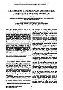
Feb 11, 2014 - Lal Hussain. University of Azad Jammu and Kashmir, Quality Enhancement Cell/ DCS &IT, Muzaffarabad, Pakistan ... 400 faces from school students in Muzaffarabad, Azad ..... the medical decision making community has an extensive .... His
dataset [26] released the same year that has 494, 414 images of 10, 575 people. The VGGFace dataset [17] released in 2015 has 2.6 million images covering 2, ...
Figure 1: The layered human model: (a) Model used to animate heads, shown as
a wireframe at ... Using Models: Thus, for both optical and video-based motion
capture, we have developed ...... puter Vision and Image Understanding 64(2), pp
.
Jan 13, 2014 - tant for applications such as tele-presence and gaming. The localized and ... implementation on a standard laptop PC. Second, it allows to ...
Jan 18, 2007 - have variable camber. Internal .... fiber composites (MFCs) from Smart Material Corp., .... Corporation, Japan) operating at 50 fields/s was.
Sagan in TAC2009: Using support vector machines in recognizing textual en- tailment and TE search pilot task. In Proc. of TAC. Clark, Peter and Phil Harrison.
Laser treatment should use small spots and just enough power to .... Cotton wool spots. A Grosso (Br J Ophthalmol, 2005) b. Cotton wool spots. âI am Lalitha Y,.
Cone. 1. 2. 0. 1 circle 1 semi-circle. Triangular Prism. 9. 5. 6. 3 x rectangle. 2 x
isosceles. Triangular Prism. 9. 5. 6. 2 x isosceles triangle. Square based pyramid.
methods used in the facial animation of synthetic actors who change their ..... research was supported by the Natural Sciences and Engineering Council of ...
May 14, 2008 - of a babyface. J Pers Soc Psychol. 48:312â323. Cunningham MR. 1986. Measuring the physical in physical attractive- ness: quasi-experiments ...
Toyota Technological Institute at Chicago .... a single bit of information is available at every pixel, mark- ... Consider a gray level image I(x, y) of a smooth Lam-.
insular cortex. Neuroimaging, as well as depth electrode recording studies, show that human insular cortex responds to disgusted faces9,10, and damage to the ...
E-mail: {stefanie.wuhrer, chang.shu, pengcheng.xi}@nrc-cnrc.gc.ca. The purpose of .... Automatic prediction of landmark positions Ben Azouz et al. [6] propose to ...
We investigate various methods for creating three-dimensional human ... Creating a human body for an actor is only the first step, his particular character ...
Sep 29, 2014 - (p,0.01) and area (p,0.01) at the posterior portion of the ventricle. Shape analysis shows that the horns exhibit a faster growth rate than the ...
integrates faces and ngerprints to make a personal identi cation. F2ID overcomes some ... Tokens may be lost, stolen, forgotten, or misplaced. PIN may be ...
tion errors occur. The corrupted observations present miss- ing data and outliers that deteriorate tracking results. We ... deform a pre-defined reference surface so as to fit data de- rived from ..... all with hard thresholding, but Eq. 6 is substit
We use facial and body animation models, not only to represent the data, but also to guide ..... A broken link in the tracked trajectory of a marker implies the loss of its identity .... the skeleton to drive the reconstruction process, as discussed
The former works best when a body part faces two or more of the cameras but ..... the skeleton to drive the reconstruction process, as discussed below. .... Correspondences are hard to establish and can be expected to be neither precise nor ...
AbstractâMotivated by the advantages of Trace transform and discrete cosine transform (DCT), an integrated face repre- sentation is proposed. In order to ...
Dec 10, 2010 - Computing EWDM(A,B) using naive method requires O(r2c2) time , which is prohibitively computationally intensive. Performing Match(a,B) ...
Neumann (Eds.), Proceedings of the Fifth European Conference on Computer Vision, Freiburg, Germany, 1998, pp. ... witness identifications for individual faces.
Dec 10, 2010 - Algorithm. Analysis. Aditya Nigam (ICARCV 2010 'SINGAPORE) ..... David A. Forsyth and Jean Ponce, Computer Vision - A Modern. Approach ...
Recognising Human Faces Using Shape and Grey-Level ... - CiteSeerX
We describe the use of flexible models for representing the shape and grey-level appearance of human faces. These mo dels are controlled by a small number ...
Recognising Human Faces Using Shape and Grey-Level Information A. Lanitis, C.J.Taylor and T.F.Cootes Dpt. of Medical Biophysics, University of Manchester Oxford Rd, Manchester M13 9PT, UK email: [email protected]
Abstract
We describe the use of flexible models for representing the shape and grey-level appearance of human faces. These mo dels are controlled by a small number of parameters which can be used to code the overall appearance of faces for classification purposes. The model parameters control both inter-class and within-class variation. Discriminant analysis techniques are employed to enhance the effect of those affecting inter-class variation, which are useful for classification. We show that with this coding scheme, good recognition results can be obtained, even when viewpoint, illumination and facial expression are al lowed to change.
1 Introduction
Automatic face recognition by machines can form a useful com ponent of many intelligent systems. Potential applications of face recognition include automatic access control, design of sophisticated robot systems that interact with humans and in dexing of face image databases. The human visual system ex hibits remarkable accuracy in recognising faces despite con siderable variations in appearance due to changes in expression, 3D orientation, lighting conditions and hairstyles. A successful automatic face identification system should be ca pable of suppressing the effect of these factors allowing any face image to be rendered expression-free with standardised 3D orientation and lighting. In this paper we describe how appear ance variation of faces can be modelled and present results for a fully automatic face identification system which tolerates ap pearance variation. For our experiments we used a database containing face images from 30 individuals. The details of that data base are shown in table 1. A second test set containing 3 face images per person was also used. For this set, subjects were asked to disguise them selves by hiding part of their face to provide a rigourous test of the robustness of the identification system. Typical images from the data sets are shown in figure 1.
2 Background
Fig. 1: Example of images used in our experiments. Training images test images and difficult test images are shown in top, middle and bottom rows respectively. expression and 3D orientation dependent, so that explicit methods of normalisation must be employed. Pentland[ 11 ] describes how principal component analysis of the grey-levels of face images can be used to create a set of ei genfaces. Any face can be approximated for identification pur poses by a weighted sum of eigenfaces. During the eigenvalue decomposition, no shape normalization takes place and for the identification system no shape information is employed. Up to 96% correct classification were reported when this approach was tested on a data base containing images from 16 individ uals. Craw[ 7 ] describes a similar method, with the difference that for his experiments the shapes of faces were normalised in order to ensure that only grey-level variations were modelled. Faces were deformed to the mean shape and principal compo nent analysis applied to obtain shape-free eigenfaces. Using this approach test faces were retrieved correctly from a data base containing 100 images; these results relied on a user inter actively locating 59 key points on each test image. When a simi lar experiment was performed using shape information alone, the results were not as good as those obtained with eigenfaces.
Face identification techniques can be divided into two main cat egories: those employing geometrical features and those using grey-level information. Most of the systems described in the lit 3 Overview erature adopt one or other (but not both) of the two possible approaches. Techniques based on geometrical fea Our approach consists of 2 main phases: training in which flex tures[ 2 , 7 , 8 ] use a number of dimensional measurements, or ible models of facial appearance are generated, and identifica the locations of a number of control points. Based on these fea tion in which facial characteristics are located and flexible mo tures faces are identified. However, geometrical features are dels are used for classifying images. Figure 2 shows the main Conditions Training Images Test Images 30 Number of subjects(classes) 10 Training images per subject Lighting conditions fixed variable 10 Test images per subject yes yes 3D movements 23 Male subjects Expression variable variable 7 Female subjects Distance from camera variable variable Ethnic origin mixed no yes Spectacles Minimum age of subjects 17 yes yes Maximum age of subjects 45 Beards/Moustaches Time period between capturing 3 - 54 no yes Hairstyle changes training/test images weeks Background fixed variable Table 1: Details of the face data set used for our experiments
Training Images Test Image
Train a Flexible Shape Model
Train Local Grey Profile Models
Locate Facial Fea tures Automatically
Extract Profiles
Shape Parameters
Local Grey Model Parameters
Train a Shape-Free Grey-Level Model
Training phase
Deform To Mean Shape Shape-Free Grey Model Parameters
Identification phase
Classification Output Figure 2: Block diagram of the face identification system elements of our approach and indicates information flow with meters and their known distributions for each class, the new in the system. face can be assigned to one of the classes. During classification discriminant analysis techniques are employed in order to en 3.1 Training sure that appearance parameters responsible for within-class are suppressed in favour of those controlling interWe have previously developed flexible models[ 4 , 5 ] in an at variation, tempt to model the appearance of variable objects. During class variation. training the main modes of variation among a set of training 4 Flexible Models examples, are established. Usually a small number of indepen Flexible models[ 4 , 5 ] are generated from training examples. dent modes of variation are enough to explain most of the vari Each training example(X ) is represented by a number of vari Á ability within a training set. Any training example can be ap ables . proximated by a weighted sum of the main modes of variation ÀÏÎ from the mean example. We refer to the weights as model para ÂÁ Ä ÀÅÃÇÉ Ê ÅÃÇË Ê ÈÈÈÊ ÅÃÇÍ Î meters. In the work reported here, the shape variation of faces was mo Where xÌ is the kth variable in the ith training example. delled using a flexible shape model. To train this model a For example, in constructing a shape model, xÌ represent the of landmark points, expressed in a standard frame number of training face outlines, represented by a number of co-ordinates landmarks, was used. Face outlines of different individuals were of reference. Equations 2 and 3 are used to calculate the aver used so that the shape variation reflected by the model ac age example(X) and the deviation of each example from the counted for both within-class and inter-class variation. Within- mean(ÁÁ). ÃÓÔ class variation is the variation observed in face images of a par ÀÖÎ Ñ ticular individual, such as changes in expression, 3D orientation Â Ä ÂÁ and lighting conditions. Inter-class variation is responsible for ÃÓÉ the differences between faces that make individuals distinctive, ÀŠÎ Ò Ä Â Á ÁÕ such as the absolute distances between features. Ideally we wish to use just inter-class information for classification so that the A principal component analysis[ 10 ] of the covariance matrix effects of expression and 3D orientation are minimised. Using of deviations is applied in order to calculate the eigenvalues and discriminant analysis techniques, we have demonstrated that eigenvectors. Each eigenvector corresponds to a specific mode this is possible[ 9 ]. variation. Any training example can be approximated using Previous authors have shown that grey-level information is ex of equation 4. tremely important in face recognition[ 3 , 7 ]. We have aug Â Ä Â Ú ÀÙÎ ÛÜ Á mented our shape model with grey-level information using two Where P is a matrix of eigenvectors different approaches. In the first we build a flexible model of ÂÂÂÂÄ is a vector of weights the appearance of shape-free faces, obtained by deforming (these are referred as Model Parameters) each face in the training set to have the same shape as the mean face. In the second approach we use a large number of local By modifying ÄÂnew instances of the model can be created; if profile models one at each point of the shape model. Each the elements of b are kept within some limits (typically 3 stan model point always corresponds to the same facial feature so dard deviations from the mean) the corresponding model in there is no need to apply a shape normalization algorithm. stances are plausible examples of the modelled object. Model Shape and grey-level models can be used together to describe parameters can be regarded as a way of monitoring whether the overall appearance of each face in terms of its model para a new example represents a legal example of the modelled ob meters; collectively we refer to the model parameters as appear ject. Equation 5 can be used to transform training examples to model parameters. ance parameters. ÀŽÎ Ü Ä ÛŸÀÂÃ Õ ÂÎ 3.2 Identification Usually the number of model parameters needed to describe Our flexible shape model can be used for locating facial char a training example adequately is much less than the original acteristics automatically[ 6 ]. When a face image is presented number of variables. to the system, an instance of the shape model is overlaid on the The same method can be used to train both shape and greyimage. Forces are applied to model points, in an iterative level models; for shape models the variables are point co-ordi scheme so as to move and deform the model, until it fits to the nates and for grey-level models, the variables are based on shape of the face presented. Based on the flexible shape model grey-level intensities. the resulting model points are transformed into shape model parameters. Grey-level information at each model point is col 5 Building a Flexible Shape Model lected and transformed to local grey-level model parameters. We have built a flexible face shape model using 152 points Then the face is deformed to the mean shape and the grey-level which were planted by hand on 160 training examples (8 appearance is transformed into the parameters of the shape- examples from 20 individuals from the data set). Typical train free grey-level model. Based on the set of appearance para ing examples and the locations of the model points are shown
in figures 3 and 4 respectively. Sixteen model parameters are needed to describe 95% of the variation within the training set. The effect of the 4 most important modes of variation on the model is shown in figure 5. Model parameters of the shape model are used as shape classification variables. However, fig ure 5 shows that some of the most significant modes of variation account only for within-class variation. For example the first 3 modes just change the 3D orientation of the model. A way of isolating parameters responsible for inter-class variation must be employed so that classification based on shape parameters is expression and 3D orientation independent.
image are moved to overlap a set of target landmarks in such a way that changes in the grey-level environment around the landmarks are kept to minimum. Fourteen landmarks were used for deforming face images. The position of these land marks on a face outline and on the average shape face outline are shown in figure 6. All landmarks are part of the shape model, implying that once the shape model has been fitted all landmarks are located automatically. In figure 7 an example of of a face image before and after deformation is shown.
Fig 6: The landmarks used for deforming face images
Fig 3: Typical training shapes
Fig 4: Model points located 1st mode 2nd mode 3rd mode 4th mode
-2sd mean +2sd Fig 5: The main modes of shape variation
Fig 7: Example of a face image (left) , the deformed image (middle) and the grey patch extracted (right). ÎÏ Ñ!"ÔÑÙ#Ô$Ú&#ÔÑ’ÕÔ*/8Ô:Ô#Ñ;Ò. For example there are modes that control the lighting conditions (1st mode), the addition of beards and moustaches (2nd mode) and the change in expression (3rd mode). Both inter-class and within-class variation are mo delled? discriminant analysis techniques can be used to separate them. Average -3sd +3sd
6 Enhancing Inter-Class Variation
Discriminant analysis [ 10 ] addresses the problem of separat ing a number of classes, given a number of variables for the training members of each class. This is achieved by enhancing the effect of inter-class variation variables. In its simplest form discriminant analysis uses the Mahalanobis distance(Di) measure, as shown in equation 6. ÄËÇ À2Á Â ÄÀ Å ÀÃÇÉ Ê-1É ÄÀ Å ÀÃÇ Where È is a multivariate observation Èi is the centroid of a multivariate distribution for a particular class Í is the covariance matrix for all classes A given multivariate observation is assigned to the class that minimises the Mahalanobis distance between the observation and the centroid of that class. Since Mahalanobis distance uses covariance information, it has the ability to suppress the effect of parameters responsible for within-class variation. 7 Building a Shape-free Face Model
ÎÏÌÑÓÔÖÒÕŠÚÛÜÑÙŸŽÔÑ ŠŸÜÔ Deformation of face images to the mean shape must be done in such a way that changes to grey-level intensities are kept to a minimum. For this purpose we have used a technique devel oped by Bookstein[ 1 ], based on thin plate splines. This allows an image to be deformed so that landmarks on the original
1st mode 2nd mode 3rd mode Fig 8: The main modes of grey-level variation 8 Building Local Grey Models
Local grey-level profile models can be used to model the greylevel appearance of faces, in the vicinity of each model point. During training, model points were overlaid on the correspon ding training images and grey-level profiles in a direction per pendicular to the boundary, extracted, as shown in figure 9. For each model point there were 160 training examples. The profile length was set to 10 pixels. Flexible profile models at each point were built using the method described in section 4. Most of
deform the shape model so that points overlap with suggested points. However in many cases the new set of preferred points may not correspond to a plausible shape representing a human face. Vector ÁÂ is converted to model parameters; if any of these parameters are outside the acceptable limits, they are forced to take the closest acceptable value. The new shape of the model is calculated by using the modified shape parameters and equa tion 4. The search method is described in more detail in [ 6 ]. This procedure ensures that model points are allowed to move only if the global constraints characterizing the shape of human faces are not violated. Even if part of a face is occluded the evidence from the rest of the model would be enough for locating all facial characteristics. Example of the original place ment and the final fitting of the model are shown in figure 11. Å
Extracted profile at the dotted line Fig. 9: Extraction of a grey profile at a model point these models need 4 model parameters to explain 95% of the variation.
9 Locating Facial Characteristics
The shape model described above can be used as an Active Shape Model[ 6 ] to fit to new faces in an iterative local optimiz ation scheme. The face model is placed on the image and is al lowed to interact dynamically until it fits to the shape of the face presented. During each iteration two main operations take place: the definition of a new suggested position for each model point and the deformation of the model in order to move as close as possible to the new preferred positions. A brief dis cussion of these operations follows.
Original placement
9.1 Definition of Suggested Positions
At each model point a profile perpendicular to the boundary is extracted and a new preferred position for that point is esti mated along the profile. For this purpose grey-level modelling techniques were employed. During training model points were overlaid on training examples; the expected grey-level profile for each model point was established. The new preferred posi tion for each point along the extracted profile is the one that looks most similar to the expected grey-level environment for that point. This procedure for a specific point is shown in figure 10. In figure 10 the new suggested position for point A is A , Expected profile Extracted profile for point A ’
A A Fig. 10: Defining the new preferred position for a model point since the grey-level profile at point A is most similar to the ex pected profile for point A. The result of this procedure is to give a new set of points (ÁÂ) containing the new preferred positions for each point. ’
’
9.2 Deforming the Shape Model
The key point of the method is that model points do not move individually to the new suggested positions. In the first place ro tation, scaling and translation of the model takes place in an at tempt to minimise the overall distance between the model points and the suggested new positions. The next step is to Shape extracted
Final fitting Fig. 11: Example of model fitting
10 Identifying Face Images
Automatic identification of faces can be performed using the flexible models described. When a new face image is presented to the system the flexible shape model is used for locating the facial characteristics automatically. Once the model is fitted the resulting model points are expressed in a standard frame of ref erence and then converted to model parameters using equation 5.(In this case ÁÄ and Á contain the co-ordinates of the standar dised resulting model points and of the average shape points, respectively). The resulting model parameters are the shape classification parameters. At each located model point, grey-level information from a profile perpendicular to the boundary is extracted. The profile data for each point is converted to model parameters for each individual point. Model parameters are used to perform clas sification based on the local grey-level models. Based on the shape model fit, the landmarks used for deform ing face images (see figure 6) are located. Target landmarks lie on the average shape; it is trivial to overlay the average face shape, and locate the target landmarks for the given image. Shape parameters
Extract profiles at model points Test image
Local profile model parameters
Shape model fitted Shape-free patch extracted
Shape-free model parameters
Deform to mean face Fig. 12: Graphical illustration of the identification procedure
Classification
Normal test set (200 images) Difficult test set(60 images) Classification Correct Correct class Correct Correct class Method time classifications within best 3 classifications within best 3 Shape Model 4 sec 70.0% 82.0% 46.7% 23.3% Shape-Free Grey-Model 30 sec 84.5% 93.0% 33.3% 48.3% Local Grey Profile Models 4 sec 84.0% 93.5% 40% 61.7% Shape + Shape-Free Model 30 sec 94.0% 99.0% 33.3% 58.3% 4 sec Shape + Profile models 91.5% 97% 33.3% 58.3% All 3 methods 30 sec 95.5% 99.0% 43.3% 71.6% All 3 methods* 30 sec* 92.0%* 94.0%* 48.0%* 67.0%* * Results for the 30 individual classification experiments (For these experiments there are 300 test and 90 difficult test images) Table 2: Results for the identification experiments These landmarks are used for deforming the face image to the The classification system was trained automatically to recogn mean face and the shape-free grey-level model parameters ise 10 more individuals without severe deterioration of the re are calculated; these parameters are also used for classification. sults. Classification of faces is achieved by using the whole set of ap pearance parameters, as calculated for the image presented. Ã3ÇAÌkÏÎÓÈÉÔÖÉÒÉÏÍÊ The multivariate distribution of these parameters, for each Andreas Lanitis is funded by a University of Manchester re class is established during training and the new image is as search studentship and an ORS award. We would like to thank signed to the class that minimises the Mahalanobis distance be members of the Department of Medical Bio-Physics for their tween the centroid of that class and the new set of appearance help and advice. Finally we thank all those who kindly volun parameters. Classification can be performed using all the 3 types of model parameters individually, or in combination. The teered to provide face images for our experiments. identification procedure is illustrated in figure 12. Ã4ÇRÉÕÉŠÉÏÌÉÊ To train the system to identify a new individual, a number of [ 1 ] F.L Bookstein. Principal Warps: Thin-Plate Splines and training images is needed. The shape model can be used for lo the Decomposition of Deformations. IEEE Transac cating automatically the model points on these images. Once tions on Pattern Analysis and Machine Intelligence, Vol model points are located the appearance parameters for train 11, no 6, pp 567-585, 1989. ing images can be calculated, and their distribution for that [ 2 ] R. Brunelli and T. Poggio. Face Recognition Through Geometrical Features. Procs of the 2nd European Con class established. By using this method new individuals are in ference on Computer Vision, pp 792-800, ed. G.Sandini, troduced to the system without the need of any extensive Springer Verlag, 1992. human labour. [ 3 ] R. Brunelli and T. Poggio. Face Recognition: Features versus Templates. IEEE Transactions on Pattern Analy ÃÃÇRÉÊËÈÍÊ sis and Machine Intelligence, Vol 15, no 10, pp Initially classification experiments using images from 20 indi 1042-1052, 1993. viduals from our database were performed; the results are [ 4 ] T.F. Cootes, C.J. Taylor, D.H. Cooper and J. Graham. shown in table 2. All experiments were performed using a sparc Training Models of Shape From Sets of Examples. Procs 10 workstation. The two methods involving grey-level informa of British Machine Vision Conference 1992, pp 9-18, eds. David Hogg and Roger Boyle, Springer Verlag, tion achieve much better results, than the method based on 1992. shape alone. These results agree with those reported by other researchers[ 3 , 7 ], suggesting that the grey-level appearance [ 5 ] T.F. Cootes, C.J. Taylor, A. Lanitis, D.H. Cooper and J. Graham. Building and Using Flexible Models Incorpo of faces is much more important for identification. However rating Grey-Level Information. Procs of the 4th Inter shape has an important classification role since classification national Conference on Computer Vision, pp 242-246, rates improve significantly when shape information is included. IEEE Computer Society Press, 1993. Using grey-level profile models proved to be the most insensi [ 6 ] T.F. Cootes, C.J.Taylor and A.Lanitis. Active Shape Mo tive to occlusions. Any of the combinations of the measures dels: Evaluation of a Multi-Resolution Method for Im produced very good results; for real time applications the proving Image Search. To appear in the Procs. of the method combining shape and grey-level profile information Machine Vision Conference , 1994. proved to be the best, whereas if increased classification accu [ 7 ] I.British Craw and P. Cameron. Face Recognition by Computer. racy is needed the shape-free grey-level model measure should Procs of British Machine Vision Conference 1992, pp be included. We subsequently introduced automatically 10 489-507, eds. David Hogg and Roger Boyle, Springer more individuals to the system and classification experiments Verlag, 1992. using all 30 individuals were performed; the results are also [ 8 ] A. Lanitis, C.J. Taylor and T.F. Cootes. A Generic Sys shown in table 2. tem For Classifying Variable Objects Using Flexible Template Matching. Procs. of British Machine Vision Ã2ÇCÎÏÌÈËÊÑÎÏÊ Conference 1993, vol 1, pp 329-338, ed. J. Illingworth, BMVA Press, 1993. We have presented an automatic face identification system. [ 9 ] A. Lanitis, C.J. Taylor and T.F. Cootes. An Automatic Both shape and grey-level information is incorporated into the Face Recognition System using Flexible Appearance system in such a way that the effects of variations in expression, Models. To appear in the Procs. of British Machine Vi 3D orientation and lighting conditions are minimised. By using sion Conference 1994. both grey-level and shape information we ensure that the [ 10 ] B.F.J. Manly. Multivariate Statistical Methods, a Primer. identification information available in faces is fully exploited. Chapman and Hall, 1986. The modelling techniques described in this paper can be used [ 11 ] M. Turk and A. Pentland. Eigenfaces for Recognition. for other applications, like face coding and reconstruction and Journal of Cognitive Neuroscience, Vol 3, no 1, pp 71-86, 1991. automatic interpretation of facial expressions and movements.