SS symmetry Article
Reconstructing Damaged Complex Networks Based on Neural Networks Ye Hoon Lee 1 and Insoo Sohn 2, * 1 2
*
Department of Electronic and IT Media Engineering, Seoul National University of Science and Technology, Seoul 01811, Korea;
[email protected] Division of Electronics and Electrical Engineering, Dongguk University, Seoul 04620, Korea Correspondence:
[email protected]; Tel.: +82-2-2260-8604
Received: 2 October 2017; Accepted: 9 December 2017; Published: 9 December 2017
Abstract: Despite recent progress in the study of complex systems, reconstruction of damaged networks due to random and targeted attack has not been addressed before. In this paper, we formulate the network reconstruction problem as an identification of network structure based on much reduced link information. Furthermore, a novel method based on multilayer perceptron neural network is proposed as a solution to the problem of network reconstruction. Based on simulation results, it was demonstrated that the proposed scheme achieves very high reconstruction accuracy in small-world network model and a robust performance in scale-free network model. Keywords: network reconstruction; neural networks; small world networks; scale free networks
1. Introduction Complex networks have received growing interest from various disciplines to model and study the network topology and interaction between nodes within a modeled network [1–3]. One of the important problems that are actively studied in the area of network science is the robustness of a network under random failure of nodes and intentional attack on the network. For example, it has been found that scale-free networks are more robust compared to random networks against random removal of nodes, but are more sensitive to targeted attacks [4–6]. Furthermore, many approaches have been proposed to optimize conventional networks against random failure and intentional attack compared to the conventional complex networks [7–10]. However, these approaches have been mainly concentrated on designing network topology based on various optimization techniques to minimize the damage to the network. So far, no work has been reported on techniques to repair and recover the network topology after the network has been damaged. Numerous solutions have been proposed on reconstruction of spreading networks based on spreading data [11–13], but the problem on the reconstruction of damaged networks due to random and targeted attacks has not been addressed before. Artificial neural networks (NNs) have been applied to solve various problems in complex systems due to powerful generalization abilities of NNs [14]. Some of the applications where NNs have been successfully used are radar waveform recognition [15], image recognition [16,17], indoor localization [18,19], and peak-to-average power reduction [20,21]. In this paper, we propose a novel network reconstruction method based on the NN technique. To the best of our knowledge, this work is the first attempt to recover the network topology after the network has been damaged and also the first attempt to apply NN technique for complex network optimization. We formulate the network reconstruction problem as an identification of a network structure based on a much reduced amount of link information contained in the adjacency matrix of the damaged network. The problem is especially challenging due to (1) very large number of possible network configurations 2 on the order of 2 N , where N is the number of nodes and (2) very small number of node interaction Symmetry 2017, 9, 310; doi:10.3390/sym9120310
www.mdpi.com/journal/symmetry
Symmetry 2017, 9, 310
2 of 11
Symmetry 2017, 9, 310
of 11 especially challenging due to (1) very large number of possible network configurations on the 2order of 2 N , where N is the number of nodes and (2) very small number of node interaction information due to nodedue removals. simplifyWe thesimplify problemthe byproblem the following (1) average(1) number of information to nodeWe removals. by theassumptions following assumptions average real connections of a network is much smaller than all the possible link configurations and (2) link number of real connections of a network is much smaller than all the possible link configurations information of M undamaged networks are available. on these we chose we the and (2) link information of M undamaged networks are Based available. Basedassumptions, on these assumptions, multiple-layer perceptron neural network (MLPNN), which is one of the frequently used NN chose the multiple-layer perceptron neural network (MLPNN), which is one of the frequently used techniques, as the of our We evaluate the performance of theofproposed method based NN techniques, as basis the basis of method. our method. We evaluate the performance the proposed method on simulations in two classical complex networks (1) small-world network and (2) scale-free based on simulations in two classical complex networks (1) small-world network and (2) scale-free networks,generated generatedby byWatts Wattsand andStrogatz Strogatzmodel modeland andBarabási Barabásiand andAlbert Albertmodel, model,respectively. respectively. networks, The rest rest of as as follows. Section 2 describes the small-world network model The of the thepaper paperisisorganized organized follows. Section 2 describes the small-world network and scale-free network, followed by the network damage model. In Section 3, we propose the model and scale-free network, followed by the network damage model. In Section 3, we propose the reconstruction method based on NN technique. In Section 4, we present the numerical results of the reconstruction method based on NN technique. In Section 4, we present the numerical results of the proposedmethod, method,and andconclusions conclusionsare aregiven givenSection Section5.5. proposed 2
Model 2.2.Model 2.1. 2.1.Small-World Small-WorldNetwork Network Small-world Small-world network network isis an animportant important network network model model with with low lowaverage average path pathlength lengthand andhigh high clustering clustering coefficient coefficient[22–24]. [22–24]. Small-world Small-world networks networks have have homogeneous homogeneous network network topology topology with with aa degree by by thethe Poisson distribution. A small-world network is created based degreedistribution distributionapproximated approximated Poisson distribution. A small-world network is created on a regular lattice such a ring of N nodes, where each node is connected to J nearest nodes. Next, the based on a regular lattice such a ring of N nodes, where each node is connected to J nearest nodes. links randomly to one of N nodes in the p. Theprobability rewiring process Next,are the links arerewired randomly rewired to one of Nnetwork nodes with in theprobability network with p. The isrewiring repeated for all is the nodes nfor =1 . N.nodes By controlling rewiring probability p, the networkp,will process repeated all. .the n = 1 … N.the By controlling the rewiring probability the interpolate between a regular lattice (p = 0) to a random network (p = 1). Figure 1 shows the detailed network will interpolate between a regular lattice (p = 0) to a random network (p = 1). Figure 1 shows algorithm foralgorithm small-world construction pseudocode the detailed for network small-world network in construction informat. pseudocode format.
1: Initialization: 2: Set the total number of nodes N 3: Set the rewiring probability p 4: Set the node degree K 5: end initialization 6: 7: for each node n (1, N) 8: Connect to nearest K nodes. 9: end for 10: 11: for each node n (1, N) 12: for each link k (1, K) 13: Generate a random number r (0, 1) 14: if r < p 15: Select a node randomly m (1, N) 16: Rewire to node m 17: end if 18: end for 19: end for
Figure Figure1.1.Small-world Small-worldnetwork networkalgorithm. algorithm.
2.2.Scale-Free Scale-FreeNetwork Network 2.2. Scale-freenetworks, networks,such suchas asBarabási Barabásiand andAlbert Albert(BA) (BA)network, network,are areevolving evolvingnetworks networksthat thathave have Scale-free degreedistribution distributionfollowing followingpower-law power-lawmodel model[4–6]. [4–6].Scale-free Scale-freenetworks networksconsist consistof ofaasmall smallnumber number degree ofnodes nodes with with very very high degree of connections. A of of connections connectionsand andrest restofofthe thenodes nodeswith withlow lowdegree degree connections. number of of m m00 nodes. nodes. Next, Next, aa new newnode nodeisis Ascale-free scale-freenetwork networkstarts startsthe theevolution evolution process process with a small number introduced to the network and attaches to m existing nodes with high degree k. The process consisting
Symmetry 2017, 9, 310 Symmetry 2017, 9, 310
3 of 11 3 of 11
introduced to the network and attaches to m existing nodes with high degree k. The process consisting of new new node node introduction introduction and and preferential preferential attachment attachment isis repeated repeateduntil untilaanetwork networkwith withNN==tt++mm0 of 0 nodes has been constructed. Figure 2 shows the detailed algorithm for scale-free network nodes has been constructed. Figure 2 shows the detailed algorithm for scale-free network construction construction pseudocode format. in pseudocodeinformat.
1: Initialization: 2: Set the initial number of nodes m0 3: Set the total number of nodes N 4: Set the node degree K 5: end initialization 6: 7: for each node n (1, m0) 8: Connect to nearest K nodes. 9: end for 10: 11: for each new node 12: Calculate the maximum degree probability as follows:
(k (h)) k (h) / k (m), m
where (k(h)) is the probability of selecting node h, k(h) is the degree of node h, and k (m) is the total number of links in the network. m
13: for each link k (1, K) 14: Connect to node m with max((k(m))) 15: end for 16: end for
Figure Figure2. 2. Scale-free Scale-free network networkalgorithm. algorithm.
2.3. 2.3. Network Network Damage Damage Model Model We Wesimulate simulatethe thedamage damageprocess processon on complex complex networks networks by by considering considering the the random random attack attack model. model. In In the the random random attack attack model, model, nodes nodes are are randomly randomly selected selected and and removed. removed. Note Note that that when when aa node node is is removed, all the links connected to that node are also removed [25]. To evaluate the performance of the removed, all the links connected to that node are also removed [25]. To evaluate the performance of proposed reconstruction method, the difference in the number of links of between the original the proposed reconstruction method, the difference in the number links between thenetwork original and the reconstructed network isnetwork used and represented as probability of reconstruction error, PRE ,error, that network and the reconstructed is used and represented as probability of reconstruction is defined as follows: PRE, that is defined as follows: NL,di f f PRE = , (1) NNLL,diff PRE , (1) where NL is the total number of existing links in the N Lcomplex network that were damaged due to random attack and NL,diff is the total number of links in the reconstructed network that are different where L is the total number of existing links in the complex network that were damaged due to from theNlinks in the original network before any node removal. For example, let us assume that the randomofattack is the thenode total pair number links in thenetwork reconstructed that number nodesand N =N4L,diff and set inofthe original is equalnetwork to Eo = {(1, 2),are (1, different 4), (2, 3), from the links in the original network before any node removal. For example, let us assume that =the (3, 4)}. If the reconstructed network has node pair set as Er = {(1, 2), (1, 3), (1, 4), (2, 3)}, then NL,diff 2 number of nodes N = 4 and the node pair set in the original network is equal to E o = {(1, 2), (1, 4), (2, and NL = 4, giving us PRE = 0.5. Note that the estimated links in the reconstructed network that were 3), (3, 4)}. original If the reconstructed node that pairwere set asnot Er =reproduced, {(1, 2), (1, 3),are (1,all 4),counted (2, 3)}, then NL,diff = not in the network, in network additionshas to links as errors. 2 and NL = 4, giving us PRE = 0.5. Note that the estimated links in the reconstructed network that were 3. Reconstruction not in the original Method network, in additions to links that were not reproduced, are all counted as errors. 3.1. Neural NetworkMethod Model 3. Reconstruction Neural networks are important tools that are used for system modeling with good generalization 3.1. Neural Network Modelto use MLPNN employing backpropagation based supervised learning in properties. We propose this work. A MLPNN has three types of layers: An input layer, an output layer, and multiple hidden
Symmetry 2017, 9, 310
4 of 11
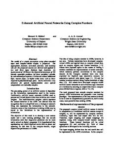
Neural are important tools that are used for system modeling with good generalization Symmetry 2017, networks 9, 310 4 of 11 properties. We propose to use MLPNN employing backpropagation based supervised learning in this work. A MLPNN has three types of layers: An input layer, an output layer, and multiple hidden layers layers in in between between the the input input and and output output layer layer as as shown shown in in Figure Figure 3. 3. The The input input layer layer receives receives input input data and is passed to the neurons or units in the hidden layer. The hidden layer units data and is passed to the neurons or units in the hidden layer. The hidden layer units are are nonlinear nonlinear activation layer. The output of of thethe jthjth unit in activation function functionof ofthe theweighted weightedsum sumofofinputs inputsfrom fromthe theprevious previous layer. The output unit the hidden layer O(j) can be represented as [26] in the hidden layer O(j) can be represented as [26] mm
j ) ∑ww((j,j,ii))O O((ii))− U (Uj ), A( jA)(= ( j ),
(2) (2)
11 , , 11+e eA−( jA) ( j)
(3) (3)
i 1
i =1
A( (Aj())j ))= O( jO) (=j ) =(
where unit, w(i, j) is weights from unit i toi to j, O(j) is where A(j) A(j)isisthe theactivation activationinput inputtotojth jthhidden hiddenlayer layer unit, w(i, j) the is the weights from unit j, O(j) the input to to unit j, U(j) is is the ) isisaanonlinear is the input unit j, U(j) thethreshold thresholdofofunit unitj, j,and and=(•() nonlinearactivation activation function function such such as as sigmoid function, as shown in Equation (3), hardlimit function, radial basis function, and triangular sigmoid function, as shown in Equation (3), hardlimit function, radial basis function, and triangular function. Thenumber numberofofunits unitsinin the output layer is equal to the dimension of desired the desired output function. The the output layer is equal to the dimension of the output data data format. The weights the network connections are adjusted using training input and format. The weights on theon network connections are adjusted using training input data anddata desired desired output data until the mean square error (MSE) between them are minimized. To implement the output data until the mean square error (MSE) between them are minimized. To implement the MPLNN, the feedforwardnet function provided by the MATLAB Neural Network Toolbox was utilized. MPLNN, the feedforwardnet function provided by the MATLAB Neural Network Toolbox was utilized. Additionally, Additionally,the theMPLNN MPLNNweights weightswere weretrained trainedusing usingthe theLevenberg-Marguardt Levenberg-Marguardtalgorithm algorithm[27]. [27].
X1 Y
X2
Input layer
Hidden layer
Output layer
Figure 3. 3. Multiple-layer neural network network (MLPNN) (MLPNN) model. model. Figure Multiple-layer perceptron perceptron neural
3.2. Neural Network Based Method 3.2. Neural Network Based Method To reconstruct the network topology of a damaged complex network due to random attack, we To reconstruct the network topology of a damaged complex network due to random attack, we apply MLPNN as a solution to solve the complex network reconstruction problem. One of the key apply MLPNN as a solution to solve the complex network reconstruction problem. One of the key design issues in MLPNN is the training process of weights on the network connections such that the design issues in MLPNN is the training process of weights on the network connections such that the MLPNN is successfully configured to reconstruct damaged networks. Usually, a complex network MLPNN is successfully configured to reconstruct damaged networks. Usually, a complex network topology is represented by an adjacency matrix describing interactions of all the nodes in the network. topology is represented by an adjacency matrix describing interactions of all the nodes in the network. However, an adjacency matrix is inappropriate as training input data for MLPNN training process However, an adjacency matrix is inappropriate as training input data for MLPNN training process due due to its complexity. Thus, we define a link list (LL) that contains binary elements representing to its complexity. Thus, we define a link list (LL) that contains binary representing existence ! elements N , where N is the number of existence of node pairs among all possible combination of node pairs N 2 N is the number of nodes of node pairs among all possible combination of node pairs , where 2 nodes in the network. For example, for a network with N = 4, possible node pair set is equal to, E = in For(2, example, network with Nto= be 4, possible node pair set isnodes equaland to, Efour = {(1, 2), {(1,the 2),network. (1, 3), (1, 4), 3), (2, 4),for (3,a4)}. If a network reconstructed has four links (1, 3), (1, 4), (2, 3), (2, 4), (3, 4)}. If a network to be reconstructed has four nodes and four links given given by E = {(1, 2), (1, 4), (2, 3), (3, 4)}, then LL = [1 0 1 1 0 1], where 1 s represents the existence of the by E =specific {(1, 2), (1, 4), (2, 3), (3,six 4)},possible then LL = [1 0 1To1 0obtain 1], where s represents existence of the four four links among ones. the 1training inputthe data, M networks are specific links among six possible ones. To obtain the training input data, M networks are damaged by damaged by randomly removing f percent of N nodes in a network. As shown in Figure 4, the randomly removing f percent of N nodes in a network. As shown in Figure 4, the proposed method
Symmetry 2017, 9, 310
5 of 11
Symmetry 2017, 9, 310
5 of 11
consists of the following modules: Adjacency matrix of damaged network input module,5adjacency Symmetry 2017, 9, 310 of 11 matrixproposed to link list transformation module, MLPNN module, andmatrix network index tonetwork adjacency method consists of the following modules: Adjacency of damaged inputmatrix proposedadjacency method consists ofsecond the following modules: Adjacency matrixmodule, of network input are transformation module. In theto the adjacency matrices ofdamaged the damaged networks module, matrix link listmodule, transformation module, MLPNN and network index module, adjacency to link listmodule. transformation module,module, MLPNN module, andmatrices network index to adjacency transformation In the the MLPNN. second adjacency of the of the pre-processed intomatrix LLs matrix that can be entered into Note the that the input dimension to adjacency matrix transformation module. the second module, thethe adjacency matrices of the of the damaged networks pre-processed into LLsInthat can be entered into MLPNN. Note that MLPNN is equal to the are dimension of the training input data format. Thus, input dimension damaged networks are ! pre-processed into LLs that can be entered into the MLPNN. Note that the input dimension of the N MLPNN is equal to the dimension of the training input data format. Thus, dimension of the theMLPNN MLPNN equal of thewhich training input data format. Thus, N . dimension MLPNN is dimension equal to of . As for the desired output isdata, the output MLPNN input isisequal toto the As for thedata, desired output which is of thethe output 2 MLPNN is equal to 2N . As for the desired output data, which is the output input dimension of the module, binary sequence numbers are usednumbers to 2represent the indices of the complex networks of the MLPNN module, binary sequence are used to represent theoriginal indices of the original of the MLPNN module, binary sequence numbers are usedofto represent theon indices of the original that have been damaged. number of MLPNN output will depend the of the training complex networks that The have been damaged. The number MLPNN output will number depend on complex networks that have been damaged. The number of MLPNN output will depend on the number of training networks used to train the MLPNN. For example, eight binary outputs will be networks used to train the MLPNN. For example, eight binary outputs will be sufficient to represent number of training networks used to train the MLPNN. For example, eight binary outputs will be sufficient to represent 256 complex networks. Based on the training input data and desired output 256 complex networks. Based on the training input data and desired output data, representing network sufficient to represent 256 complex networks. Based on the training the input data andMLPNN desired is output data, representing network topology of different complex networks, goal of the to be topology of different complex networks, the goal of the MLPNN is to be able to identify, reconstruct, data,to representing network topology of different networks,ofthe of thenetwork, MLPNN is to be able identify, reconstruct, and produce node complex pair information thegoal original among and produce pair information the original network, amongofnumerous networks used to train able to node identify, reconstruct, andof produce pair information the original network, among numerous networks used to train the neuralnode network. The detailed training algorithm of MLPNN is the neural network. The detailed training algorithm of MLPNN is described in Figure 5. numerousin networks described Figure 5.used to train the neural network. The detailed training algorithm of MLPNN is described in Figure 5. adjacency matrix of matrix adjacency damagedofnetwork
damaged network
adjacency matrix to matrix adjacency linktolist
MLPNN MLPNN
link list desired network index (in training mode) desired network index
estimated network index estimated network index
(in training mode)
adjacency matrix to matrix adjacency linktolist
network index to index network adjacency to matrix
link list
adjacency matrix
Figure 4. MLPNN based reconstruction method.
Figure 4. MLPNN based reconstruction method. Figure 4. MLPNN based reconstruction method. 1: Initialization: 2: Generate a set of M complex networks. 1: Initialization: 3: Set number of hidden layers. networks. 2: Generate a set of M complex 4: Set number of neurons in each hidden layers. 3: hidden layers. 5: Define activation function in hidden 4: Set number of neurons in each hiddenlayers. layers. 6: Set number of training iteration Iteration Num 5: Define activation function in hidden layers. 7: 6: end Initialization Set number of training iteration Iteration Num 8: 7: end Initialization 9: 8: for i = 1 : Iteration Num 10: select 9: for i =Randomly 1 : Iteration Numa complex networks m (1, M). 11: Apply random attack procedure to the m complex network m. 10: Randomly select a complex networks (1, M). 12: Obtain adjacency matrix for the damaged complex networks 11: Apply random attack procedure to the complex network m. m. 13: Transform adjacency matrix intodamaged LL. 12: Obtain adjacency matrix for the complex networks m. 14: InputTrainSeq = LL(m) 13: Transform adjacency matrix into LL. 15: DesOutputTrainSeq = dec2bin(m). 14: InputTrainSeq = LL(m) 16: 15: end for DesOutputTrainSeq = dec2bin(m). 17: 16: end for 18: 17: while estimation error > threshold do 19: for i = 1 : Iteration Num do 18: while estimation error > threshold 20: (InputTrainSeq) = MLPNN_OUT. 19: for i = 1MLPNN : Iteration Num 21: Mean Squrare Error (MLPNN_OUT, DesOutputTrainSeq). 20: MLPNN (InputTrainSeq) = MLPNN_OUT. 22: Update weightsError w in each layer using LMS algorithm. 21: Mean Squrare (MLPNN_OUT, DesOutputTrainSeq). 23: end forUpdate weights w in each layer using LMS algorithm. 22: 24: 23: end while end for 24: end while Figure 5. MLPNN training algorithm. Figure MLPNN training training algorithm. Figure 5.5.MLPNN algorithm.
Symmetry 2017, 9, 310
6 of 11
4. Performance Evaluations 4.1. Simulation Environment We study and evaluate the proposed reconstruction method based on the probability of Symmetry 2017, 9, 310 6 of 11 reconstruction error PRE described in Section 2. For the network damage model, we assume random attack process, where nodes are randomly removed with attached links. The MLPNN used in our 4. Performance Evaluations method has two hidden layers with 64 neurons in the first layer and four neurons in the second layer. 4.1. Simulation Environment The nonlinear activation function in the hidden layer is chosen to be triangular activation function. The numberWe of inputs to the MLPNN dependsreconstruction on the number of nodes thethe network. To of train and study and evaluate the proposed method basedinon probability error PRE described in Section theN network damage assumeofrandom test the reconstruction MLPNN, using complex networks with2.NFor = 10, = 30, and N = model, 50, thewe number inputs are set process, where nodes are randomly removed withwhich attached The and MLPNN used in our equal toattack the possible number of node pair combinations, arelinks. 45, 435, 1225, respectively. As method has two hidden layers with 64 neurons in the first layer and four neurons in the second layer. for the number of outputs, eight are chosen to represent maximum number of 256 complex networks. The nonlinear activation function in the hidden layer is chosen to be triangular activation function. The training input and output data patterns are randomly chosen from LL of M damaged complex The number of inputs to the MLPNN depends on the number of nodes in the network. To train and networks with differentusing percentage of failedwith nodes of=total NN nodes andnumber corresponding indices of test the MLPNN, complexfnetworks N = out 10, N 30, and = 50, the of inputs are the complex networks. set equal to the possible number of node pair combinations, which are 45, 435, and 1225, respectively. As for the number of outputs, eight are chosen to represent maximum number of 256 complex networks. Network The training input and output data patterns are randomly chosen from LL of M damaged 4.2. Small-World complex networks with different percentage f of failed nodes out of total N nodes and corresponding
To indices evaluate thecomplex performance of the proposed method in small-world network model, the network of the networks. is implemented based on the algorithm described in Figure 1. Figure 6 and Table 1 shows the 4.2. Small-World Network reconstruction error probability as a function of percentage of random node failure f. Furthermore, we study the influence of the of node the network with To evaluate the number performance of theon proposed methodreconstruction in small-world performance network model, the N = 10, based on the K algorithm described in Figure shows N = 30,network and N is= implemented 50. The initial degree of the network is Figure set to 1.two and6 and the Table links 1are randomly reconstruction error a function of percentage of randomin node f. Furthermore, rewiredthe with probability p =probability 0.15. Oneascan see that with the increase thefailure number of node failures, we study the influence of the number of node on the network reconstruction performance with N = the reconstruction performance deteriorates for all different N, but for f = 0.1, PRE is less than 0.35 and 10, N = 30, and N = 50. The initial degree K of the network is set to two and the links are randomly for f = 0.5, PRE with is less than 0.5. In another words, the proposed method can reconstruct almost close rewired probability p = 0.15. One can see that with the increase in the number of node failures, to 70% of the network fordeteriorates 10% nodeforfailures andN,more than 60% thethan network topology the reconstruction topology performance all different but for f = 0.1, PREof is less 0.35 and for 50%for node failures. Note lower reconstruction error probability is observed for larger f = 0.5, PRE is less thanthat 0.5. In another words, the proposed method can reconstruct almost close tonumber 70%The of the network for 10% and more than 60% ofof theinput network topology of nodes. reason fortopology this results is node due failures to the higher dimension data to thefor MLPNN, 50% node failures. Note that lower reconstruction error probability is observed for larger number of e.g., 1225 for N = 50. Furthermore, from the figure, we observe that PRE is less than what one might nodes. The reason for this results is due to the higher dimension of input data to the MLPNN, e.g., expect for the case where most of the nodes are destroyed, e.g., f = 0.7. This phenomenon is due to 1225 for N = 50. Furthermore, from the figure, we observe that PRE is less than what one might expect the large of overlap the node infLL among the M damaged networks fornumber the case where most ofinthe nodes areconnections destroyed, e.g., = 0.7. This phenomenon is due to the large due to small rewiring Tonode study how the rewiring probability affects networks the reconstruction accuracy, number probability of overlap inp.the connections in LL among the M damaged due to small rewiring probability p.with To study how the0.5, rewiring affects in theFigure reconstruction accuracy, simulations are performed p = 0.3, p= and p probability = 0.7, as shown 7 and Table 2. From the simulations performed p = 0.3, p =deterioration 0.5, and p = 0.7,in asperformance shown in Figure and Table 2. From figure, we can seeare that there is with a significant in7reconstruction accuracy the figure, we can see that there is a significant deterioration in performance in reconstruction with increase in rewiring probability p. This is because the small-world network topology becomes accuracy with increase in rewiring probability p. This is because the small-world network topology increasingly disordered with increase in rewiring probability and results in decrease in ability of the becomes increasingly disordered with increase in rewiring probability and results in decrease in proposed method reproduce thetooriginal network topology. ability of theto proposed method reproduce the original network topology. 0.5 N=10 N=30 N=50
PRE
0.4
0.3
0.2
0.1 0.0
0.1
0.2
0.3
0.4
0.5
0.6
0.7
0.8
0.9
f
Figure 6. Probability of reconstruction error for small-world networks with N = 10, N = 30, N = 50, M
Figure 6. Probability of reconstruction error for small-world networks with N = 10, N = 30, N = 50, = 10, and p = 0.15. M = 10, and p = 0.15.
Symmetry 2017, 9, 310
7 of 11
Symmetry 2017, 9, 310
7 of 11
Table 1. Probability of reconstruction error for small-world networks with N = 10, N = 30, N = 50, Table 1. Probability of reconstruction error for small-world networks with N = 10, N = 30, N = 50, M M = 10, and p = 0.15.
= 10, and p = 0.15. N/f N/f
0.1 0.1
0.307 10 10 0.307 30 0.273 30 2017, Symmetry 9,0.273 310 50 50 0.186 0.186
0.20.2
0.3 0.3
0.325 0.325 0.284 0.284 0.196 0.196
0.343 0.343 0.295 0.295 0.205 0.205
0.4 0.4 0.361 0.308 0.216 0.216
0.50.5 0.379 0.379 0.321 0.321 0.225 0.225
0.6 0.6 0.7 0.7 0.3970.397 0.4150.415 0.3350.335 0.3470.347 0.2340.234 0.2410.241
0.8 0.8 0.431 0.431 0.358 7 of0.358 11 0.246 0.246
Table 1. Probability of reconstruction error for small-world networks with N = 10, N = 30, N = 50, M
= 10, and p = 0.15. 0.1 0.307 0.273 0.186
P=0.3 P=0.5 0.3 P=0.7
0.2 0.325 0.7 0.284 0.6 0.196 0.8
PRE
N/f 10 30 50
0.9
0.5
0.4 0.361 0.308 0.216
0.343 0.295 0.205
0.5 0.379 0.321 0.225
0.6 0.397 0.335 0.234
0.7 0.415 0.347 0.241
0.8 0.431 0.358 0.246
0.9
0.4
0.8
0.3
0.7
P=0.3 P=0.5 P=0.7
0.6
PRE
0.2
0.5
0.1
0.00.4
0.1
0.2
0.3
0.4
0.5
0.6
0.7
0.8
0.9
f 0.3
Figure error with p =p 0.3, p =p0.5, p = p0.7, M 0.2 Figure 7. 7. Probability Probabilityof ofreconstruction reconstruction errorfor forsmall-world small-worldnetworks networks with = 0.3, = 0.5, = 0.7, =M10, and N = 50. 0.1 = 10, and N = 50. 0.0
0.1
0.2
0.3
0.4
0.5
0.6
0.7
0.8
0.9
f
Table 2. 2.Figure Probability of error for small-world networks with p = 0.3, p =p p0.5, pM = 0.7, = Table Probability ofreconstruction reconstruction small-world networks 0.3, = 0.5, p =M 0.7, 7. Probability of reconstructionerror error for for small-world networks with pwith = 0.3,pp = = 0.5, = 0.7, 10, and N = 50. 10, and M = 10,=and N =N 50.= 50. P/f
0.1
0.2
0.3
0.4
0.5
0.6
0.7
0.8
Table 2.0.1 Probability of0.2 reconstruction small-world networks p =0.6 0.3, p = 0.5, p0.7 = 0.7, M = P/f 0.3 0.3error for 0.356 0.4 0.5 with 0.315 0.319 0.334 0.373 0.399 0.431 0.477 0.8 10, and N = 50. 0.3 0.5 0.315 0.319 0.334 0.356 0.373 0.399 0.566 0.431 0.6160.477 0.430 0.438 0.457 0.477 0.494 0.524 P/f 0.1 0.438 0.2 0.3 0.4 0.50.494 0.6 0.5240.7 0.8 0.5 0.7 0.430 0.457 0.477 0.566 0.534 0.529 0.534 0.556 0.590 0.653 0.705 0.7700.616 0.3 0.334 0.356 0.373 0.431 0.477 0.7 0.534 0.315 0.5290.319 0.534 0.556 0.590 0.399 0.653 0.705 0.770 0.5
0.430
0.438
0.457
0.477
0.494
0.524
0.566
0.616
However, even in0.534 the case0.529 of high 0.534 rewiring0.556 probability 0.5, 50%0.705 of links0.770 can be successfully 0.7 0.590 p = 0.653 However, even in the case of3,high p =the 0.5, 50% ofof links can be M successfully estimated. In Figure 8 and Table we rewiring study theprobability influence of number networks that were However, the case of on high rewiring probability pthe = 0.5, 50% ofof links can be successfully estimated. In Figure 8even and 3, we study the influence of performance. number networks M that were used used to train and test theinTable MLPNN the reconstruction The number of nodes N is estimated. In Figure 8 and Table 3, we study the influence of the number of networks M that were to train and test the MLPNN on the reconstruction performance. The number of nodes N is assumed assumed to be 50 and the rewiring probability p is set to 0.5. It can be observed from the figure that used to train and test the MLPNN on the reconstruction performance. The number of nodes N is to be 50 theto rewiring probability p is setwith to p0.5. It can be observed the figure that there is a there isassumed aand small degradation performance increase PREfrom remains lessfigure than 0.3. be 50 and theinrewiring probability is set to 0.5.inItM, canbut, be observed from the that small degradation in performance with increase in M, but, P remains less than 0.3. REbut, PRE remains less than 0.3. there is a small degradation in performance with increase in M, 0.4 M=10 M=30 M=10 M=30 M=50
0.4
M=50
0.3
PRE
PRE
0.3
0.2
0.2
0.1 0.0
0.1 0.0
0.1
0.1
0.2
0.2
0.3
0.3
0.4
0.4
0.5 f
0.5
0.6
0.6
0.7
0.8
0.7
0.9
0.8
0.9
f Figure 8. Probability of reconstruction error for small-world networks with M = 10, M = 30, M = 50,
Figure 8. Probability of reconstruction error for small-world networks with M = 10, M = 30, M = 50, N = 50, and p = 0.15. Figure Probability N = 50, 8. and p = 0.15. of reconstruction error for small-world networks with M = 10, M = 30, M = 50,
N = 50, and p = 0.15.
Symmetry 2017, 9, 310 Symmetry 2017, 9, 310
8 of 11 8 of 11
Table 3. 3. Probability = 30, MM = 50, N Table Probability of of reconstruction reconstruction error errorfor forsmall-world small-worldnetworks networkswith withMM= =10, 10,MM = 30, = 50, =N50, and p = 0.15. = 50, and p = 0.15. M/f 10 10 30 30 50
M/f
50
0.1 0.186 0.186 0.218 0.218 0.26 0.1
0.26
0.2 0.2 0.196 0.196 0.226 0.226 0.267
0.3 0.3 0.205 0.205 0.233 0.233 0.267
0.267
0.4 0.4 0.216 0.216 0.239 0.239 0.269
0.267
0.5 0.5 0.225 0.225 0.246 0.246 0.274
0.269
0.6 0.6 0.234 0.234 0.253 0.253 0.279
0.274
0.279
0.7 0.8 0.7 0.8 0.241 0.246 0.2600.241 0.268 0.246 0.2850.260 0.293 0.268 0.285
0.293
4.3. Scale-Free Network 4.3. Scale-Free Network The proposed method is also evaluated in scale-free network model that is generated using the The proposed is also evaluated scale-free network that is generated using the algorithm describedmethod in Figure 2. Figure 9 andinTable 4 compares themodel reconstruction error probability algorithm described in Figure 2. Figure 9 and Table 4 compares the reconstruction error probability for different number of nodes N = 10, N = 30, and N = 50. The initial number of nodes m0 was set to for different of nodes N preferential = 30, and N attachment = 50. The initial number of nodes m0 that was the set two and the number node degree K =N 2= for10,the process. Figure 9 shows to two and the node degree K = 2 for the preferential attachment process. Figure 9 shows that the reconstruction accuracy in scale-free network model is significantly lower compared to the smallreconstruction in scale-free network model is significantly lower compared to the small-world world network.accuracy The reason for the poor performance is that the network topologies of M scale-free network. The reason for the poor performance is that the network topologies of M scale-free networks networks are more complex compared to the small-world network models. Furthermore, the links in are more complex compared to the small-world network models. Furthermore, the links in LL LL between the M damaged networks do not overlap as much as in the small-world network between models. theFigure M damaged do reconstruction not overlap as much as in the small-world network Inm Figure 10 In 10 andnetworks Table 5, the error probability performance with Nmodels. = 30 and 0 = 2, for and Table 5, the reconstruction error probability performance with N = 30 and m = 2, for different 0 the small-world different number of networks M = 10, M = 30, and M = 50, is shown. Compared to number ofenvironment, networks M = 10,reconstruction M = 30, and Merror = 50, is shown. Compared to the small-world network the probability values are quite high evennetwork in low environment, the reconstruction error probability values are quite high even in low percentage of percentage of node failures for M = 30 and M = 50. Due to the complex topology of the scale-free node failures for M = 30 and M = 50. Due to the complex topology of the scale-free network model, network model, increase in M affects the link estimation ability of the MLPNN. Finally, Figure 11 and increase in M affects the link estimation abilityperformance of the MLPNN. Finally, Figure 11 and Table of 6 shows Table 6 shows the reconstruction accuracy with different initial number nodesthe in reconstruction accuracy performance with different initial number of nodes in constructing scale-free constructing scale-free network model. One can observe that there is a small difference in network model. One can observe that there is a of small difference in reconstruction performance reconstruction performance for high percentage node failures, regardless of the initial numberfor of high percentage of node failures, regardless of the initial number of nodes. This is because the link nodes. This is because the link estimation difficulty is almost equal to the MLPNN, even if they have estimation difficulty is almost equal MLPNN, evenremains if they have different degree distributions, different degree distributions, when to thethe number of hubs the same in scale-free networks. when the number of hubs remains the same in scale-free networks. 0.8
0.7
0.6
PRE
0.5
0.4
0.3 N=10 N=30 N=50
0.2
0.1 0.0
0.1
0.2
0.3
0.4
0.5
0.6
0.7
0.8
0.9
f
Figure 9. networks with N =N10, N =N30, N =N50, M =M10, Figure 9. Probability Probability of ofreconstruction reconstructionerror errorfor forscale-free scale-free networks with = 10, = 30, = 50, = and m = 2. 10, and0 m0 = 2. Table 50, M M == 10, 10, Table 4. 4. Probability Probability of of reconstruction reconstructionerror errorfor forscale-free scale-freenetworks networkswith withNN==10, 10,N N== 30, 30, N N= = 50, and m m00 ==2.2. and N/f
0.1N/f
10 30 50
10 0.411 30 0.455 50 0.490
0.1 0.2 0.411 0.423 0.455 0.471 0.490 0.507
0.2 0.3 0.3 0.40.4 0.423 0.437 0.455 0.437 0.455 0.471 0.510 0.487 0.487 0.510 0.507 0.525 0.547 0.525 0.547
0.50.5 0.484 0.484 0.542 0.542 0.575 0.575
0.6 0.518 0.582 0.618
0.60.7
0.551 0.518 0.628 0.582 0.669 0.618
0.80.7 0.588 0.551 0.671 0.628 0.730 0.669
0.8 0.588 0.671 0.730
Symmetry 2017, 9, 310 Symmetry 2017, 9, 310
9 of 11 9 of 11
Symmetry 2017, 9, 310
9 of 11 0.9 0.9 0.8 0.8 0.7
PRE PRE
0.7 0.6 0.6 0.5 0.5 0.4 0.4 0.3 0.3 0.2 0.2 0.1 0.0
M=10 M=30 M=10 M=50 M=30 0.1M=500.2
0.3
0.4
0.1 0.0
0.1
0.2
0.3
0.4
f
0.5
0.6
0.7
0.8
0.9
0.5
0.6
0.7
0.8
0.9
f
Probabilityof ofreconstruction reconstructionerror errorfor forscale-free scale-free networks with = 10, =M 30,=M Figure 10. Probability networks with MM = 10, M =M30, 50,=N50, = N = 30, and m = 2. 30, and10. m0 Probability = 2.0 Figure of reconstruction error for scale-free networks with M = 10, M = 30, M = 50, N = 30, and m0 = 2. Table networks with MM = 10, M= M =M50, N =N30, Table 5. 5. Probability Probabilityof ofreconstruction reconstructionerror errorfor forscale-free scale-free networks with = 10, M30, = 30, = 50, = andand m05.= 30, mProbability 02.= 2. Table of reconstruction error for scale-free networks with M = 10, M = 30, M = 50, N = 30, and m0 = 2. 0.2 0.3 0.4 0.50.5 0.6 0.6 0.7 0.7 0.8 0.8 M/f M/f 0.10.1 0.2 0.3 0.4 10 0.455 0.471 0.487 0.510 0.542 0.582 0.628 0.671 M/f 0.1 0.2 0.3 0.4 0.5 0.6 0.7 0.8 10 0.455 0.471 0.487 0.510 0.542 0.582 0.628 0.671 30 0.643 0.652 0.669 0.685 0.702 0.717 0.730 0.738 0.455 0.471 0.487 0.510 0.542 0.582 30 10 0.643 0.652 0.669 0.685 0.702 0.717 0.6280.730 0.671 0.738 0.708 0.718 0.729 0.735 0.745 0.755 30 0.643 0.652 0.669 0.685 0.702 0.717 0.7300.761 0.766 0.738 0.766 50 50 0.708 0.718 0.729 0.735 0.745 0.755 0.761 0.9 50 0.708 0.718 0.729 0.735 0.745 0.755 0.761 0.766 0.9 0.8 0.8 0.7
PRE PRE
0.7 0.6 0.6 0.5 0.5 0.4 0.4 0.3
m0=2 m0=3 m0=2 m0=4 m0=3
0.3 0.2 0.2 0.1 0.0
0.1
m0=4 0.2
0.3
0.4
0.1
0.5
0.6
0.7
0.8
0.9
0.5
0.6
0.7
0.8
0.9
f 0.0
0.1
0.2
0.3
0.4 f
Figure 11. Probability of reconstruction error for scale-free networks with m0 = 2, m0 = 3, m0 = 4, N = 30, and M =11. 10.Probability Figure of reconstruction reconstructionerror errorfor forscale-free scale-freenetworks networkswith withmm 0 = 2, m0 = 3, m0 = 4, N = 30, Figure 11. Probability of 0 = 2, m0 = 3, m0 = 4, N = 30, and and M M == 10. 10. Table 6. Probability of reconstruction error for scale-free networks with m0 = 2, m0 = 3, m0 = 4, N = 30, and M6. = Probability 10. Table 6. Probability of of reconstruction reconstructionerror errorfor forscale-free scale-freenetworks networkswith withmm 2,mm00 == 3, 3, m m00 = 4, N == 30, Table 30, 0 0==2, and M == 10. 10. mo/f 0.1 0.2 0.3 0.4 0.5 0.6 0.7 0.8 0.455 0.471 0.487 0.510 0.542 0.582 0.628 0.671 m2o/f 0.1 0.2 0.3 0.4 0.5 0.6 0.7 0.8 mo /f 0.1 0.2 0.3 0.4 0.5 0.6 0.7 0.8 32 0.468 0.483 0.503 0.528 0.559 0.597 0.636 0.679 0.455 0.471 0.487 0.510 0.542 0.582 0.628 0.671 2 4 0.455 0.471 0.487 0.510 0.542 0.582 0.646 0.508 0.522 0.530 0.558 0.582 0.612 3 0.468 0.483 0.503 0.528 0.559 0.597 0.6360.628 0.689 0.679 0.671 3 0.468 0.483 0.503 0.528 0.559 0.597 0.636 0.679 4 0.508 0.522 0.530 0.558 0.582 0.612 0.646 0.689 4
0.508
0.522
0.530
0.558
0.582
0.612
0.646
0.689
5. Conclusions 5. Conclusions In this paper, we proposed a new method that efficiently reconstructs the topology of the 5. Conclusions In this paper, networks we proposed new that To efficiently the topology of the damaged complex baseda on NNmethod technique. the best reconstructs of our knowledge, our proposed In this paper, we proposed a new method that efficiently reconstructs the topology of the damaged damaged networks basedinon technique. To thethe best of our topology knowledge, our method is complex the first known attempt theNN literature to recover network after theproposed network complex networks based on NN technique. To the best of our knowledge, our proposed method is method the first known attempt in the literature to recover theNN network topology after the network has beenisdamaged and also the first known application of the technique for complex the first known attempt in the literature to recover the network topology after the network has been has been damaged and purpose also the of first known application ofathe technique network optimization. The main our work was to design NNNN solution basedfor oncomplex known damaged optimization. The main purposereconstruction. of our work was to proposed design a NN solution based on known damaged network topology for accurate The reconstruction method was evaluated network topology for accurate reconstruction. The proposed reconstruction method was evaluated
Symmetry 2017, 9, 310
10 of 11
damaged and also the first known application of the NN technique for complex network optimization. The main purpose of our work was to design a NN solution based on known damaged network topology for accurate reconstruction. The proposed reconstruction method was evaluated based on the probability of reconstruction error in small-world network and scale-free network models. From simulation results, the proposed method was able to reconstruct around 70% of the network topology for 10% node failures for small-world networks and around 50% of the network topology for 10% node failures for scale-free networks. Important topics that need to be considered in the future work is to develop a new link list that can represent both unidirectional and bidirectional link information and various performance metric needs to be developed that can be used to provide deeper understanding on the network reconstruction performance. Acknowledgments: This research was supported by Basic Science Research Program through the National Research Foundation of Korea (NRF) funded by the Ministry of Education (2017R1D1A1B03035522). Author Contributions: Insoo Sohn conceived, designed the experiments, and wrote the paper. Ye Hoon Lee analyzed data and designed the experiments. Conflicts of Interest: The authors declare no conflict of interest.
References 1. 2. 3. 4. 5. 6. 7. 8. 9. 10. 11. 12. 13. 14. 15. 16. 17. 18. 19. 20.
Wang, X.F.; Chen, G. Complex networks: Small-world, scale-free and beyond. IEEE Circuits Syst. Mag. 2003, 3, 6–20. [CrossRef] Newman, M. Networks: An Introduction; Oxford University Press: Oxford, UK, 2010. Sohn, I. Small-world and scale-free network models for IoT systems. Mob. Inf. Syst. 2017, 2017. [CrossRef] Barabási, A.; Albert, R. Emergence of scaling in random networks. Science 1999, 286, 509–512. [PubMed] Albert, R.; Barabási, A. Statistical mechanics of complex networks. Rev. Mod. Phys. 2002, 74, 47–97. [CrossRef] Barabási, A.L. Scale-free networks: A decade and beyond. Science 2009, 325, 412–413. [CrossRef] [PubMed] Crucitti, P.; Latora, V.; Marchiori, M.; Rapisarda, A. Error and attack tolerance of complex networks. Phys. A Stat. Mech. Appl. 2004, 340, 388–394. [CrossRef] Tanizawa, T.; Paul, G.; Cohen, R.; Havlin, S.; Stanley, H.E. Optimization of network robustness to waves of targeted and random attacks. Phys. Rev. E 2005, 71, 1–4. [CrossRef] [PubMed] Schneider, C.M.; Moreira, A.A.; Andrade, J.S.; Havlin, S.; Herrmann, H.J. Mitigation of malicious attacks on networks. Proc. Natl. Acad. Sci. USA 2011, 108, 3838–3841. [CrossRef] [PubMed] Ash, J.; Newth, D. Optimizing complex networks for resilience against cascading failure. Phys. A Stat. Mech. Appl. 2007, 380, 673–683. [CrossRef] Clauset, A.; Moore, C.; Newman, M.E.J. Hierarchical structure and the prediction of missing links in networks. Nature 2008, 453, 98–101. [CrossRef] [PubMed] Guimerà, R.; Sales-Pardo, M. Missing and spurious interactions and the reconstruction of complex networks. Proc. Natl. Acad. Sci. USA 2010, 106, 22073–22078. [CrossRef] [PubMed] Zeng, A. Inferring network topology via the propagation process. J. Stat. Mech. Theory Exp. 2013. [CrossRef] Haykin, S. Neural Networks: A Comprehensive Foundation; Macmillan: Basingstoke, UK, 1994. Zhang, M.; Diao, M.; Gao, L.; Liu, L. Neural networks for radar waveform recognition. Symmetry 2017, 9. [CrossRef] Lawrence, S.; Giles, C.L.; Tsoi, A.C.; Back, A.D. Face recognition: A convolutional neural-network approach. IEEE Trans. Neural Netw. 1997, 8, 98–113. [CrossRef] [PubMed] Lin, S.H.; Kung, S.Y.; Lin, L.J. Face recognition/detection by probabilistic decision-based neural network. IEEE Trans. Neural Netw. 1997, 8, 114–132. [PubMed] Fang, S.H.; Lin, T.N. Indoor location system based on discriminant-adaptive neural network in IEEE 802.11 environments. IEEE Trans. Neural Netw. 2008, 19, 1973–1978. [CrossRef] [PubMed] Sohn, I. Indoor localization based on multiple neural networks. J. Inst. Control Robot. Syst. 2015, 21, 378–384. [CrossRef] Sohn, I. A low complexity PAPR reduction scheme for OFDM systems via neural networks. IEEE Commun. Lett. 2014, 18, 225–228. [CrossRef]
Symmetry 2017, 9, 310
21. 22. 23. 24. 25. 26. 27.
11 of 11
Sohn, I.; Kim, S.C. Neural network based simplified clipping and filtering technique for PAPR reduction of OFDM signals. IEEE Commun. Lett. 2015, 19, 1438–1441. [CrossRef] Watts, D.; Strogatz, S. Collective dynamics of ‘small-world’ network. Nature 1998, 393, 440–442. [CrossRef] [PubMed] Kleinberg, J.M. Navigation in a small world. Nature 2000, 406, 845. [CrossRef] [PubMed] Newman, M.E.J. Models of the small world. J. Stat. Phys. 2000, 101, 819–841. [CrossRef] Holme, P.; Kim, B.J.; Yoon, C.N.; Han, S.K. Attack vulnerability of complex networks. Phys. Rev. E 2002, 65, 1–14. [CrossRef] [PubMed] Johnson, J.; Picton, P. How to train a neural network: An introduction to the new computational paradigm. Complexity 1996, 1, 13–28. [CrossRef] Marquardt, D.W. An algorithm for least-squares estimation of nonlinear parameters. J. Soc. Ind. Appl. Math. 1963, 11, 431–441. [CrossRef] © 2017 by the authors. Licensee MDPI, Basel, Switzerland. This article is an open access article distributed under the terms and conditions of the Creative Commons Attribution (CC BY) license (http://creativecommons.org/licenses/by/4.0/).