has long been a fundamental problem in computer vision. The reconstructed ... the past decades, obtaining high-quality dense depth data is still a challenging ...
Recovering Consistent Video Depth Maps via Bundle Optimization Guofeng Zhang1 1
Jiaya Jia2
Tien-Tsin Wong2
State Key Lab of CAD&CG, Zhejiang University {zhangguofeng, bao}@cad.zju.edu.cn
input sequence
2
Hujun Bao1
The Chinese University of Hong Kong {leojia, ttwong}@cse.cuhk.edu.hk
output video depth maps
Figure 1. High-quality depth reconstruction from the video sequence “Road” containing complex occlusions. Left: An input video sequence taken by a moving camera. Right: Video depth maps automatically computed by our method. The thin posts of the traffic sign and street lamp, as well as the road with graduate depth change, are accurately constructed in the recovered depth maps.
Abstract This paper presents a novel method for reconstructing high-quality video depth maps. A bundle optimization model is proposed to address the key issues, including image noise and occlusions, in stereo reconstruction. Our method not only uses the color constancy constraint, but also explicitly incorporates the geometric coherence constraint associating multiple frames in a video, thus can naturally maintain the temporal coherence of the recovered video depths without introducing over-smoothing artifact. To make the inference problem tractable, we introduce an iterative optimization scheme by first initializing disparity maps using segmentation prior and then refining the disparities by means of bundle optimization. Unlike previous work estimating complex visibility parameters, our approach implicitly models the probabilistic visibility in a statistical way. The effectiveness of our automatic method is demonstrated using challenging video examples.
1. Introduction Stereo reconstruction of dense depths from real images has long been a fundamental problem in computer vision. The reconstructed depths can be used by a wide spectrum of applications including 3D modeling, robot navigation, image-based rendering, and video editing. Although stereo problem [14, 8, 15, 23] has been extensively studied during the past decades, obtaining high-quality dense depth data is still a challenging problem due to many inherent difficulties, such as image noise, textureless pixels, and occlusions.
Given an input video sequence taken by a freely moving camera, we propose a novel method to automatically construct high-quality and consistent depth maps for all frames. Our main contribution is the development of a global optimization model based on multiple frames, which we called bundle optimization, to resolve most of the aforementioned difficulties in disparity estimation. Our method does not explicitly model the binary visibility (occlusion). Instead, the visibility is encoded naturally in the energy definition. Our model also does not distinguish among image noise, occlusions and estimation errors, so as to achieve a unified framework in modeling matching ambiguities. The color constancy constraint and geometric coherence constraint linking different views are combined in an energy minimization framework, reliably reducing the influence of image noise and occlusions in a statistical way. This process makes our optimization not produce over-smoothing or blending artifact. In order to deal with the disparity estimation in textureless region and alleviate the problem of segmentation especially on fine object structures, we only use the image segmentation prior in the disparity initialization. Then our iterative optimization algorithm refines the segmented disparities in a pixel-wise manner. Experiments show that this is rather effective in estimating correct disparities in textureless regions while faithfully preserving the fine structures of object silhouettes. Our method is very robust against occlusions, matching ambiguities, and noise. We have conducted experiments on a variety of challenging examples. Automatically computed depth maps contain very little noise. Clear object silhou-
ettes are also preserved. One challenging example is shown in Figure 1, in which the scene contains large textureless regions, objects with strong occlusions, road with smooth depth change, and even the thin posts of traffic sign and street lamp. Our method faithfully reconstructs all these structures and naturally preserves object silhouettes. Readers are referred to our supplementary video for inspecting the temporal consistency among the recovered depth maps1 .
2. Related Work Multi-view stereo algorithms [12, 2, 8, 23] estimate depth or disparity with the input of multiple images. Early approaches [12, 2] used local and window-based methods, and employed a local “winner-takes-all” (WTA) strategy in depth estimation at each pixel. Later on, several global methods [10, 19, 8] were proposed, which formulate the depth estimation as an energy-minimization problem, and commonly apply graph cuts or belief propagation to solve it. It is known that loopy belief propagation and multi-label graph cuts do not guarantee global optimal solutions in energy minimization, especially when the matching costs are not distinctive in textureless areas. By assuming that the neighboring pixels with similar colors have similar or continuous depth values, segmentationbased approach [20, 21, 9] can improve the depth estimation especially for large textureless regions. These methods typically model each segment as a 3D plane and estimate the plane parameters by matching small patches between neighboring viewpoints [21, 9], or using a robust fitting algorithm [20]. In [5, 1], non-fronto-parallel planes were constructed on sparse 3D points obtained by structure from motion. Recently, Zitnick and Kang [23] proposed an over-segmentation method to produce segments containing sufficient information for matching while reducing the risk of spanning a segment over multiple layers. However, even with over-segmentation or soft segmentation, the segmentation errors still inevitably affect the disparity estimation. Occlusion handling is another major issue in stereo matching. Methods in [8, 16, 18, 17] use explicit occlusion labeling in disparity estimation. Kang and Szeliski [8] proposed to combine several techniques, i.e. shiftable windows, temporal selection, and explicit occluded pixel labeling, to handle occlusions in dense multi-view stereo within a global energy minimization framework. Methods described in [16, 18, 17] explicitly incorporate the visibility variables in optimization. However, for dealing with a large set of images, a large amount of visibility variables will make the inference difficult. Traditional multi-view stereo methods compute the local depth map associated with each chosen reference frame 1 The supplementary video can be downloaded from the following site: http://www.cad.zju.edu.cn/home/gfzhang/projects/videodepth.
independently, which typically results in distracting reconstruction noise and temporally inconsistent depth recovery in a video. Kang and Szeliski [8] proposed to simultaneously optimize a set of depth maps at multiple key-frames, by adding a temporal smoothness term. This method indeed makes the disparities across frames vary smoothly. However, it is sensitive to outliers and may lead to blending artifacts around object boundaries. In our method, rather than using direct smoothing or blending of disparities, we introduce a geometry term which helps to maintain the temporal coherence by measuring the reconstruction noise and probabilistic visibility in a statistical way. This makes our disparity estimation robust against outliers and noise. As a result, the cost distribution of our data term is distinctive, making our optimization stable. Multi-view stereo methods for reconstructing 3D object models also have been widely investigated [15]. Many of them are proposed to model single object and cannot be applied to handling large-scale scenes owing to the issues of computation complexity and memory space requirement. Gargallo and Sturm [6] proposed to formulate the 3D modeling from images as a Bayesian MAP problem, using multiple depth maps. Recently, Merrell et al. [11] proposed a quick depth map fusion method to construct a consistent surface. They employed a weighted blending method based on the visibility constraint and confidences. In comparison, our method combines color constancy and geometric coherence constraints, thus can robustly estimate consistent view-dependent depth maps across video frames. In summary, many approaches have been proposed to model 3D objects and estimate depths using multiple input images. However, the issue of how to appropriately extract useful information in recovering depths from videos is still not addressed well. In this paper, we show that by appropriately maintaining the temporal coherence based on the color and geometry constraints, surprisingly consistent dense depth maps can be estimated from video sequences. The recovered consistent depth maps can also be used in other applications such as view interpolation, depth-based segmentation, and layer extraction.
3. Disparity Model Given a video sequence Iˆ with n frames, Iˆ = {It |t = 1, ..., n}, taken by a freely moving camera, our objective is ˆ = {Dt |t = 1, ..., n}. to estimate a set of disparity maps D Here, It (xt ) denotes the color (or intensity) of pixel xt in frame t. It is a 3-vector in a color image or a scalar in a grayscale image. Denoting by zxt the depth value of pixel xt in frame t, by convention, the disparity parameter Dt (xt ) (dxt for short) is defined as dxt = 1/zxt . The camera parameter set for frame t in a video sequence is denoted as Ct = {Kt , Rt , Tt }, where Kt is the intrinsic matrix, Rt is the rotation matrix, and Tt is the trans-
lation vector. The parameters for all frames can be estimated reliably by the structure from motion (SFM) techniques [7, 13, 22]. Our system employs the SFM method proposed by Zhang et al. [22]. In order to robustly estimate a set of disparity maps, we define the following energy in a video: ˆ I) ˆ = E(D;
n X
ˆ D\D ˆ t ) + Es (Dt )), (Ed (Dt ; I,
^ Xt '
^ Xt
lt ',t ( x t ' )
(1)
l t ,t ' ( x t ) x
t ' →t t
xt
xt'
t=1
ˆ where the data term Ed measures how well the disparity D ˆ and the smoothness term Es enfits the given sequence I, codes the smoothness on disparities. For each frame t, the disparity map Dt should not only satisfy the color constancy constraint, but also satisfy a geometric coherence constraint associating other frames in a video. We call our model the bundle optimization model because the disparities of different frames are explicitly correlated and optimized in an energy minimization framework.
3.1. Data Term Definition Data term definition usually plays an essential role in energy minimization. If the cost distribution of a data term is uninformative, the unreliable cost measurement makes the optimization problematic. For instance, if we define the data term as the color similarity, in textureless areas or occlusion boundaries, there must exist strong matching ambiguity. Using smoothness assumption only compromises the disparity of one pixel to its neighborhood, but does not help too much to infer the true value. Another issue of designing data term for depth estimation is occlusion handling. Visibility terms with binary values are commonly introduced in many stereo matching methods [8, 18]. Specifically, if the matching cost errors or the errors by some other inconsistency measurements of disparities are above a threshold, the pixels are labeled “occluded”. Obviously, the binary definition is not always optimal since the threshold or other parameters usually need to be tuned for various scenes and it is difficult to “softly” incorporate the visibility in energy minimization. In our data term definition, to make the cost distinctive, we simultaneously consider the statistical information from both color and geometry. Specifically, in a video sequence, if the disparity of one pixel in one frame is mistakenly estimated due to either occlusion or other factors, the projection of this pixel to other frames using the incorrect disparity has small probability simultaneously satisfying both color and geometry constraints. By using this information, our method is able to automatically and robustly detect the disparity errors so as to improve disparity estimation for pixels around object silhouettes. Considering a pixel xt in frame t, by epipolar geometry, the matching pixel in frame t0 should lie on the conjugate
x tt '→t = lt ',t ( x t ' , d x t ' ))
x t ' = lt ,t ' ( x t , d x t ) Ct '
Ct
Figure 2. Geometric coherence constraint. The conjugate pixel of xt in frame t0 is denoted as xt0 and lies in the conjugate epipolar line. Ideally, when we project xt0 from frame t0 back to t, the 0 projected pixel should satisfy xtt →t = xt . However, in disparity 0 estimation, the matching process causes errors, making xtt →t and xt be two different pixels.
epipolar line. Given the estimated camera parameters and the disparity dxt for pixel xt , we compute the conjugate pixel location in It0 by −1 h > xht0 ∼ Kt0 R> t0 Rt Kt xt + dxt Kt0 Rt0 (Tt − Tt0 ),
(2)
where superscript h denotes the vector in homogeneous coordinate. The 2D point xt0 is computed by dividing xht0 by the scaling factor. We denote the mapping pixel in frame t0 from xt as xt0 = lt,t0 (xt , dxt ). The mapping lt0 ,t is sym0 metrically defined. So we also have xtt →t = lt0 ,t (xt0 , dxt0 ). An illustration is shown in Figure 2. If there is no occlusion or matching errors, ideally, we 0 have xtt →t = xt . So we define the likelihood of disparity d for any pixel xt in It by combining two different constraints: X (3) L(xt , d) = pc (xt , d, It , It0 ) · pv (xt , d, Dt0 ), t0
where pc (xt , d, It , It0 ) measures the color similarity between pixel xt and the projected pixel lt,t0 (xt , d) in frame t0 and is defined as σc , pc (xt , d, It , It0 ) = σc + ||It (xt ) − It0 (lt,t0 (xt , d))|| where σc controls the shape of our differentiable robust function, and is set to 10 in all our experiments. ||It (xt ) − It0 (lt,t0 (xt , d))|| is the color L-2 norm. The value of pc (xt , d, It , It0 ) is in the range of (0,1]. pv (xt , d, Dt0 ) is the proposed geometric coherence term 0 measuring how close pixels xt and xtt →t are in image space, as shown in Figure 2. For ease of explanation, we first define pv (xt , d, Dt0 ) as exp(−
||xt − lt0 ,t (xt0 , Dt0 (xt0 ))||2 ), 2σd2
(4)
which is in a form of Gaussian distribution, where σd denotes the standard deviation. Both the above color and geometry constraints use the corresponding pixel information when mapping from frame t0 to frame t. But they constrain the disparity in two different ways. In the following, we briefly explain why the simple likelihood definition in (3) can be used effectively in disparity estimation without explicitly modeling occlusion. The above likelihood definition requires the correct disparity to be supported by two constraints simultaneously, i.e. high color similarity as well as high geometric coherence. An erroneously estimated disparity value for one pixel seldom satisfies both color and geometry constraints, generally making pc (xt , d, It , It0 ) · pv (xt , d, Dt0 ) small. So, from a statistics perspective, considering the 0 mappings P from all other frames t to t, incorrect disparity makes pc (·) · pv (·) output very small value. In contrast, a correct d makes pc (xt , d, It , It0 )·pv (xt , d, Dt0 ) output comparably large values for all unoccluded pixels. This results in a highly non-uniform cost distribution for each pixel favoring true disparity values. In [8], an extra temporal smoothness term was introduced outside the data term definition, which functions similarly to the spatial smoothness constraint. It compromises the disparities temporally, but does not help too much to infer true disparity values. Equation (4) introduces a simple geometric coherence constraint formulation. In our method, due to the errors or noise inevitably introduced in various parameter estimation and optimization processes, the disparity estimation D(x) may deviate from its true position. It is reasonable to assume that a better disparity value of x can be found in the near neighbors of x. So we modify (4) to pv (xt , d, Dt0 ) =
max w
x 0 ∈W (xt0 ) t
exp(−
||xt − lt0 ,t (xt0 , dxw )||2 t0 2σd2
),
(5)
where W (xt0 ) denotes a window centered at xt0 . Its size is set to 5 × 5 in our experiments. The value of standard deviation σd is set to 3. The window search in (5) empirically makes the energy decrease faster and our optimization process be more stable. Using the likelihood definition in (3), our data term Ed is defined as ˆ D\D ˆ t) = Ed (Dt ; I,
X
1 − u(xt ) · L(xt , Dt (xt )) (6)
xt
for cost minimization. u(xt ) = 1/ max L(xt , Dt (xt )), is Dt (xt )
a normalization factor. Our data cost performs better than that using color constancy constraint alone, making it possible to reliably compute disparities along object silhouettes and handle matching errors and occlusions.
3.2. Smoothness Term The smoothness term is simply defined as Es (Dt ) =
X
X
λ(xt , yt ) · ρ(Dt (xt ), Dt (yt )),
(7)
xt yt ∈N (xt )
where N (xt ) denotes the neighbors of pixel xt , and λ is the smoothness weight. ρ(·) is a robust function defined by ρ(Dt (xt ), Dt (yt )) = min{|Dt (xt ) − Dt (yt )|, η}, where η determines the upper limit of the cost. In order to preserve discontinuity, λ(xt , yt ) is usually defined in an anisotropic way, encouraging disparity discontinuities coincident with intensity/color change. Our adaptive smoothness weight is defined as λ(xt , yt ) = ws ·
uλ (xt ) ||It (xt ) − It (yt )|| + ε
where uλ (xt ) is a normalization factor and defined as X 1 uλ (xt ) = |N (xt )|/ . ||I (x ) − It (yt0 )|| + ε t t 0 yt ∈N (xt )
ws denotes the smoothness strength and ε controls the contrast sensitivity. Our adaptive smoothness term imposes smoothness in flat regions while preserving edges in textured regions.
4. Bundle Optimization Minimizing the energy defined in (1) is not straightforward since estimating the dense disparity maps for all video frames in one pass is computationally intractable. In this section, we introduce an iterative optimization algorithm and associate each video frame to its neighborhood by multi-view geometry. The corresponding disparity maps are improved by maintaining necessary color and geometry constraints. Iterative optimization generally requires a good starting point to make the optimization process robust and converge rapidly. In our disparity estimation problem, to better handle textureless regions, we incorporate the segmentation information into the initialization. It is widely known that segmentation is a double-edged sword. On one hand, segmentation-based approaches usually improve the quality of disparity result in large textureless regions. On the other hand, they inevitably introduce errors in textured regions and do not handle well the situation that similar-color pixels are with different disparity values, even using oversegmentation. Our iterative optimization takes the advantage of segmentation by incorporating it into our initialization while limiting its problems by performing pixel-wise disparity refinement in the following optimization. Table 1 gives an overview of our framework. We describe the implementation of all steps in Section 4.1 and 4.2.
1. Structure from Motion: 1.1 Recover the camera parameters. 2. Disparity Initialization: 2.1 Apply loopy belief propagation to minimize (8). 2.2 Combine image segmentation to further improve the initial disparities. 3. Bundle Optimization: 3.1 Process frames from 1 to n: For each frame t, fix disparities in other frames and refine Dt by minimizing (1). 3.2 Repeat step 3.1 for at most 2 passes. 3.3 Final accuracy refinement by nonlinear continuous optimization. Table 1. Overview of our framework.
4.1. Disparity Initialization Denoting the disparity range as [dmin , dmax ], we equally quantize the disparity into m + 1 levels where the kth level dk = (m − k)/m · dmin + k/m · dmax , k = 0, ..., m. In the beginning, the disparity maps of the whole sequence are unknown. So the energy defined in (1) cannot be directly minimized. To make the computation feasible, we separately estimate the disparity map for each frame by removing the geometric coherence constraint from the likelihood definition in (3) and modify it to X pc (xt , Dt (xt ), It , It0 ). Linit (xt , Dt (xt )) = t0
So (1) is also correspondingly modified to ˆ I) ˆ = Einit (D;
n X X
(1 − u(xt ) · Linit (xt , Dt (xt )) +
t=1 xt
X
λ(xt , yt ) · ρ(Dt (xt ), Dt (yt ))), (8)
yt ∈N (xt )
where the normalization factor u(xt ) is defined as u(xt ) = 1/ max Linit (xt , dk ). Using Einit , the disparity maps of k
different frames are not directly correlated by a geometric coherence constraint. So we can optimize Dt for each frame t separately. Taking into account the possible occlusions, it is better to only select the frames where the pixels are visible rather than summing the matching errors over all frames. We employ the temporal selection method proposed in [8] to improve the matching correctness. Then for each frame t, we use loopy belief propagation [4] to estimate Dt by minimizing (8). Figure 3(b) shows one frame result obtained in this step (i.e., step 2.1 in Table 1). The estimated disparities are not correct for many pixels, especially in textureless regions. We then incorporate the segmentation information into our initialization to handle textureless regions. The seg-
ments of each frame are obtained by a mean-shift color segmentation [3]. Similar to the non-fronto-parallal techniques [20, 18], we model each segment in disparity as a 3D plane and define plane parameters [ai , bi , ci ] for each segment si . Then, for each pixel x = [x, y] ∈ si , the corresponding disparity is given by dx = ai x + bi y + ci . Taking dx into (8), Einit is formulated as a nonlinear continuous function w.r.t. the variables ai , bi , ci , i = 1, 2, .... The partial derivatives over ai , bi , ci must be computed when applying a nonlinear continuous optimization to estimating all 3D plane parameters. Since Linit (x, dx ) does not directly depend on the plane parameters, we apply the following chain rule: ∂Linit (x, dx ) ∂dx ∂Linit (x, dx ) ∂Linit (x, dx ) = · =x . ∂ai ∂dx ∂ai ∂dx Similarly,
∂Linit (x,dx ) ∂bi
∂Linit (x,dx ) . ∂dx
(x,dx ) = y ∂Linit and ∂dx
∂Linit (x,dx ) ∂ci
=
∂Linit (x,dx ) ∂dx
In these equations, is firstly computed on quantized disparity levels by estimating the gradients: Linit (x, dk+1 ) − Linit (x, dk−1 ) ∂Linit (x, dx ) |d k = , ∂dx dk+1 − dk−1 where k = 0, ..., m. Then the continuous function Lcinit (x, dx ) is formed by cubic-Hermite interpolation. Finally, the continuous partial derivatives are calculated on Lcinit (x, dx ). Since dx = ai x + bi y + ci , estimating disparity variable dx is equivalent to estimating plane parameters [ai , bi , ci ]. We thus use a nonlinear continuous optimization method to estimate the plane parameters by minimizing the energy function (8). Initial 3D plane parameter values can be obtained by non-fronto-parallel planes extraction methods [20, 5, 1]. In practice, we adopt a much simpler method which can already produce satisfying initial values. Particularly, for each segment si , we fix ai = 0 and bi = 0 (i.e., assuming fronto-parallel plane), and also fix the disparity values in other segments. Then we compute a set of ci by different assignments of dk where k = 0, ..., m and select the best c∗i minimizing the energy function (8). After the above process, we further refine the initialized 3D plane parameters [0, 0, c∗i ] by minimizing energy function (8) using the Levenberg-Marquardt method. We show in Figure 3 one frame example. Figure 3(c) illustrates the incorporated segmentation during initialization. The disparity result after initialization is shown in Figure 3(d).
4.2. Iterative Optimization in a Video After incorporating segmentation in disparity initialization for individual video frames, disparity estimation is improved in textureless regions. However, there still exist errors, especially around occlusion boundaries as illustrated in Figure 3(d) and (g). Besides, since the disparity maps are
(a)
(b)
(d)
(e)
(c)
(f)
(g)
(h)
Figure 3. Bundle optimization illustration. (a) One frame from the “Road” sequence. (b) The inital result after solving (8) by belief propagation. (c) Segmentation prior incorporated into our initialization. (d) Initialization result after segmentation and plane fitting using nonlinear continuous optimization. (e) Our final disparity result after bundle optimization. (f)-(h) Magnified regions from (a), (d), and (e), showing that our bundle optimization improves disparity estimation significantly on object boundaries.
independently estimated, the temporal consistency among them is not adequately maintained. The inconsistency can be easily noticed in video sequence playback, as illustrated in our supplementary video. To address this problem, we take the geometric coherence constraint associated with multiple frames into the data term definition, and iteratively refine the results by minimizing the energy defined in (1), using loopy belief propagation. Each pass starts from frame 1. With the concern of computation complexity, in processing video frames, we refine disparity map Dt while fixing the disparities of all other frames. The data term only associates frame t with 20-30 neighboring frames. One pass completes when the disparity map of frame n is optimized. In our experiments, at most two passes are sufficient to produce temporally consistent disparity maps. After the above processes, the obtained disparities are all discrete values. So we introduce a nonlinear continuous optimization method to further refine them. The continuous data cost is computed using cubic-Hermite interpolating function, similar to that described in Section 4.1. Then we repeat above disparity estimation process: for each frame t, we fix the disparities of all other frames, and refine the disparity map Dt using a continuous steepest descent method.
5. Experimental Results To evaluate the performance of the proposed method, we have conducted experiments on several challenging sequences. In all our experiments, we set the maximal disparity level m = 100, ws = 5/(dmax − dmin ), η =
(a)
(b)
(c)
(d)
Figure 4. Disparity results on the “Flower Garden” sequence. (a)(b) 10th frame and 20th frame in the input sequence. (c)-(d) The estimated disparity maps for (a)-(b) respectively. The complete sequence is included in our supplementary video.
0.05(dmax − dmin ), and ε = 20. Table 2 lists the statistics of the tested sequences. Our bundle optimization converges rapidly, where two passes are sufficient for all examples. The processing time is a few minutes for each video frame. The computation is mostly spent on the data cost computation considering all pixels in multiple frames. Figure 3 shows one example. The “Road” sequence contains large textureless areas with complex occlusions, which makes stereo reconstruction difficult. During our initialization, by solving the energy function (8), the estimated
(a)
(b)
(c)
(d)
(e)
(f)
(g)
(h)
(i)
Figure 5. Disparity results on the “Angkor Wat” sequence. (a)-(c) The 70 frame, 80 frame, and 90 frame of the input sequence. (d)-(f) The estimated disparity maps for (a)-(c) respectively. For illustration of correctness, we warped one frame to another by the estimated disparities. (g) Warping 70th frame to 90th frame. (h) Warping 80th frame to 90th frame. (i) From left to right: magnified regions of (g), (h), and (c) respectively. The purely black pixels are the missing pixels in the 3D warping. Our warping result, even near discontinuous object boundaries, is natural, which indicates that our estimated disparities are accurate. The complete sequence is included in our supplementary video. th
sequence frames resolution
Road 141 960×540
Angkor Wat 129 576×352
Garden 150 352×240
Temple 121 576×352
Table 2. The information of the tested sequences contained in the supplementary video and shown in this paper.
disparity map is shown in Figure 3(b). By incorporating segmentation prior, the disparities are refined as shown in Figure 3(d). After our bundle optimization, the temporal consistency is preserved in the recovered video disparity maps. The reconstruction errors especially around occlusion boundaries are reduced. The result is shown in Figure 3(e) and the comparison is given in (g) and (h). The “Angkor Wat” sequence example is shown in Figure 5. This sequence also contains complex occlusions and large textureless areas, such as the sky and the yard. As shown in our results, our approach produces accurate and
th
th
consistent disparities even near discontinuous object boundaries. This is demonstrated by projecting one frame to others using 3D warping, and comparing the boundary structures, as illustrated in (g), (h), and (i). Figure 4 shows two frames extracted from the “Flower Garden” sequence. The disparity reconstruction results are also natural and consistent, especially along the tree trunk. The disparities surrounding the branches inherently have ambiguity regarding almost constant-color background sky. These regions can be interpreted as either in the background sky, or in a foreground layer with unknown disparities.
6. Conclusions In this paper, we have proposed a novel method for constructing high-quality depth maps from a video. Our method advances the stereo reconstruction in a few ways. First, based on the geometry constraint, we model the prob-
abilistic visibility and reconstruction noise using statistical information simultaneously considering multiple frames. This model handles occlusions as well as matching errors in a unified framework. Second, by combining the color constancy constraint and geometric coherence constraint, our data cost is well-posed even in textureless areas and occlusion boundaries. This makes a standard discrete optimization solver, such as BP, converges quickly within a small number of iterations. Third, we do not directly use segmentation in handling textureless regions, but rather employ it in the initialization. Therefore, our method is capable of faithfully reconstructing fine structures. As discussed in [15], reconstructing complete 3D models from real images is still a challenging problem. Many of the methods aim to model a single object and they have inherent difficulties to model complex outdoor scenes. In comparison, our method can automatically estimate temporally consistent view-dependent depth maps. We believe this work will not only benefit the 3D modeling, but also easily find applications in video processing, rendering, and understanding.
Acknowledgements This work is supported by NSF of China (No.60633070), 973 program of China (No.2002CB312104), and the Research Grants Council of the Hong Kong Special Administrative Region, under RGC Earmarked Grants (Project No. CUHK417107 and 412307).
References [1] P. Bhat, C. L. Zitnick, N. Snavely, A. Agarwala, M. Agrawala, B. Curless, M. Cohen, and S. B. Kang. Using photographs to enhance videos of a static scene. In J. Kautz and S. Pattanaik, editors, Rendering Techniques 2007 (Proceedings Eurographics Symposium on Rendering), pages 327–338. Eurographics, June 2007. 2, 5 [2] R. T. Collins. A space-sweep approach to true multi-image matching. In CVPR, pages 358–363, 1996. 2 [3] D. Comaniciu and P. Meer. Mean shift: A robust approach toward feature space analysis. IEEE Trans. Pattern Anal. Mach. Intell., 24(5):603–619, 2002. 5 [4] P. F. Felzenszwalb and D. P. Huttenlocher. Efficient belief propagation for early vision. International Journal of Computer Vision, 70(1):41–54, 2006. 5 [5] D. Gallup, J.-M. Frahm, P. Mordohai, Q. Yang, and M. Pollefeys. Real-time plane-sweeping stereo with multiple sweeping directions. In CVPR, 2007. 2, 5 [6] P. Gargallo and P. F. Sturm. Bayesian 3D modeling from images using multiple depth maps. In CVPR (2), pages 885– 891, 2005. 2 [7] R. Hartley and A. Zisserman. Multiple View Geometry in Computer Vision. Cambridge University Press, 2000. 3
[8] S. B. Kang and R. Szeliski. Extracting view-dependent depth maps from a collection of images. International Journal of Computer Vision, 58(2):139–163, 2004. 1, 2, 3, 4, 5 [9] A. Klaus, M. Sormann, and K. F. Karner. Segment-based stereo matching using belief propagation and a self-adapting dissimilarity measure. In ICPR (3), pages 15–18, 2006. 2 [10] V. Kolmogorov and R. Zabih. Computing visual correspondence with occlusions via graph cuts. In ICCV, pages 508– 515, 2001. 2 [11] P. Merrell, A. Akbarzadeh, L. Wang, P. Mordohai, J.-M. Frahm, R. Yang, D. Nist´er, and M. Pollefeys. Real-time visibility-based fusion of depth maps. In ICCV, 2007. 2 [12] M. Okutomi and T. Kanade. A multiple-baseline stereo. IEEE Trans. Pattern Anal. Mach. Intell., 15(4):353–363, 1993. 2 [13] M. Pollefeys, L. J. V. Gool, M. Vergauwen, F. Verbiest, K. Cornelis, J. Tops, and R. Koch. Visual modeling with a hand-held camera. International Journal of Computer Vision, 59(3):207–232, 2004. 3 [14] D. Scharstein and R. Szeliski. A taxonomy and evaluation of dense two-frame stereo correspondence algorithms. International Journal of Computer Vision, 47(1-3):7–42, 2002. 1 [15] S. M. Seitz, B. Curless, J. Diebel, D. Scharstein, and R. Szeliski. A comparison and evaluation of multi-view stereo reconstruction algorithms. In CVPR (1), pages 519– 528, 2006. 1, 2, 8 [16] C. Strecha, R. Fransens, and L. J. V. Gool. Wide-baseline stereo from multiple views: A probabilistic account. In CVPR (1), pages 552–559, 2004. 2 [17] C. Strecha, R. Fransens, and L. J. V. Gool. Combined depth and outlier estimation in multi-view stereo. In CVPR (2), pages 2394–2401, 2006. 2 [18] J. Sun, Y. Li, and S. B. Kang. Symmetric stereo matching for occlusion handling. In CVPR (2), pages 399–406, 2005. 2, 3, 5 [19] J. Sun, N.-N. Zheng, and H.-Y. Shum. Stereo matching using belief propagation. IEEE Trans. Pattern Anal. Mach. Intell., 25(7):787–800, 2003. 2 [20] H. Tao, H. S. Sawhney, and R. Kumar. A global matching framework for stereo computation. In ICCV, pages 532–539, 2001. 2, 5 [21] Q. Yang, L. Wang, R. Yang, H. Stew´enius, and D. Nist´er. Stereo matching with color-weighted correlation, hierarchical belief propagation and occlusion handling. In CVPR (2), pages 2347–2354, 2006. 2 [22] G. Zhang, X. Qin, W. Hua, T.-T. Wong, P.-A. Heng, and H. Bao. Robust metric reconstruction from challenging video sequences. In CVPR, 2007. 3 [23] C. L. Zitnick and S. B. Kang. Stereo for image-based rendering using image over-segmentation. International Journal of Computer Vision, 75(1):49–65, 2007. 1, 2