Recovering High Dynamic Range Radiance Maps in Matlab

Recovering High Dynamic Range Radiance Maps in Matlab cs060m - Final project Daniel Keller

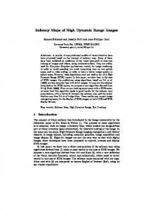
This project comprises an attempt to leverage the built-in numerical tools and rapid-prototyping facilities provided by Matlab to implement the system described in Paul Debevec's seminal paper 'Recovering High Dynamic Range Radiance Maps from Photographs.' This paper presents a method for constructing high-dynamic range radiance maps by combining a series of photographs, each of which contributes a portion of the total dynamic range. The built-in image processing facilities provided by Matlab have proven to make it an ideal tool for the implementation of this algorithm, as well as for constructing a simple GUI for experimenting with it. This GUI may be started by executing the command 'hdrView' from the Matlab console.

hdrView

2

The essential information required to construct the radiance map is a set of images with known exposure times. Such a set may be loaded into hdrView by pressing the LoadImages button and selecting as many images as desired. This images are assumed to represent a static scene and to be aligned to each other. Once the images are loaded the user may click on the "1/Shutter Speed" row in the Input Images table to enter the correct exposure time for that image. Alternatively, if the input file name contains the string '_s' followed by a set of digits, these digits are automatically taken to be the exposure time. Given this information, it is possible to construct the function which maps the amount of light received by the camera to the pixel values produced, and thus to reverse thus mapping to obtain the actual amount of light received at each pixel. This information can then be used to construct the radiance map from the set of individual photographs. See the references for the details of this process.

Two images from the sample input set Although the set of images and exposure times is all that is required to compute the radiance map, for reasons of computational efficiency it is desirable to identify a small sample of the total image which will be used in the computation. These sample points may be identified by using the built-in Matlab correspondence point tool (cpselect). Pressing the CP Tool button will launch this tool, showing two of the input images (one at low and one at high exposure). Points may then be identified on either image, the relationship between the points is not preserved, each one is taken to be an independent sample. Once points are specified they should be saved to the base workspace. They may then be imported into hdrView with the Import button. This will import any points defined in the variables input_points, base_points, and cpstruct in the base workspace (these are the default variables which cpselect saves to). It is worth noting that cpselect will save non-matched correspondence points only to the cpstruct variable, not to base_points or input_points, so it is important to save this variable when saving points. Alternatively, a set of points may be loaded from a .mat file, or randomly sampled from across the image. Once a set of points has been selected, it may be saved to a .mat file or exported back to the base workspace for later use.

3

Sample Point Selection Once a sufficient number of sample points have been defined, the characteristic function mapping radiance values to pixel values may be computed. This is done by pressing the appropriate button on the GUI, after which previews of the curves for each of the red, green, and blue channels, as well as a composite graph of the three will appear. It is also possible at this point to adjust the value of lambda, the smoothing constant used when computing the function. Full views of these curves may then be examined by clicking on the preview of the desired curve, which will cause it to load in a standard Matlab figure.

Characteristic Curves with lambda = 1

4

Characteristic Curves with lambda = 50 Following computation of the characteristic curves, it is possible to construct the high dynamic range radiance map. Clicking on 'View Linear Mapping' will cause this construction to take place, and the resulting image will be show in a Matlab figure. By default the entire image is linearly mapped to the descretized 0...255 values expected by a standard display. Due to the high dynamic range, this typically results in an extremely dark image, as the few high-intensity regions force the more wide-spread low-intensity regions into the same set of values at the bottom of the spectrum. To address this issue and make it possible to view the low intensity regions, it is possible to limit the display to the bottom x% of the total range. The final HDR image may also be saved back to the base workspace with the appropriate GUI button. This will assign the image to a variable named Ihdr, which may then be treated as a standard Matlab matrix..

Linear mapping of HDR images, using 100 % and 10 % of the total range. Given the newly constructed HDR image, it is desirable to be able to manipulate it outside of Matlab using other standard image processing tools. Unfortunately Matlab does not include support for any HDR formats. Thus the ability to write files to and read in the OpenEXR file format has been implemented. This has been implemented by writing a pair of MEX extensions which must be placed somewhere in the Matlab path (most conveniently in the current working directory). These extensions have been written and tested on Microsoft Windows, however they include no platform-specific code, so they should port to other platforms without problems. Making use of these extensions, it is possible to

5

save the generated image as an OpenEXR file, and view it with other tools, for example exrdisplay which is included in the standard OpenEXR distribution.

Views of the test scene after saving to an OpenEXR file This implementation of this project has been spread across a small set of files. gsolve.m is the original Matlab code included in Debevec's paper, and serves to find the least squares solution to the characteristic function. This on the only piece of third-party Matlab code used for this project. makeJavaTable.m contains a single function for creating a Java table which may be embedded in a Matlab figure. The rest of the implementation is contained in hdrView.m and hdrView.fig, which define both the user interface and all the code for constructing and manipulating the input images, HDR images, and other data structures required. The mexOpenEXR directory contains my MEX extensions which allow Matlab to use the OpenEXR library to read and write compressed HDR files. These make use of the OpenEXR and zlib libraries at run-time, thus it will not be possible to save or load EXR files if these libraries are not installed. The full source code for this project, as well as the sample dataset and precompiled MEX extensions may be retrieved from: http://people.ucsc.edu/~keller/cs060m/

References Debevec, P. E. and Malik, J. 1997. Recovering high dynamic range radiance maps from photographs. In Proceedings of the 24th Annual Conference on Computer Graphics and interactive Techniques International Conference on Computer Graphics and Interactive Techniques. ACM Press/Addison-Wesley Publishing Co., New York, NY, 369-378. DOI= http://doi.acm.org/10.1145/258734.258884