Jun 2, 1991 - Secondly, when training and testing on the same image, our method achieves competitive performance with. FR-IQA on the XT dataset [8].
BLIND HIGH DYNAMIC RANGE IMAGE QUALITY ASSESSMENT USING DEEP LEARNING Sen Jia
Yang Zhang, Dimitris Agrafiotis and David Bull
Intelligent Systems Laboratory University of Bristol
Bristol Vision Institute University of Bristol
ABSTRACT In this paper we propose a No-Reference Image Quality Assessment (NR-IQA) on High Dynamic Range (HDR) images using deep Convolutional Neural Network (CNN) combining with saliency map. The proposed method utilises the power of deep CNN architecture to extract quality feature which can be applied cross HDR and Standard Dynamic Range (SDR) domains. The saliency map is used to select a subset of salient image patches for CNN model to evaluate on. Our CNN-based method delivers state-of-the-art performance in HDR NR-IQA experiment, competitive with full reference IQA methods. Index Terms— HDR, No-Reference Image Quality Assessment, Deep Learning, Saliency Map 1. INTRODUCTION No Reference (NR) image (and video) quality metrics have until recently been associated with poor performance in estimating the perceived quality of an image or video [1]. Recently deep learning based NR metrics have been proposed for estimating the quality of images without any reference to the original [2, 3, 4]. These have produced some promising results, closing the gap to the performance offered by full reference methods. As with Standard Dynamic Range (SDR) images, Image Quality Assessment (IQA) for HDR images is more challenging and even more so when reference image is unavailable. This paper describes a deep learning method to NR-IQA for HDR images that offers performance very close to that achieved with Full Reference (FR) HDR quality metrics. Many of the existing deep learning based methods of NRIQA employ Convolutional Neural Networks (CNNs) to extract image features that are useful. For those CNN-based methods, the input image is split into multiple patches and a quality estimation is performed for each patch based on the features present in the patch. Kang et al. [2] proposed a shallow CNN architecture which contains one convolutional layer. Their method achieved competitive results with FRIQA on the LIVE [14] and the CSIQ [15] datasets. The authors extended this CNN architecture for NR-IQA and distor-
tion type classification in [3]. It has been proven that adding more layers to the CNN offers increases the feature extraction capability [5, 6, 7]. Compared to [2, 3], the method proposed in our paper employs a CNN with significantly more convolutional layers (ten as opposed to one layer). Recently Bosse et al. [4] proposed a CNN-based NR-IQA method also employing multiple layers. Their method utilises the power of deep CNN architecture but they try to solve the issue of equal weight patch by learning a weight parameter from the activation of rectified linear unit. The weight parameter is learned by CNN model itself such that the importance of a patch may not consistent with human vision systems. Our method attempts to solve the equal weight patch problem by utilising saliency map to guide a CNN model only evaluating on salient image patches. Unnoticeable qulity distortion in SDR range may become more obvious in HDR range [12]. Thus a tone-map is required to convert HDR image to SDR range for IQA. But crossdataset IQA on HDR is still challenging because luminance range is various from different datasets. Korshunov built a public HDR image dataset [8] on which Hanhart benchmarked most objective quality metrics [9]. The best FR-IQA on the XT dataset was HDR-VDP proposed by Narwaria [10] and the algorithm was designed for HDR content. After tonemapping HDR image to SDR, the algorithm of [11] achieved the best result in the domain of Perceptually Uniform (PU) [12]. For NR-IQA on the XT dataset, the method of [13] achieved the highest result in the both domains of HDR and PU. We compare our method with state-of-the-art FR and NR IQA on the same dataset. Another HDR dataset, JPEG [16], is also used to investigate the generalisability of our method. Firstly we train a CNN model on the LIVE dataset [14] to learn SDR quality feature. The trained model can extend SDR quality information on tone-mapped HDR image for NR-IQA. Secondly, when training and testing on the same image, our method achieves competitive performance with FR-IQA on the XT dataset [8]. Thirdly, we train our method on one HDR dataset and evaluate the peroformance on another HDR dataset. The experiment shows that our method can achieve good performance when directly applying on HDR images and further improvement can be achieved by
using the tone-mapping function of PU. 2. DATASETS AND METHODOLOGIES 2.1. SDR Datasets We use two SDR datasets in our experiment. The LIVE dataset [14], which contains 799 images with five types of distortion noise. The ground truth label for the LIVE dataset is Differential Mean Opinion Scores (DMOS) in the range of [0,99]. We train an SDR CNN model on the LIVE dataset and apply it on HDR datasets for cross-dataset experiment. The other SDR used in this work is CSIQ [15], whose label is also DMOS in the range of [0,1]. The CSIQ dataset is only used to evaluate the model trained on LIVE. 2.2. HDR Datasets Our experiment is mainly based on two HDR datasets, XT [8] and JPEG [16]. The XT dataset contains 240 distorted HDR images. While the JPEG dataset contains 150 distorted HDR images. The ground truth of the two HDR datasets is MOS in the range of [0,5]. We also convert the HDR datasets to SDR range by using the tone-mapping algorithm in [12]. The two tone-mapped datasets are referred as XTPU and JPEGPU respectively, see Section2.3.1. 2.3. Methodologies For each dataset, we local normalise every image using the algorithm in [2, 17]. Each image is split into small patches in the size of 32×32 assigned with the same label. Like the work of [4], we train a CNN architecture on those image patch. But the difference in our method is that we use saliency map computed on each image to assign weight for each patch instead of learning the weight from network activation. Two measurements are applied, Linear Correlation Coefficient (LCC) and Spearman Rank Order Correlation Coefficient (SROCC). 2.3.1. Tone-Mapping Comparing with SDR, HDR was designed to store a wider range of luminance value therefore an invisible distortion in SDR may become noticeable in HDR. To extend SDR quality metrics to HDR, Aydin [12] proposed a tone-mapping function that can apply SDR IQA methods on HDR, so called perceptually uniform encoding. Note that the mapping function between HDR and SDR is referred as tone-mapping in this paper to differentiate the logistic mapping applied for DMOS to MOS. 2.3.2. Local Normalization Following the same preprocessing protocol in [17, 2, 3], a contrast normalization has been applied on each image before
spliting into patches. This process might be important for cross-dataset evaluation between SDR and HDR. The pixel value range of a normalised image from either SDR or HDR is squashed into a small range centered at zero, as shown in Figure 1. 2.3.3. CNN Architecture Kang [2] used only one convolutional layer followed by maxpool and minpool layers. Our proposed CNN architecture is similar to [5, 4] that ten convolutional layers with small receptive fields are stacked: conv3-32, conv3-32, maxpool2, conv3-64, conv3-64, maxpool2, conv3-128, conv3-128, maxpool2, conv3-256, conv3-256, maxpool2, conv3-512, conv3512, fc2048, fc2048, softamx. The input image patch is 32 × 32 and the convolutional kernel is 3×3. A 2×2 maxpool layer is added and the number of kernels is doubled every two convolutional layers. Two fully connected layers are added at the end of the model, each of which has 2048 units. Dropout is added in the two fully connected layers with ratio of 0.5. We apply exponential linear units [18] after each convolutional and fully-connected layer. 2.3.4. Saliency Map To better mimic human vision systems, saliency map is utilised to select a subset of salient image patches to evaluabte on. We apply the algorithm of [19] to compute saliency map on SDR images and the algorithm of [20] on HDR. Every pixel value of an saliency map is rescaled to the range of [0,1]. We define the summation of pixel value within a saliency patch represents the importance of the image patch. P Ii =
m=M X−1 X−1 n=N m=0
s(m, n)
(1)
n=0
where M , N is the size of the patch, s(m, n) is pixel value of the saliency patch and P Ii is the importance for ith image patch in the range of [0,M × N ] (M = N = 32). We set a threshold θ to select a subset of salient image patches to evaluate on. The ith image patch is considered to be salient if its importance P Ii > θ × M × N . In our experiment the threshold is chosen from {0,0.01,0.1,0.5}. Note that when θ = 0, no saliency map is applied because all the image patch is considered to be salient. 3. EXPERIMENTS 3.1. SDR cross-dataset Our first experiment is to test if the quality feature learned from SDR distribution can generalise well on HDR images. An SDR CNN NR-IQA model is trained on all images from the LIVE dataset. The total number of training epochs is 15.
(a)
(b)
(c)
Fig. 1. Local normalised images. (a) Normalised LIVE image (SDR). (b) Normalised JPEG image (HDR). (c) Normalised JPEGPU image (SDR). The start learning rate is 0.001 and the momentum is 0.9 and they both reduce every five epoch by multiplying 0.1 and subtracting 0.1 respectively. We apply the model on the CSIQ dataset [15] to evaluate its SDR cross-dataset performance. No logistic mapping is applied because they both use DMOS for annotation. In Table 1, our method achieves 93.23% LCC and 93.31% SROCC when θ = 0.5. Which outperforms stateof-the-art SDR cross-dataset results in the papers of [17, 2, 3]. Table 1. Training on the LIVE dataset, testing on the CSIQ, XT, JPEG and their tone-mapped datasets. θ CSIQ-LCC CSIQ-SROCC XT-LCC XT-SROCC JPEG-LCC JPEG-SROCC XTPU-LCC XTPU-SROCC JPEGPU-LCC JPEGPU-SROCC
0 92.79% 93.21% 74.66% 74.50% 21.86% 23.99% 87.68% 86.42% 75.87% 75.17%
0.01 92.80% 93.21% 72.15% 73.42% 24.76% 25.87% 86.33% 86.10% 73.73% 73.75%
0.1 92.80% 93.31% 73.19% 73.67% 27.68% 30.39% 87.78% 87.38% 74.24% 73.45%
0.5 93.23% 93.31% 73.73% 72.96% 24.72% 25.26% 89.19% 88.49% 79.53% 79.81%
We then apply the model on the two HDR datasets to investigate the generalisability of the learned feature from SDR. A logistic mapping with five parameters [2] is applied to convert the output of the model from DMOS to MOS. Each of the two HDR datasets is split into two subsets, 80% of the total for training the mapping function and 20% is for evaluation. We shuffle and repeat this process ten times to report average accuracy. As shown in Table 1, the SDR model performs poorly on HDR images. Especially on the JPEG dataset, the highest average LCC is 27.68% and 30.39% on SROCC. On the tone-mapped image, 79.53% LCC and 79.81% SROCC were obtained on the JPEGPU dataset and the performance on the XT dataset is also increased. The model performs better on the tone-mapped image because the quality information
is learned from SDR dataset. 3.2. HDR within-dataset The second experiment is to investigate if HDR image can offer more quality information to train a model for HDR IQA. We do not use a logistic mapping in this experiment and afterwards since the two HDR datasets share the smae MOS label range. We firstly evaluate our method using within-dataset experiment setting that the training and test sets are from the same HDR dataset. For each of the two HDR datasets, we split it into 60% for training, 20% for validating and 20% for testing. The training protocol is the same as used on the LIVE dataset. In Figure 2, we show the average learning curve of ten splits on the validation set. Our method achieved over 90% accuracies on the validation set and saliency map (θ = 0.5) delivered a further improvement. During each split, Table 2. The average accuracy on the HDR test set. HDRVDP2-XT-LCC[9] 96.04% HDRVDP2-XT-SROCC[9] 95.64% MSSSIM Y-XTPU-LCC[9] 94.47% MSSSIM Y-XTPU-SROCC[9] 95.01% Marziliano Y-XTPU-LCC[9] 51.14% Marziliano Y-XTPU-SROCC[9] 41.79% Proposed-XT-LCC (θ = 0.5) 92.91% Proposed-XT-SROCC (θ = 0.5) 93.01% Proposed-JPEG-LCC (θ = 0.5) 87.99% Proposed-JPEG-SROCC (θ = 0.5) 88.87%
we record the highest test accuracy based on LCC achieved on the validtion set. The average accuracy on the test set of ten random splits is reported in Table 2 to compare with other methods. Note that the HDR-VDP [10] was only applied on HDR content because the algorithm was designed for absolute luminance values. The FR-IQA MSSSIM [11] and
Average performance on the XT-HDR validation set, ALL
0.95
0.90
0.94
0.88 Accuracy
Accuracy
0.93 0.92 0-LCC 0-SROCC 0.01-LCC 0.01-SROCC 0.1-LCC 0.1-SROCC 0.5-LCC 0.5-SROCC
0.91 0.90 0.89
Average performance on the JPEG-HDR validation set, ALL
0.92
0
2
4
6 8 Number of epochs
10
12
0.86 0.84 0-LCC 0-SROCC 0.01-LCC 0.01-SROCC 0.1-LCC 0.1-SROCC 0.5-LCC 0.5-SROCC
0.82 0.80 14
(a)
0.78
0
2
4
6 8 Number of epochs
10
12
14
(b)
Fig. 2. LCC and SROCC accuracies on the validation set using different importance coefficient (θ = [0, 0.01, 0.1, 0.5]). NR-IQA Marziliano [13] achieved better performance on the tone-mapped dataset. The proposed method achieves competitive result with state-of-the-art FR-IQA methods on the XT dataset, 92.91% LCC and 93.01% SROCC. 3.3. HDR cross-dataset In the second experiment we show that our method can be directly applied on HDR images. But the generalisability plays a very important role for CNN-based IQA methods. Let’s recall that there is no standard format of HDR luminance range. The learned quality feature by a CNN model may contain little in common with unseen HDR image. Therefore our third experiment is to train a CNN model on all images from one HDR dataset and test on the other, so called HDR crossdataset evaluation.
datasets following the same protocol used in the first experiment. We show the cross-dataset result on the two HDR datasets in Table 3. Using saliency map delivers a slightly better result but the highest accuracy (θ = 0.5) in Table 3 is worse than the within-dataset result in Table 2. It is interesting to see that the cross-dataset LCC and SROCC on the JPEG dataset are much higher than the SDR model obtained in Table 1. The HDR datasets share more common quality feature than it between SDR and HDR. But the CNN learned quality feature may still be dataset-specific when comparing with within-dataset experiment. To further bridge the gap of image format between the HDR datasets, we repeat the HDR cross-dataset experiment on the PU datasets. In Table 3, we can see that the performance has been increased significantly.
4. CONCLUSION Table 3. HDR Cross-dataset LCC and SROCC accuracies with different θ values. θ XT-LCC XT-SROCC JPEG-LCC JPEG-SROCC XTPU-LCC XTPU-SROCC JPEGPU-LCC JPEGPU-SROCC
0 73.22% 78.38% 78.62% 77.65% 86.37% 89.04% 85.51% 86.21%
0.01 73.26% 78.40% 78.94% 78.06% 86.35% 89.04% 85.54% 86.30%
0.1 73.29% 78.39% 79.05% 78.20% 86.31% 88.96% 85.48% 86.26%
0.5 73.12% 77.97% 79.33% 78.44% 86.34% 89.02% 85.09% 85.70%
Two models are trained seperately on the two HDR
In this papaer we proposed a NR-IQA method on HDR images using CNN and saliency map. We have proven that saliency map can further guide CNN when evaluating on HDR dataset. Our method can extend SDR quality information to tone-mapped HDR images for NR-IQA. When training and testing on the HDR dataset, our method has achieved competitive result with FR-IQA methods on the XT dataset. We further investigated the generalisability of our method by training and testing on different HDR datasets. Our method can be directly applied on HDR images to learn quality feature. A better performance can be obtained after tone-mapping HDR image to SDR.
5. REFERENCES [1] “No-reference image and video quality estimation: Applications and human-motivated design,” Signal Processing: Image Communication, vol. 25, no. 7, pp. 469 – 481, 2010, Special Issue on Image and Video Quality Assessment. [2] L. Kang, P. Ye, Y. Li, and D. Doermann, “Convolutional neural networks for no-reference image quality assessment,” in 2014 IEEE Conference on Computer Vision and Pattern Recognition, June 2014, pp. 1733–1740. [3] L. Kang, P. Ye, Y. Li, and D. Doermann, “Simultaneous estimation of image quality and distortion via multi-task convolutional neural networks,” in 2015 IEEE International Conference on Image Processing (ICIP), Sept 2015, pp. 2791–2795. [4] S. Bosse, D. Maniry, T. Wiegand, and W. Samek, “A deep neural network for image quality assessment,” in 2016 IEEE International Conference on Image Processing (ICIP), Sept 2016, pp. 3773–3777. [5] Karen Simonyan and Andrew Zisserman, “Very deep convolutional networks for large-scale image recognition,” Eprint Arxiv, 2014. [6] Christian Szegedy, Wei Liu, Yangqing Jia, Pierre Sermanet, Scott E. Reed, Dragomir Anguelov, Dumitru Erhan, Vincent Vanhoucke, and Andrew Rabinovich, “Going deeper with convolutions,” CoRR, vol. abs/1409.4842, 2014. [7] Kaiming He, Xiangyu Zhang, Shaoqing Ren, and Jian Sun, “Deep residual learning for image recognition,” CoRR, vol. abs/1512.03385, 2015. [8] P. Korshunov, P. Hanhart, T. Richter, A. Artusi, R. Mantiuk, and T. Ebrahimi, “Subjective quality assessment database of hdr images compressed with jpeg xt,” in 2015 Seventh International Workshop on Quality of Multimedia Experience (QoMEX), May 2015, pp. 1–6. [9] Philippe Hanhart, Marco V. Bernardo, Manuela Pereira, Ant´onio M. G. Pinheiro, and Touradj Ebrahimi, “Benchmarking of objective quality metrics for hdr image quality assessment,” EURASIP Journal on Image and Video Processing, vol. 2015, no. 1, pp. 39, 2015. [10] Manish Narwaria, Rafal Mantiuk, Matthieu Perreira Da Silva, and Patrick Le Callet, “Hdr-vdp-2.2: a calibrated method for objective quality prediction of high-dynamic range and standard images,” J. Electronic Imaging, vol. 24, pp. 010501, 2015. [11] Z. Wang, E. P. Simoncelli, and A. C. Bovik, “Multiscale structural similarity for image quality assessment,”
in The Thrity-Seventh Asilomar Conference on Signals, Systems Computers, 2003, Nov 2003, vol. 2, pp. 1398– 1402 Vol.2. [12] TunC¸ Ozan Aydın, Rafał Mantiuk, and Hans-Peter Seidel, “Extending quality metrics to full dynamic range images,” in Human Vision and Electronic Imaging XIII, San Jose, USA, January 2008, Proceedings of SPIE, pp. 6806–10. [13] A. V. Murthy and L. J. Karam, “A matlab-based framework for image and video quality evaluation,” in 2010 Second International Workshop on Quality of Multimedia Experience (QoMEX), June 2010, pp. 242–247. [14] H. R. Sheikh, M. F. Sabir, and A. C. Bovik, “A statistical evaluation of recent full reference image quality assessment algorithms,” IEEE Transactions on Image Processing, vol. 15, no. 11, pp. 3440–3451, Nov 2006. [15] Damon M. Chandler, “Most apparent distortion: fullreference image quality assessment and the role of strategy,” Journal of Electronic Imaging, vol. 19, no. 1, pp. 011006, jan 2010. [16] Manish Narwaria, Matthieu Perreira Da Silva, Patrick Le Callet, and Romuald Pepion, “Tone mapping-based high-dynamic-range image compression: study of optimization criterion and perceptual quality,” Optical Engineering, vol. 52, no. 10, pp. 102008–102008, 2013. [17] Peng Ye, Jayant Kumar, Le Kang, and David Doermann, “Unsupervised feature learning framework for no-reference image quality assessment,” in Computer Vision and Pattern Recognition (CVPR), 2012 IEEE Conference on. IEEE, 2012, pp. 1098–1105. [18] Djork-Arn´e Clevert, Thomas Unterthiner, and Sepp Hochreiter, “Fast and accurate deep network learning by exponential linear units (ELUs),” CoRR, vol. abs/1511.07289, 2015. [19] Hae Jong Seo and Peyman Milanfar, “Static and spacetime visual saliency detection by self-resemblance,” Journal of Vision, vol. 9, no. 12, pp. 15, 2009. [20] W. Zhang, A. Borji, Z. Wang, P. Le Callet, and H. Liu, “The application of visual saliency models in objective image quality assessment: A statistical evaluation,” IEEE Transactions on Neural Networks and Learning Systems, vol. PP, no. 99, pp. 1–13, 2016. [21] Amin Banitalebi-Dehkordi, Yuanyuan Dong, Mahsa T. Pourazad, and Panos Nasiopoulos, “A learning-based visual saliency fusion model for high dynamic range video (lbvs-hdr).,” in EUSIPCO. 2015, pp. 1541–1545, IEEE.