seconds. The objective of this paper is to explore and investigate time driven simulation models ... There exist three common models to simulate projectile in .... position of projectile given initial Velocity as âVâ and initial angle âthetaâ. It is important to note that Y(t) depends on X(t). III. LINEAR DRAG TRAJECTORY MODEL.
(IJACSA) International Journal of Advanced Computer Science and Applications, Vol. 9, No. 12, 2018
Recurrence Relation for Projectile Simulation Project and Game based Learning Humera Tariq1, Tahseen Jilani2, Usman Amjad5 Department of Computer Science University of Karachi Karachi, Pakistan
Ebad Ali3
Syed Faraz4
School of Computing National College of Ireland Dublin, Ireland
Center for Intelligent Signal and Imaging Research (CISIR) Universiti Teknologi Petronas Perak, Malaysia
Abstract—Huge Gap has been observed on study of projectile simulation models relating it to speed of camera or frame per seconds. The objective of this paper is to explore and investigate time driven simulation models to mimic projectile trajectory; with an intent to highlight importance of game programming on native platforms. The proposed projectile recurrence relation and extensive mathematical modeling based on Triangular Series is an innovative outcome of project and game based learning used in BSCS-514 Computer Graphics Course at Department of Computer Science (DCS) University of Karachi (UOK). Box2D Replica of Popular 2D Mobile Game Angry Bird has been created on desktop to have an in depth mathematical and programming insight of commercial physics engine and discrete event simulation. Analysis has also been performed to answer certain key questions for progressive projectile trajectory for e.g. (1) With What angle, projectile should be launched? (2) What is the maximum height it will reach? (3) How long it will take for landing? (4) What will be its velocity to reach a desired height? (4) Where it will hit? (5) How it will bounce? The above stated questions are important to answer so that projectile motion within engineering, Gaming and other CAD Applications can be taught and programmed correctly specially on native platforms like OpenGL. Besides reporting Numerical results, a successful projectile based game making has been compiled and reported to validate the significance of project based learning in classrooms and labs. Keywords—Projectile; game programming; simulation; angry birds; linear drag; trajectory; impulse
I.
INTRODUCTION
Understanding projectiles in an interdisciplinary manner is exceedingly important at variety of levels to incorporate them in real life applications. Engineering applications involving projectile use deep and precise analytical equations which are difficult to grasp and requires an in depth domain knowledge [1][2][3]. Classical literature documented Physical class room experiments to study and build understanding about projectile models [4][5]. CAD and gaming applications requires the same background knowledge along with programming skill for simulation and visualization of projectile trajectory. In this paper, an attempt to unlock the projectile behavior of available game development platforms from simulation perspective on computers. Platforms are available to facilitate engineers and programmers for building these physical models without handling the pressure of complex analytical mathematics and statistics. As a senior computer science faculty, I strongly
believe that understanding these mathematical foundation has played an immense important role in polishing ones‟ cognitive, engineering and programming skills [6] - [12]. There exist three common models to simulate projectile in computer applications for gaming and simulation; they are: (1) No drag model (2) Linear drag model and (3) Quadratic drag model. In no drag model, the motion of projectile is mainly dependent on initial velocity and the angle of launch. On the other hand, both linear and quadratic drag model taken into account, the air resistance effect on projectile trajectory. Demonstration of projectile has been done through replica of famous angry bird game using Box2D [13] [14] and figure out that which model has been used in this physics engine? Rest of the paper is organized as follows: Section II and III discuss standard No drag and linear drag trajectory models respectively. Section IV till Section VII comprise of extensive derivations based on recurrence relation, triangular numbers and Frames Per Second Criteria (FPS). The derivations are inspired by Box2D and OpenGL experiments discussed in [13] -[17]. Experiments on spread sheet and through game programming has been discussed in Section VIII which follows Results and Discussion described in Section IX. Conclusion and Future Work has been presented in the end of this paper. II. NO DRAG TRAJECTORY MODEL In general, the motion produced by a body which follows projectile trajectory reached a certain elevation and then allow to descending as a mirror of elevation. The vector of the motion can be divided into two components, „x‟: the horizontal component and „y‟: the vertical component of the motion. The force at the horizontal vector remains unchanged throughout the motion while the vertical forces applied at the birds frequently changes due to the effect of gravity and height of the bird. For computing the velocity of the birds during the flight time, following equation can be used.
Vx V0Cos
(1)
Vy V0 Sin gt
(2)
The acceleration of the object, in both the components of motion remains constant throughout the flight time. Horizontal component of acceleration remains equal to zero and negative gravitational value at vertical . During flight
500 | P a g e www.ijacsa.thesai.org
(IJACSA) International Journal of Advanced Computer Science and Applications, Vol. 9, No. 12, 2018
time, highest point of the bird can achieve with the given initial angle and velocity applied
h V
Sin 2
2 0
(3)
2g
Equation (3) will compute the height of the flight with respect to the ground. Range of the projectile launched is also important to calculate because this information will enable us to determine the landing position of the object. The mathematical model for computing total range of the bird is mentioned below 2
R Vx
Sin 2 2
g
(4)
Range of the bird depends on two independent variables in the projectile motion of a game, first is the adjusted angle and second is the adjusted velocity of the bird. The angles of the launch greatly affect the range of the bird due to the trigonometric function of Sine on the angle. It is computed that at any velocity the bird will achieve the maximum range ( ) in Eq value if the angle adjusted is 450 because of (4). When the value of is equal to 45 then becomes equal to 90 degrees and thus maximum range will be 2
R Vx g
(5)
From simulation perspective, total time of flight is calculated by manipulation of Eq. (2) and Eq. (3) and finally putting h =0 to attain maximum range at ground. It is not difficult to have following equation for computation of total time of flight „T‟ in advance as follows
decomposed into its components along x and y-axis. The area for dragging the object is specified with reference to the initial position of the projectile. The drag backward is restricted on x-axis; the same will be true for y-axis. Drag displacement will be directly proportional to drag force. . If represents the change in distance due to drag then
F d
(9)
Eq (9) can be decomposed into two independent equations with respect to x and as follows:
Fx d x
;
Fy d y
(10)
The objective is to find final velocity with the help of initial velocity so that we can determine the launch speed with which it moves along projectile trajectory. Assume fixed time incremental approach with = 1. Assume that the Forces will remain constant throughout the projectile motion. The body will then move with uniform acceleration on x-axis. The y-component of launch velocity will be affected by the acceleration due to gravity g. The expression for final velocity along x-axis can be formulated as follows
Fx max
;
Fx m(V2 x V1x )
Fx (V2 x V1x ) m Fx V1x V2 x m
V2 x
Fx V1x m
(11)
Along y-axis; following simplified drag model has proposed to determine final velocity progressively
V T 2* y g
(6)
Once total time of flight is calculated, computation of points (X, Y) on trajectory will become possible by dividing time T into small equal space intervals t +delT as follows
X (t ) V x * t
Y (t ) X (t ) tan
(7)
1 1 ( 2 ) X (t ) 2 2 g V Cos 2 0
Fy ma y gt
(12)
Aa per our assumption, the change in momentum of projectile can be compared with change in vertical forces as follows
Fy m(V2 y V1 y ) gt Fy gt m(V2 y V1 y )
(8)
Eq (7) and Eq (8) are used to determine instantaneous position of projectile given initial Velocity as „V‟ and initial angle „theta‟. It is important to note that Y(t) depends on X(t). III. LINEAR DRAG TRAJECTORY MODEL Linear impulse is defined as a linear force applied on anybody i.e. . In many games, an external backward force is applied on body before launching it as projectile for e.g. drag of the bird in game “Angry bird” is applied through a slingshot controlled by user. This drag force will of course be
V2 y
Fy gt m
V1 y
(13)
IV. RECURRENCE RELATION FOR HEIGHT Our recurrence relation is inspired by Box2D description on projectile [13 [14]. To derive a general formula, that can be used to find the final velocity ( ) at any given point in time; each velocity assume to contain the sum of all the previous velocities. In a general way the velocities are in the arithmetic progression manner. If we use Eq (14) at each frame display in
501 | P a g e www.ijacsa.thesai.org
(IJACSA) International Journal of Advanced Computer Science and Applications, Vol. 9, No. 12, 2018
games, then the general expression for finding the height at any instant can be figure out by working from Eq (14) till Eq (17) Fy g ( V2 y (1)
V2 y ( 2 )
V2 y ( 3)
m
0 {ntotal
3 ) fps
m
ntotal
m
2 ) fps
Fy g (
1 ) fps
m 1 3 2 1 ( Fy g ( ) Fy g ( ) Fy g ( ) m fps fps fps
Fy
g g g 3 2 1 {1 ( ) 1 ( ) 1 ( )} m Fy fps Fy fps Fy fps
V2 y ( 3)
Fy m
{3
Fy m
{n
(19)
g 3 g 2 g 1 ( ) ( ) ( )} Fy fps Fy fps Fy fps
n
i i 1
ntotal
n(n 1) 2
(15)
If we use Eq(15) to find instant launch speed and we are given the initial height of the projectile then following equation can be used to find the height at any instance of time: H n V2 yn H 0
2 fps
Fy g
1 2 fps
(16)
This above equation can be further expanded into Eq (17) as we substitute final velocity from Eq(15). Here represents the initial height of the projectile at which it was launched
(20)
ntotal (ntotal 1) g 2 ( ) Fy fps
i
g i 1 ( )} Fy fps
n(n 1) 2
because this series is the nth partial sum of the series of triangular numbers.
n
V2 y ( n )
i g i 1 ( ) Fy fps
The sign of summation can be interchanged by
Fy g (
g i 1 ( )} Fy fps n
(14)
3 Fy g ( ) fps V1 y ( 2 ) m
V 2 y ( 3)
V 2 y ( 3)
V1 y ( 0 )
2 Fy g ( ) fps V1 y (1) m
Fy g (
V2 y ( 3)
1 ) fps
n
i
ntotal
ntotal 1
Fy g
ntotal
g 2 fpsFy g (21)
n
Hn
Fy m
{n
i g i 1 ( )} H 0 Fy fps
VI. RELATING VELOCITY AND HEIGHT (17)
Where i is the counter to track time instants while projectile is flying above the ground.
The derivation to find the velocity at the maximum height will follows from Eq (22) till Eq (25). Substituting time of flight from Eq (20) into Eq (15) of final velocity, we will get Eq (22)
V. TIME OF FLIGHT AS TRIANGULAR SERIES The total time for the flight of the projectile can be obtained by substituting final velocity as zero because the projectile will come to rest as it hits the ground, therefore where is used to represent instantaneous time of flight n
V2 y ( n )
Fy m
{ntotal
i
g ( i 1 )} Fy fps n
0
Fy m
i
{ntotal
g i 1 ( )} Fy fps
(18)
V2 y ( n )
Fy m
{n
g n(n 1) ( )} Fy 2 fps
(22)
Eq (20) provides the total time of flight but maximim height will be achieved at half time of the total therefore Eq (21) will turn into Eq (23) as follows
n1
( Fy )( fps) g
2
Assuming
g
(23)
x ( fps) Fy g ; Eq (23) become
502 | P a g e www.ijacsa.thesai.org
(IJACSA) International Journal of Advanced Computer Science and Applications, Vol. 9, No. 12, 2018
n1 2
VII. IMPULSE FORCE AND FINAL VELOCITY
x g
The equation for the final velocity due to the impulse force will be considered as follows
Substituting above fact into Eq (22), We have
V2 y
V2 y
V2 V1 (a g )t
x 2 xg ) 2 fps( Fy x) 1 g2 {g ( )} m 2 fps (
V2 y
(
x 2 xg 2 fps( Fy x) g 2 g2 2 fps
)
V2 y
V2 y
2 2 1 x xg 2 fps( Fy x) g {( )} m 2 fpsg
V2 y
V2 y V2 y V2 y V2 y V2 y
x {( m
2 fpsg
( fps) Fy g m ( fps) Fy g m ( fps) Fy g m
{(
)}
S4 V1 (a g )(3) V1 (a g )(2) V1 (a g )(1) V1 (a g )(0)
S n (n 1)V1 (a g )i 1 i n
Converting
)} (24)
( fps) Fy g g 2 fps( Fy ) g 2 2 fpsg
( fps) Fy 2 fps( Fy ) g 2 2 fpsg
{(
( fps) F y (1 2 g )
{(
2 fpsg Fy (1 2 g 2 ) 2g
)}
n
i 1
(27)
i notation to the general formula of
triangular series n(n 1) 2
S n (n 1)V1 (a g )
n(n 1) 2
(28)
The total time taken by the body to complete its trajectory where the velocity of the body becomes equal to zero. The equation for total time taken for the flight is as follows:
)}
S n (n 1)Vi (a g )
n(n 1) 2
n(n 1) 2 n 0 (n 1){Vi ( g a) } 2
)}
0 (n 1)Vi (a g )
)}
n 0 {Vi ( g a) } 2
{( fps) Fy g}{Fy (1 2 g 2 )} 2 gm
S 2 V2 V1
S 4 V4 V3 V2 V1
2
( fps) Fy g m
{(
S1 V1 ;
S 3 V3 V2 V1
1 {g ( m
x g 2 fps( Fy ) g 2
(26)
Where is the final velocity which is the consequence of the initial impulse, and is the initial velocity, is the acceleration provided to the body whereas represent the force of gravity applied on the motion of the body. This equation only tells us about the instantaneous velocity of a body at any given time. Indeed, apart from calculating the velocity, we are more interested in getting the current displacement at y-axis by the body with a given value of velocity. For e.g. What will be the distance covered by the body when and ? In this scenario, it can be said that every displacement is dependent upon the previous displacement that is why the following equation is given to fulfill our requirement.
x x ( 1) 2 fps( Fy x) Fy g g g { ( )} m Fy 2 fps( g ) x x ( 1) 2 fps( Fy x) 1 g g {g 2 ( )} m 2 fps( g ) 2
V2 y
V2 V1 at gt
x x ( 1) Fy x g g g { ( )} m g Fy 2 fps
(25)
Eq (24) and Eq (25) respectively represent the relation which represent velocity of projectile with respect to displayed frame in game and illustrate frame animation.
2Vi ( g a)n
;
Vi ( g a)
n 2
2Vi 2Vi n; n ( g a) ( g a)
29
503 | P a g e www.ijacsa.thesai.org
(IJACSA) International Journal of Advanced Computer Science and Applications, Vol. 9, No. 12, 2018 TABLE I.
The equation for calculating the maximum height achieved by the body during the flight is derived by substituting EQ (29) into EQ (27) as follows
S max
Vi Vi ( 1) Vi ( g a) ( g a) ( 1)Vi (a g )( ) ( g a) 2
S max
V (V g a) V (V g a) ( i i )( i i ) ( g a) 2( g a)
S max
2{Vi (Vi g a)} Vi (Vi g a) 2( g a)
Smax
V (V g a) i i 2( g a)
(30)
VIII. EXPERIMENTATION A. Spread Sheet Simulaiton of Pojectile Trajectory The purpose of spread sheet simulation is to visualize and test our proposed linear impulse based recursive projectile model. We already discussed Linear Drag Model in Section III. The force along x-axis is assumed to be constant according to our simulation assumption. The required initial parameters are set as follows for demonstration purpose
V
SIMULATION SAMPLE EQ (11)
V
1x
0
0.086957
0.086957
2
0.08695652
0.173913
0.173913
3
0.17391304
0.26087
0.26087
4
0.26086957
0.347826
0.347826
5
0.34782609
0.434783
0.434783
6
0.43478261
0.521739
0.521739
7
0.52173913
0.608696
0.608696
8
0.60869565
0.695652
0.695652
9
0.69565217
0.782609
0.782609
10
0.7826087
0.869565
0.869565
11
0.86956522
0.956522
0.956522
12
0.95652174
1.043478
1.043478
13
1.04347826
1.130435
1.130435
14
1.13043478
1.217391
1.217391
15
1.2173913
1.304348
1.304348
16
1.30434783
1.391304
1.391304
SIMULATION SAMPLE EQ (13), EQ (17)
V
It has been observed from Table 1 and Table 2 that the generated impulsive force has enough large magnitude over a very small interval of time (fraction of a second) that it causes a significant change in the momentum which in turn lift the projectile up in the air in response to initial drag during its flight. To build simulation start with ; compute as described in Eq (11)
2x
1
TABLE II.
With above initial conditions we use Eq (11) and Eq (13) to update velocity along each axis respectively at each frame or display of projectile. For simplicity, the change in time between frame displays is taken to be unit which means that time instances are taken as a fraction of 60. Table 1 and Table 2 Presents Numerical Results of progression in velocity along each axis. From Table 1, it has been observed, that the projectile is moving with uniform acceleration along x-axis as the difference between two adjacent velocities remained a constant.
V
1 .1
1y
V
2y
1
0.016
0
36.5217391
0
2
0.033
36.52174
72.1913043
36.52174
3
0.05
72.1913
107.008696
72.1913
4
0.066
107.0087
140.973913
107.0087
5
0.083
140.9739
174.086957
140.9739
6
0.1
174.087
206.347826
174.087
7
0.116
206.3478
237.756522
206.3478
8
0.133
237.7565
268.313043
237.7565
9
0.150
268.313
298.017391
268.313
10
0.166
298.0174
326.869565
298.0174
11
0.183
326.8696
354.869565
326.8696
12
0.200
354.8696
382.017391
354.8696
13
0.216667
382.0174
408.313043
382.0174
14
0.233333
408.313
433.756522
408.313
15
0.25
433.7565
458.347826
433.7565
16
0.266667
458.3478
482.086957
458.3478
504 | P a g e www.ijacsa.thesai.org
(IJACSA) International Journal of Advanced Computer Science and Applications, Vol. 9, No. 12, 2018
B. Spread Sheet Simulation of Time as Triangular Series It has been observed that current displacement of projectile can be seen as series of instantaneous velocities sum together where each instant can take the form of triangular number in series. The simulation sample of model described in Section VII is illustrated in Table 3 below. Some initial parameters for demonstration purpose are given following values *
TABLE III. t
g/(Fy*FPS)t
0 1 3 6 10 15 21 28 36 45 55 66 78 91 105 120
0 -0.023333 -0.07 -0.14 -0.233333 -0.35 -0.49 -0.653333 -0.84 -1.05 -1.283333 -1.54 -1.82 -2.123333 -2.45 -2.8
(
+
)
SIMULATION SAMPLE EQ (22) n+ g/(Fy*FPS)t 0 0.976666667 1.93 2.86 3.766666667 4.65 5.51 6.346666667 7.16 7.95 8.716666667 9.46 10.18 10.87666667 11.55 12.2
Fy/m* (g/(Fy*FPS)t 0 0.594492754 1.174782609 1.740869565 2.292753623 2.830434783 3.353913043 3.863188406 4.35826087 4.839130435 5.305797101 5.75826087 6.196521739 6.62057971 7.030434783 7.426086957
Fig. 1. Background Modeling and Translation Concept.
Fig. 2. Foreground Entities of Game as Textured Polygon.
C. Projectile Simulation on Box 2D and OpenGL Game Programming is an important and impressive tool to practice simulation. Box2D is used to simulate core projectile functionality whereas OpenGL „freeglut‟ library on windows is used for rendering and to interact with user through mouse and keyboard. Box2D modeled projectile as linear impulse force [13] [14]. The 2D game pipeline consist of following minimal basic steps to experiment with projectile. (1) Modeling (2) Animation (3) Collision Detection. Modeling of game world means setting up background and foreground. Background is indeed a flat polygon with height of 480 and width of 1920 pixels. The wide polygon is split into smaller polygon to be used as textured sheet. Fig. 1 demonstrate simple UV mapping on a rectangle to model background comprising of clouds, grassy land, and sun. So textured polygon made it convenient for a programmer to have nice background using glossy images. Fore ground entities Comprises of main characters such as Birds, Pigs, walls (Boxes) and slingshot. Game Characters are designed with simple polygons and we employ uv mapping to animate characters. These characters are represented by Bitmap images as shown in Fig. 2. As a matter of fact, all foreground objects are modelled at origin; later they are translated to specific position by using coordinate system transformation as illustrated in the for the Bird. The land type and background in the game need to change as projectile launces and trying to hit the target at distance ahead of its current position. This effect is achieved by setting predefined multiple polygons shown in Fig. 3 as Polygon A, B and C. When the game starts, user will able to see the initial background but when it uses sling shot to launch projectile, the coordinates get changed and user will experience change of background at the output screen. These multiple lands or polygons will be visible to the user at its screen and the view will be updated at runtime. Foreground modeling is another important part of the game as they will change with their state on different triggers and events. All Game character (birds), pigs (enemy), boxes, hurdles and other bitmaps are counted as foreground elements. The foreground is divided into two section of the screen. The left portion of the foreground is dedicated for modeling the slingshot and the birds which are in the control of the user. This portion will enable the user to adjust the angle and the speed for launching the birds at a trajectory of projectile motion through the slingshot in order to hit the walls and to eliminate the pig. The other portion of the foreground consists of the defensive walls for the pigs. All the Birds in game are modeled by drawing circles and then applying bird texture on them. While Boxes and slingshots are modeled by applying texture on to the rectangles. When the game is initialized, all the characters and the objects in the game are drawn at the initial position of the screen, at (0, 0). The positions of these various models in this game are translated with respect to their functionality and behavior, as the initial bird is set near the slingshot elevated by default ready to be shot by the user, on the other hand other birds wait for their turn in a row wise manner. The pigs are modeled in between the walls or the boxes on the other side of the screen.
505 | P a g e www.ijacsa.thesai.org
(IJACSA) International Journal of Advanced Computer Science and Applications, Vol. 9, No. 12, 2018
Fig. 3. Wide Polygon Design to Map Levels in Game.
Physics played a vital role in animation of all characters. Following aspects need to be considered in order to model the desired animation. (1) In which direction it should be launched to meet the desired result? (2) How high it will go? (3) How long it will take to land on the floor? (4) Where it will hit the ground? (5) How far away from the ground? (6) Collision Detection. Slingshot is used in this game in order to set the launching direction and to make accurate shot at the pigs. The slingshot uses the birds for attacking pigs confined in a defensive wall. The slingshot is animated with the help of mouse events and buttons. Slingshot is stretched with the left button of the mouse for adjusting the force or the speed and the angle at which the bird will be shot. The right button is used to launch the bird at the pigs with the angles and the force adjusted earlier. Birds being shot through the slingshot are translated at an angle with an initial velocity and become projectile under the influence of gravity. The animation of the bird is handled according to trajectory model already described in detail from Eq (1) till Eq (13). Observe the arrangement of Woods in Fig 4. Falling of wood Boxes is established under the acceleration due to gravity and is achieved by using Newton‟s second equation of motion. But, the initial velocity Therefore, the rate at which body is falling is: Another Noticeable construct is once again the application of parametric equation to generate points on the curve as already described in Eq (7) and Eq (8). After modeling and animation, the last aspect of a basic 2D game is to detect collision between entities. Principal of Separating Axis Theorem (SAT) states that: “If two convex objects are not penetrating, there exists an axis for which the projection of the objects will not overlap.” To detect whether two objects are being collided, projection of their axis are calculated. If the distance between all the projections is equals to or less than zero, then it is said that the object has collided with each other. If projection of bird overlaps with projection of box on both horizontal and vertical, animation event is triggered. This concept has been extended and applied on every polygon as shown in Fig. 5.
Fig. 4. Animation to Show Fall of Woods or Boxes.
One can note that how a 2D collision detection problem can be transformed into 1D problem. Orange and Blue Lines in Fig. 5. are Projection of Polygons A and B on axes respectively. Black Line represents the Portion on the line where a plane can be inserted separating A and B. Two steps are needed to perform SAT: (1) Finding axis (2) Projection of shapes (3) Collision detection. Axes are simply normal of each shape‟s edges. This can be calculated by subtracting the vertices of the respective edges and then taking perpendicular of it as show in the Pseudocode of Table 4. Projecting shapes onto Axes and then comparing overlapped portion of the projection would result in Collision Detection. Pseudo code in Table 5 models this idea
Fig. 5. Overlapping Projections for Collision Detection. TABLE IV.
FINDING AXIS BY VECTOR SUBTRACTION
for all Edges in A P1 = First Vertex of A P2 = Second Vertex of A Vector edge = P1.subtract (P2); Vector normal = edge.perp (); // Axis arrayOfAxis.add (normal); end for
TABLE V.
COLLISION DETECTION BY OVERLAPPING TECHNIQUE
for all Shapes in S for all Axes of S in A Projection p1 = s.project (A); Projection p2 = s2.project (A); // s2 is the second shape. if (!p1.overlap(p2)) return false; end for Axes end for S
IX. RESULT AND DISCUSSION Successful Simulation of extensive mathematical models has been demonstrated using both Spread Sheet and C++ programming by integrating Box2D and OpenGL. Fig. 6 shows the result of applying impulse force as agent at initial time of the motion, after which the velocity produced by this impulse and force of gravitation contributes for further movement of the projectile. In our scenario the impulse is being applied at the center of the body. The y-component of the force mimics the angle of launching the projectile towards the target while x-component is the linear force or speed with which the bird is supposed to launch. FPS is 60 frames per
506 | P a g e www.ijacsa.thesai.org
(IJACSA) International Journal of Advanced Computer Science and Applications, Vol. 9, No. 12, 2018
second and is the rate at which box2D updates or refreshes its View Window. Fig. 7 shows that it is possible that flight time will take form of triangular series and the projectile trajectory is successfully followed if triangular increment is used for simulation. The simulation of linear impulse in box2D and OpenGL requires two arguments: (1) An initial vector V0 containing and component of velocity (2) A Point from where impulse has to be triggered. Y-component of final velocity is denoted with ( ) i.e. velocity at time instance t in future; g is 9.8 m/s, „F‟ represents y-component of force applied on mass „m‟. FPS is defined as the default frame per second value of box2D which is 60. Reciprocal of „FPS‟ provides us with time to render single frame which in turn plot the position of body. To mimic original game, projectile is fired and controlled through mouse pointer. To aim pigs at a certain angle; birds are controlled by click buttons of the mouse. Left button is used for adjusting speed value of the bird whereas the right button controls the angle of the shot being made. All the variable setup is shown in Fig. 8 for reader convenience. By using Mouse interactions with the system we developed multiple techniques to deal with the angle, at which the bird would fly, and magnitude of force, with which the bird would be fired, from the slingshot. The movement of mouse on the horizontal axis (xFactor) would modify the magnitude of force by some fraction. Similarly, the vertical displacement (yFactor) would intervened the angel of flight by some value as shown in the Fig. 9. In the end we have presented a comparison of OpenGL and Box2D simulation loop in Table 6.
Fig. 6. Simulation Result of EQ (17) Recurrence Relation of Projectile Height as a Function of Projectile Final Velocity and Frame Per Second.
Fig. 7. Simulation Result of EQ (22) Where Flight Time Takes the form of Triangular Series and Mimics Projectile.
Fig. 8. Simulation Settings of Projectile Linear Drag Model using Box2D and GLUT API.
Fig. 9. Mapping of Mouse Drag Action in Game onto Impulse Force (xFactor) and Angle of Projectile (yFactor).
507 | P a g e www.ijacsa.thesai.org
(IJACSA) International Journal of Advanced Computer Science and Applications, Vol. 9, No. 12, 2018 TABLE VI.
COMPARISON OF GLUT AND BOX2D SIMULATION LOOP
OpenGL (glut) Simulation Loop
Box2D Simulation Loop Step 1 Creation of World Create a gravity vector Create Global b2world object with gravity vector
Step 1 System-dependent initialization • setup a window on the screen • bind OpenGL to this window Step 2 OGL and CS initialization • setup coordinate system • setup initial values Step 3 Begin eternal loop • wait for system to deliver event (e.g., mouse moved)
Step 2
• If redraw event, execute OpenGL commands to draw scene by calling Draw ()
[5]
X. CONCLUSION AND FUTURE WORK Replica of popular angry bird game has been successfully implemented during BSCS-Computer Graphics class project at Department of computer Science, University of Karachi. Integration of physics engine Box2D and OpenGL on Visual Studio and windows platform has been successfully achieved. Linear Drag Simulation on Spread Sheet doesn‟t exactly match with functionality available in Box 2D and hence It has been concluded that mathematical modeling and simulation is an essential ingredient of learning which cannot be excluded from class environment due to easy access of commercial engines and open source libraries. Instead it is very important to exercise elementary pipeline of engines as a class project. This will enhance one‟s programming skills and also inculcate bottom up approach for building innovative software‟s either on the top of existing one or by developing it from scratch. Future work will comprise of dimension analysis of drag model presented in this paper. The work is also extended by demonstration of projectile using Vulkun API instead of glut or free glut with intention of handling physics and rendering in separate threads for effective GPU utilization. [1]
[2] [3]
[4]
Creation of Bodies Create body object Insert it into the world Create its fixture Create a shape for the fixture Assign the fixture to the body Step 3 Rendering of world‟s Bodies For all bodies n in the world { Draw n }
REFERENCES Semih M.Olcmen, Gray C.Cheng, Richard Branam and Stanley E Jones. “Minimum drag and heating 0.3 caliber projectile nose geometry.” doi: 10.1177/0954406218779094 G.P.de Carpentier, “Analytical ballistic trajectories with approximately linear drag”, Int. J. Comp. gam. Tech.2014. O.A. Lasode , O.T.Popolla, Olaleya. “Modeling the Projectile Motion of a soccer ball under linear drag influence” J. Research Info. Civil Engg, Vol 6, No.2 2009. P.Coutis, “Modelling the prpjection motion of a cricket ball”, Int. J. Math. Edu. Sci. Tech., vol. 29, pp.789-798, 2006.
[6]
[7]
[8]
[9]
[10] [11]
[12]
[13] [14] [15] [16]
[17]
N.Azarnia, “A progression of projectiles: examples from sports”, The Coll. Math. J., vol.25, no.05, pp.436-442,1994. J.Yang, G.K.W.Wong and C.Dawes, “An exploratory study on learning attitude in computer programming for the twenty-first century”, N. Med. Edu. Change, pp.59-70, 2018. F.J.G.Penalvo and A.J.Mendes, “Exploring the computational thinking effects in pre-university education”, Comp. Hu.Behav., vol.80, pp.407411, 2018. M.J.Nathan, M.Wolfgram, R.Srisurichan, C.Walkington and M.W.Alibali, “Threading mathematics through symbols,sketches,software,silicon and wood: Teachers produce and maintain cohesion to support STEM integration”, J. Edu. Res., vol.110, no.3, pp.272-293, 2017. M.J.Rodrigues and P.S.Carvalho, “Teaching physics with angry birds: Exploring the kinematics and dynamics of the game”, Phy. Edu., pp.431-437, 2013. R.Bidarra, “Interdisciplinary game project: Opening the graphics (Back) door with the soft skills key”, Edu. Paper, p.9-16, 2011. M.Shaker,N.Shaker and J.Togelius, “Evolving playable content for cut the rope through a simulation-based approach”,proc.9th AAAI conf. on AI and interactive digital entertainment, pp.72-78, 2013. S.Leutenegger and J.Edgington, “A game first approach to teaching introductory programming”, proc. 38th SIGCSE Technical Symposium on Comp. Sci. Edu., vol.39, pp.115-118, 2007. A.R. Shankar, “Physics Engine Basics”. In: Pro HTML5 Games. Apress, Berkeley, CA, 2012. I. Parbarry, “Introduction to Game Physics with Box2D” CRC Press, 2013. D. Shreiner and OpenGL, OPENGL PROGRAMMING GUIDE, 7th ed., Addison-Wesley Professional, Aug. 2009. A. Changjan and W. Mueanploy.” Projectile motion in real-life situation: Kinematics of basketball shooting” J. Phys.: Conf. Ser. 622, 2015. N.Henelsmith. “Projectile Motion: Finding the Optimal Launch Angle”, Whitman college, 2016.
508 | P a g e www.ijacsa.thesai.org