recurrent neural network controlled linear synchronous motor drive ...

Journal of the Chinese Institute of Engineers, Vol. 25. No. 1, pp. 27-42 (2002)

27

RECURRENT NEURAL NETWORK CONTROLLED LINEAR SYNCHRONOUS MOTOR DRIVE SYSTEM TO TRACK PERIODIC INPUTS

Chih-Hong Lin Department of Electrical Engineering National Lien Ho Institute of Technology Miao Li, Taiwan 360, R.O.C.

Faa-Jeng Lin* Department of Electrical Engineering National Dong Hwa University Hualien, Taiwan 974, R.O.C.

Key Words: integral-proportional controller, recurrent neural network, backpropagation, linear synchronous motor.

ABSTRACT Robust periodic motion control of the mover of a permanent magnet (PM) linear synchronous motor (LSM) drive is achieved by use of a recurrent neural network (RNN) controller in this study. First, an integral-proportional (IP) controller is introduced to control the mover position of the LSM for periodic step input. The IP position controller is designed according to the estimated mover parameters to match the time-domain command tracking specifications. Then, to increase the robustness of the LSM drive system for periodic step command input, an RNN position controller is proposed to reduce the influence of parameter variations and external disturbances on the drive system. The RNN position controller can track periodic sinusoidal input precisely. Moreover, a dynamic backpropagation algorithm is developed to train the RNN on line using the delta adaptation law. The effectiveness of the proposed control scheme is demonstrated by some simulated and experimental results.

I. INTRODUCTION The direct drive design of mechanical applications based on LSM is a viable candidate to meet the ever increasing demands for higher contouring accuracy at high machine speeds due to the following advantages over its indirect counterpart: 1. no backlash and less friction; 2. high speed and high precision in long distance transportation; 3. simple mechanical

*Correspondence addressee

construction, resulting in higher reliability and frame stiffness; 4. high thrust force (Boldea and Nasar, 1997; Nasar and Boldea, 1987). At the same time, the end effect can be controlled more easily compared to a linear induction motor. Therefore, the LSM is suitable for high-performance servo applications and has been used widely for the industrial robots, machine tools, semiconductor manufacturing systems, and X-Y driving devices, etc. (Boldea and Nasar,

28

Journal of the Chinese Institute of Engineers, Vol. 25, No. 1 (2002)

1997; Churn et al., 1997; Egami and Tsuchiya, 1995; Guo et al., 1997; Kobayashi and Kempf, 1997; Mclean, 1988; Nasar and Boldea, 1987; Sanada et al., 1997; Shaffer and Gross, 1994; Yamaguchi et al., 1996). However, the LSM is greatly affected by torque ripple, parameter variations and external load disturbances in the drive system because it is not equipped with auxiliary mechanisms such as gears or ball screws. Moreover, the machine can exhibit cogging forces. Therefore, how to compensate for these equivalent force disturbances which directly impose on the mover of the LSM quickly and directly is very important in direct drive applications. There has been considerable interest in the past few years in exploring the applications of neural networks (NNs) to deal with nonlinearities and uncertainties of the control systems (Brdys and Kulawski, 1999; Campolucci et al., 1999; Chow and Fang, 1998; Fang et al., 1999; Karakasoglu and Sundareshan, 1995; Ku and Lee, 1995; Narendra and Parthasarathy, 1990; Park et al., 1996; Sivakumar et al., 1999). The NNs can be mainly classified as feedforward neural networks (FNNs) and recurrent neural networks (RNNs) according to the structures (Chow and Fang, 1998). It is well known that an FNN is capable of approximating any continuous functions closely. However, the FNN is a static mapping; it is unable to represent a dynamic mapping without the aid of tapped delays. Although much research has used the FNN with tapped delays to deal with dynamical problems, the FNN requires a large number of neurons to represent dynamical responses in the time domain (Karakasoglu and Sundareshan, 1995; Ku and Lee, 1995). Moreover, the weight updates of the FNN do not utilize the internal information of the neural network and the function approximation is sensitive to the training data. On the other hand, RNNs (Brdys and Kulawski, 1999; Campolucci et al., 1999; Chow and Fang, 1998; Fang et al., 1999; Karakasoglu and Sundareshan, 1995; Ku and Lee, 1995; Sivakumar et al., 1999), which comprise both feedforward and feedback connections, have capabilities superior to FNNs, such as dynamic behavior and the ability to store information. Since a recurrent neuron has an internal feedback loop, it captures the dynamic response of a system without external feedback through delays. Of particular interest is their ability to deal with timevarying input or output through their own natural temporal operation (Ku and Lee, 1995). Thus, RNNs are dynamic mapping and demonstrate good control performance in the presence of unmodelled dynamics, parameter variations and external disturbances (Chow and Fang, 1998). However, there are a number of possible RNN architectures all with complex network structures (Brdys and Kulawski, 1999; Campolucci et al., 1999; Chow and Fang, 1998; Fang et al., 1999;

Karakasoglu and Sundareshan, 1995; Ku and Lee, 1995; Sivakumar et al., 1999). In addition, RNNs are more difficult to train than FNNs (Campolucci et al., 1999). For the purpose of real-time control, an RNN with simple network structure is proposed in this study, and a dynamic backpropagation algorithm is developed to train the proposed RNN on line with short training time. Furthermore, in order to train the RNN effectively, varied learning rates, which guarantee convergence of the tracking error based on the analyses of a discrete-type Lyapunov function, are derived. There are many control system applications where the tracking of periodic reference inputs are required, e.g., radar tracking and repetitive trajectory tracking of machine tools and robots. Repetitive control systems with the application of an internal model principle (Hara et al., 1988; Ledwich and Bolton, 1991; Srinivasan and Shaw, 1991) have been shown to function well to track periodic inputs. However, a trade off between stability and accuracy is necessary for the performance of repetitive control systems (Srinivasan and Shaw, 1991). Additionally, the variable structure control strategy using the sliding mode can offer a number of attractive properties for the tracking of periodic inputs, such as insensitivity to parameter variations, external disturbance rejection, and fast dynamic response (Slotine and Li, 1991; Utkin, 1991). Once the states of the controlled system enter the sliding mode, the dynamics of the system are determined by the choice of sliding hyperplanes and are independent of parameter uncertainties and external disturbances. However, the chattering phenomena in the sliding mode due to switching operations will influence the accuracy of tracking performance, wear out the bearing mechanism and might excite unstable dynamics in the controlled plant. On the other hand, intelligent controls using fuzzy and neural network can alleviate the mentioned difficulties of the sliding mode control (Lin et al., 1999). The purpose of this study is to develop a robust position control system for a LSM drive to track periodic reference inputs. Since the dynamic characteristics and the equivalent force disturbances of the LSM are complicated, nonlinear and time-varying, a RNN controller is proposed to control the mover position of the LSM drive system to result in a highperformance LSM servo drive system. First, a fieldoriented PMLSM drive is implemented and the dynamic model of the system at nominal condition is identified by the curve-fitting technique. On the basis of this model, an IP position controller (Lin, 1997) is quantitatively designed according to the prescribed time-domain tracking specifications for periodic step command input. Though the IP controller can match

C.H. Lin & F.J. Lin: Recurrent Neural Network Controlled Linear Synchronous Motor Drive System

the prescribed time-domain specifications at nominal condition, the responses are much degraded under the influence of equivalent force disturbances. Moreover, the IP control system can’t track periodic sinusoidal or triangular input effectively. Therefore, to increase the control performance of the PMLSM drive under the influence of equivalent force disturbances for different periodic inputs, a RNN controller is proposed to control the mover position of the LSM. The RNN is trained on line, and the transfer function of the drive system controlled by the IP position controller in the nominal case is chosen as the reference model for periodic step input. In addition, periodic sinusoidal input is applied to test the control performance of the RNN control system. The analysis, design, simulation and implementation of the proposed control schemes are described in detail. II. MODELLING OF PMLSM

29

axis currents; R s is the phase winding resistance; L d, L q are the d-q axis inductances; ω r is the angular velocity of the mover; ω e is the electrical angular velocity; λ PM is the permanent magnet flux linkage; P is the number of primary poles; p denotes the differential operator. Moreover,

ω r= π v/ τ

(6)

v e=Pv=2 τ f e

(7)

where v is the linear velocity of the mover; τ is the pole pitch; v e is the electric linear velocity; f e is the electric frequency. The developed electromagnetic power is given by P e=F ev e=3P[ λ d i q+(L d−L q)i di q] ω e/2

(8)

Thus, the electromagnetic force is

The PMLSM adopted in this study comprises a long stationary tubular “secondary”, that is supported at both ends housing a sequence of Neodymium-IronBoron (NdFeB) permanent-magnets with guidance rail and linear scale, and a moving short “primary” which contains the core armature winding and Hall sensing elements. The stationary secondary induces a multi-pole magnetic field in the space around the tubular rod that is utilized by the primary winding to produce motion. The electromagnetic thrust force is produced by the interaction between secondary NdFeB magnets and the magnetic field of the AC windings included in the mover and driven by a current-controlled PWM voltage source inverter (VSI). As the electromagnetic thrust force is applied directly to the mechanical system without an intermediate coupling mechanism, the resulting motion is highly controllable. The adopted PMLSM is 110V 2.9A 46W 57.8N type. The machine model of a PMLSM can be described in synchronous rotating reference frame as follows (Boldea and Nasar, 1997): v q =R si q +p λ q+ ω eλ d

(1)

v d =R si d +p λ d− ω eλ q

(2)

where

λ q=L q i q

(3)

λ d=L d i d+ λPM

(4)

ω e=P ω r

(5)

and v d, v q are the d-q axis voltages; i d, i q are the d-q

F e=3 π P[ λ di q+(L d−L q )i d i q]/2 τ

(9)

and the mover dynamic equation is F e=Mpv+Dv+w(t)

(10)

where M is the total mass of the moving element system; D is the viscous friction and iron-loss coefficient; w(t) is the external disturbance term. The basic control approach of a PMLSM servo drive is based on field orientation (Boldea and Nasar, 1997; Leonhard, 1996; Vas, 1990). The flux position in the d-q coordinates can be determined by the Hall sensors. In Eqs. (4), (8) and (9), if i d=0, the daxis flux linkage λd is fixed since λPM is constant for a PMLSM, and the electromagnetic torque F e is then proportional to i q* which is determined by closed-loop control. The rotor flux is produced in the d-axis only, while the current vector is generated in the q-axis for the field-oriented control. Since the generated motor force is linearly proportional to the q-axis current as the d-axis rotor flux is constant in Eq. (4), the maximum force per ampere can be achieved. The resulting force equation is F e=3 πλ PM i q/2 τ

(11)

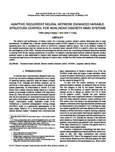
The optimal electromagnetic performance for the actuator is therefore realized by controlling the primary current distributions to lie in the q-axis, i.e., i d=0 and this will yield a linear force per amp characteristic for the actuator. The configuration of a field-oriented PMLSM servo drive system is shown in Fig. 1, where d is the position of the mover; d * is the position command; v * is the velocity command; i a* , i b* and i c* are the

30

Journal of the Chinese Institute of Engineers, Vol. 25, No. 1 (2002)

Fig. 1 System configuration of field-oriented PMLSM drive

three-phase command currents; i a and i b are the A and B phase currents; T a , T b and T c are the switching signals of the inverter. The drive system consists of a PMLSM, a ramp comparison current-controlled PWM VSI, a field-orientation mechanism, a coordinate translator, a speed control loop, a position control loop, a linear scale and Hall sensors. The flux position of the PM is detected by the output signals of the Hall sensors denoted U, V and W and the mover position signal d. Different sizes of iron disks can be mounted on the PMLSM mover to change the mass of the moving element. With the implementation of field-oriented control, the PMLSM drive system can be simplified to a control system block diagram as shown in Fig. 2, in which

F e = K F i q*

(12)

K F=3π P λ PM /2τ

(13)

H p (s) =

1 = b Ms + D s + a

(14)

where KF is the thrust coefficient; i q* is the command of thrust current; s is the a Laplace’s operator. The IP position controller shown in Fig. 2 will be discussed in the next section. Curve-fitting technique based on step response of the mover position is applied here to find the model of the drive system. For the convenience of the controller design, the position and speed signals in the

Fig. 2

Simplified control system block diagram with IP position controller

control loop are set at 1V=0.063662m and 1V= 0.063662m/sec. The resulting system parameters are: KF=20 N/A, a=42.246, b=7.974

M =1.97kg=0.1254 Nsec/V D =83.2245 kg/sec=5.2982 N/V

(15)

The “ - ” symbol represents the system parameter in the nominal condition. III. DESIGN OF IP POSITION CONTROLLER To match the requirements of high performance applications, the desired specifications of position step command tracking usually are no overshoot, no steady-state error and preset of rise time t re . A systematic design procedure for an IP position

31

C.H. Lin & F.J. Lin: Recurrent Neural Network Controlled Linear Synchronous Motor Drive System

controller capable of satisfying the above specifications has been introduced in (Lin, 1997). The closedloop drive system with an IP position controller is shown in Fig. 2. The transfer function of the mover position response to the command input is

d(s) d *(s)

= w(s) = 0

K d K IK Fb s + (a + K p K F b)s 2 + K I K F bs + K d K I K F b 3

∆ h h h = s + 1µ + s + 2µ + s + 3µ 1 2 3

(16)

According to Lin (1997), if the unknown parameters µ 1 , µ 2 , µ 3 , h 2 and h 3 are solved according to the prescribed specifications, the parameters of the controllers can be computed using the following relationships: K p=( µ 1 + µ 2 + µ 3−a)/(K Fb)

(17)

K I=( µ 1 µ 2 + µ 2µ 3 + µ 1 µ3 )/(K Fb)

(18)

K d=( µ 1 µ 2µ 3 )/(KI K Fb)

(19)

Moreover, under the same time-domain control specifications, the parameters of the IP controller depend only on the parameters of the drive system. Though desired command tracking response can be satisfied by an IP position controller in the nominal case, the performance of the drive system is sensitive to parameter variations and external disturbances in the system. To solve this problem, a RNN control system will be proposed in the following section. IV. RECURRENT NEURAL NETWORK 1. Description of RNN A simple three-layer RNN as shown in Fig. 3, which comprises an input (the i layer), a hidden (the j layer) and an output layer (the k layer), is proposed to implement the position controller. The signal propagation and the activation function in each layer is introduced as follows: (i) Input Layer: net i(N)=x i (N), O i(N)=f i(net i(N))=

1 , i=1, 2 1 + e – net i (N) (20)

where x i represents the ith input to the node of the input layer; N denotes the number of iterations; f i is the activation function, which is a sigmoidal function. The inputs of the RNN are the tracking er-

Fig. 3 Structure of RNN

ror em, which is the difference between the output of the reference model dm and the mover position d, and its derivative. (ii) Hidden Layer:

net j (N) = W j O j (N – 1) + Σ W ji O i (N) , i

O j (N) = f j (net j (N)) =

1 , j=1, 2, ..., Rj 1 + e – net j (N)

(21)

where W j are the recurrent weights for the units in the hidden layer; W ji are the connective weights between the input layer and the hidden layer; R j is the number of neurons in the hidden layer; f j is the activation function, which is also a sigmoidal function. (iii) Output Layer:

net k (N) = Σ W kj O j (N) , O k(N)=f k(net k(N))=net k, k=1 j

(22) where Wkj are the connective weights between the hidden layer and the output layer; f k is the activation function, which is set to be unit. The output of the RNN is the control signal. 2. On-Line Learning Algorithm To describe the on-line learning algorithm of the RNN, first the energy function E is defined as

E = 1 (d m – d)2 = 1 e 2m 2 2

(23)

32

Journal of the Chinese Institute of Engineers, Vol. 25, No. 1 (2002)

Then, the learning algorithm based on dynamic backpropagation (Ku and Lee, 1995) is described below. (iv) Output Layer: The error term to be propagated is given by

∂E ∂e m ∂d δ k = – ∂E = – ∂e ∂O k m ∂d ∂O k

(24)

and the connecting weight is updated by the amount

∂O k = η kj δ k O j ∆W kj = – η kj ∂E = – η kj ∂E ∂W kj ∂O k ∂W kj

(25)

where the factor η kj is the learning-rate parameter of the connecting weights between the output layer and the hidden layer. The connective weights between the hidden layer and the output layer are updated according to the following equation: W kj (N+1)=W kj (N)+∆W kj(N)

Fig. 4 RNN position control system

computation effort is required. To overcome this problem and to increase the on-line learning speed of the weights, the delta adaptation law proposed in (Lin and Wai, 1998; Lin et al., 1999) is adopted as follows:

δ k=e m+pe m

(31)

(26) where pe m denotes the derivative of the output error e m.

(v) Hidden Layer: The recurrent weight is updated by the amount

3. Convergence Analyses

∂O k ∂O j = η j δ k W kj P j (27) ∆W j = – η j ∂E = – η j ∂E ∂W j ∂O k ∂O j ∂W j where Pj(N)≡∂Oj(N)/∂W j and the factor ηj is the learning-rate parameter of the recurrent weights in the hidden layer. The recurrent weights of the hidden layer are updated according to the following equation:

In order to train the RNN effectively, the proposed varied learning rates, which guarantee convergence of the tracking error based on the analyses of a discrete-type Lyapunov function, are derived in the Appendix. V. RNN CONTROL SYSTEM

W j (N+1)=W j(N)+∆W j(N)

(28)

The connecting weight is updated by the amount

∂O k ∂O j = η ji δ k W kj Q ji ∆W ji = – η ji ∂E = – η ji ∂E ∂W ji ∂O k ∂O j ∂W ji (29) where Q ji(N)≡∂O j (N)/∂W ji and the factor η ji is the learning-rate parameter of the connecting weights between the hidden layer and the input layer. The connective weights between the input layer and the hidden layer are updated according to the following equation: W ji(N+1)=W ji(N)+∆W ji(N)

(30)

The exact calculation of the Jacobian of the system, ∂d/∂O k, cannot be done due to the unknown disturbances of the LSM drive system. Though the RNN identifier (Ku and Lee, 1995) can be implemented to calculate the Jacobian of the system, heavy

The configuration of the proposed RNN control system for the LSM drive is shown in Fig. 4, in which the reference model is selected according to the desired time-domain specifications. In the RNN, the units in the input, hidden and output layers are two, twenty and one neurons, respectively. The inputs of the RNN are e m and its derivative pe m; the output of the RNN is the thrust command current i q* (O k). Moreover, all the learning-rate parameters are updated at the same time. To obtain a favorable model-following characteristic, the transfer function of the drive system controlled by the IP position controller in the nominal case as follows is chosen as the reference model for periodic step input:

357911 s 3 + 294s 2 + 19206s + 357911

(32)

On the other hand, the reference model is set to be one when the input is a periodic sinusoidal command. The output of the reference model is the desired mover position dm and its derivative v m.

C.H. Lin & F.J. Lin: Recurrent Neural Network Controlled Linear Synchronous Motor Drive System

33

At the nominal condition, when the mover position of the LSM drive deviates from the output of the reference model, the thrust command current, i q* (O k ), will be automatically generated by the RNN controller. Moreover, when parameter uncertainties or external disturbances occur, the degradation of the tracking performance is significantly reduced by this error-driven mechanism. The effectiveness of the online training RNN based on the proposed delta adaptation law and varied learning rates will be demonstrated using some experimental results in the next section. VI. SIMULATED AND EXPERIMENTAL RESULTS Using the parameters listed in Eq. (15) and setting tre=0.1sec, the parameters of the IP controller can be solved using Eq. (17) through Eq. (19) as K p=1.047, KI =81.556, K d=18.7339

(33)

The sampling interval of the control processing in both the simulation and experimentation are both set at 0.5msec. 1. Simulation To investigate the effectiveness of the proposed controllers, two kinds of disturbances, variation of the mover mass and external force disturbance, are considered here. The following cases were tested in the simulation: Nominal case (M= M ) w=0 at the first cycle Case 1: Parameter variation case (M=4.5 M ) w=0 at the other cycles w=0 0≤t≤0.4sec Case 2: Time-varying load w=20N 0.4sec