Jen-Tzung Chien and Jung-Chun Chen. Department of Computer Science and Information Engineering. National Cheng Kung University, Tainan, Taiwan, ROC.
RECURSIVE BAYESIAN REGRESSION MODELING AND LEARNING Jen-Tzung Chien and Jung-Chun Chen Department of Computer Science and Information Engineering National Cheng Kung University, Tainan, Taiwan, ROC {chien, jcchen}@chien.csie.ncku.edu.tw ABSTRACT This paper presents a new Bayesian regression and learning algorithm for adaptive pattern classification. Our aim is to continuously update regression parameters to meet nonstationary environments for real-world applications. Here, a kernel regression model is used to represent twoclass data. The initial regression parameters are estimated by maximizing the likelihood of training data. To activate online learning, we properly express the randomness of regression parameters as a conjugate prior, which is a normal-gamma distribution. When new adaptation data are enrolled, we can accumulate sufficient statistics and come up with a new normal-gamma distribution as the posterior distribution. We therefore exploit a recursive Bayesian algorithm for online regression and learning. Regression parameters are incrementally adapted to the newest environments. Robustness of classification rule is assured using online regression parameters. In the experiments on face recognition, the proposed regression algorithm outperforms support vector machine and relevance vector machine for different numbers of adaptation data. Index Terms—Recursive Bayesian learning, kernel regression, incremental adaptation, support vector machine, pattern recognition 1. INTRODUCTION Due to the power of model generalization, support vector machine (SVM) [13] has been attracting many researchers working on the related issues. Continuing improvements in SVM have led into many successful applications in pattern recognition, e.g. information retrieval [10], speech recognition [11], and face recognition [7]. However, in real-world applications, such generalization is not sufficient to meet continuously changing environments. For example, face recognition performance is always degraded when the environmental conditions of illumination, facial expression, and pose angle are mismatch with those in training data. We should build adaptation/learning mechanism to overcome mismatch problem. Especially, in nonstationary environments, testing conditions are varied all the time. How to build online adaptation for SVM or other models becomes important for robust pattern recognition [4]. In this study, we are developing online adaptation algorithm from Bayesian learning viewpoint. In the literature,
1424407281/07/$20.00 ©2007 IEEE
Bayesian interpretation of SVM has been discussed in [5][6]. Bayesian support vector regression with an evidence framework was proposed to connect the relations to MacKay’s Bayesian framework [8]. Nevertheless, it was necessary to compute the integral in evidence framework. Some approximations were engaged so that no exact Bayesian explanation for SVM was available. Although SVM could be interpreted by Bayesian theory, these methods were not developed for Bayesian learning in presence of nonstationary environments. For these results, we present a new recursive Bayesian (RB) regression framework for general pattern classification. This framework can fulfill the spirit of SVM, namely maximization of margin and minimization of classification errors. Attractively, we adopt the conjugate prior distribution to express the perturbation of regression parameters. When adaptation data are collected, we can produce a posterior distribution, which belongs to the same distribution family as prior function [2]. This reproducible prior/posterior pair activates an online learning strategy for kernel regression model. This RB method can be also simplified as a batch learning that only one learning epoch is executed. We investigate the performance of online regression model on FERET facial database containing various conditions of lighting, expression and orientation. In what follows, we begin with a survey of regression models for pattern classification. Subsequently, we construct the recursive Bayesian approach to kernel regression model and explain its relations to previous methods. Finally, we demonstrate the performance of proposed method and draw some conclusions. 2. RELATED WORKS We are introducing Bayesian kernel regression methods. Some notations should be explained. Given input data x m , we transform it to high dimensional space z d , d ! m , using function M (x) . We collect a set of input-output training samples D {( z i , y i )}in 1 for supervised training. Kernel function is calculated by dot product of two samples K ( x i , x j ) M ( x i ) M (x j ) z i z j . Considering a two-class pattern classification problem, output y i represents class label, e.g. y i �1 for class 1 and y i �1 for class 2.
II 557
ICASSP 2007
2.1. Bayesian Support Vector Regression Using SVM, we are seeking the optimal hyperplane f (w , z ) w T z � b , which has the maximum margin between support vectors of two classes. Vapnik [13] also extended SVM to kernel-based support vector regression (SVR). In SVR, training samples of a class are represented by (1) yi wT z i � b � H � [i . This H insensitive loss function [13] was presented to obtain the sparseness property of SVM. Hence, we have [ i , [ i* y i � f (x i , w ) H as a modeling error with value of H being margin width. H is empirically defined. Using this loss function, the estimation accuracy of outliers will not hurt too much. The optimal parameters of w and b are obtained according to the least square error criterion 1 w 2
2
n
� C ¦ ([ i � [ i ) .
(2)
i 1
How to automatically determine regularization parameter C for various datasets becomes a crucial issue. Kwok [5] illustrated the relationship between SVM and MacKay’s Bayesian framework. The hyperparameters of SVM were estimated by maximizing the evidence. In SVR model [6], the parameter w was assumed to be random and C E D . Meaningfully, the hyperparameter D controls the model complexity. The hyperparameter E controls the training error. The prior distribution of w is Gaussian distributed p (w D ) v exp(�
D
2
2
w ).
(3)
Assuming training samples are i.i.d., the output distribution of training samples D is [5] n n p ( D w , E ) i 1 p( z i , y i w , E ) i 1 p( y i z i , w , E ) p ( z i ) , (4) where an exponential distribution is specified as p( y i z i , w, E )
E exp(� E [ i H ) 2(1 � HE )
.
The posterior probability of w can be formulated by p( D w, E ) p(w D ) . p ( w D, D , E ) ³ p( D w, E ) p(w D )dw
(5)
(6)
The optimal parameter of w is calculated by maximizing this posterior probability. Optimal MAP estimate w MAP is used to approximate the evidence in (6). Optimal values of D and E are then obtained by iterating the process of finding w MAP and maximizing the evidence. Parameter b is determined correspondingly. The integral in evidence is done in accordance with MacKay’s evidence framework [8]. In [1], SVR was regarded as a classification problem in the dual space. No model learning was concerned in these works. 2.2. Relevance Vector Machine Accordingly, Tipping [12] presented Bayesian learning via a relevance vector machine (RVM). Different from
Bayesian SVR [6], RVM assumed that parameters Į and E are random. The training samples are represented as n
¦ wi K (x j , x i ) � b � [ j .
yj
(7)
i 1
where the relevance is revealed by kernel function K (xi , x j ) . ~ [w T , b]T denote model parameters. A normal Let w ~. distribution with adjustable variance Į is assumed for w The gamma distribution over Į with hyperparameter OD is given by p (Į )
n
Gamma(D i OD ) .
(8)
i 0
~ is given as A zero-mean Gaussian prior distribution over w ~ Į) p (w
n
ȃ (b 0,D 0�1 ) ȃ ( wi 0,D i�1 ) .
(9)
i 1
The likelihood function of all the data conditional on unknown parameters is expressed by n/2 ª E ~ )T (y � ĭw ~ )º ½ ~ , E ) (E ) exp«� (y � ĭw p (y w (10) »¾ n/2 ® (2S ) ¯ ¬ 2 ¼¿ where ĭ [I (x1 ),�,I (x n )]T is the n u (n � 1) matrix and I (xi ) [ K (xi , x1 ),�, K (xi , x n ), 1]T . Parameter E is a precision
in density (10). The gamma distribution over E is also engaged in (11) p ( E ) Gamma(E O E ) . These priors were assumed to be non-informative. Using (6), ~ as (9) and (10), we obtain the posterior distribution over w a Gaussian distribution ~ y , Į, E ) p (w
Ȉ (2S )
�1 / 2 ( n �1) / 2
ª 1 ~ º½ T �1 ~ ®exp«� (w � ȝ) Ȉ (w � ȝ)» ¾ , (12) ¼¿ ¯ ¬ 2
where the mean vector is ȝ E ȈĭT y , the covariance matrix is Ȉ ( EĭT ĭ � ĮI) �1 , and I is the (n � 1) u (n � 1) identity matrix. We have the result of w MAP ȝ . Optimal Į and E are obtained by MacKay’s evidence framework [8]. Finally, we can classify a test pattern according to likelihood function of (10). 3. RECURSIVE BAYESIAN REGRESSION Basically, Bayesian SVR [5][6] provided Bayesian solution to SVM and extended SVM paradigm to deal with regression problem. Instead of merging support vectors, RVM [12] took relevance vectors into account and derive the predictive posterior distribution to activate Bayesian ~ and their learning. Prior densities of parameters w hyperparameters Į, E were defined. It was necessary to approximate the multivariate integral of evidence in MacKay’s framework [8]. In this study, we focus on developing Bayesian and incremental learning strategy for kernel regression model. Dummy variable is introduced in regression model so as to fit in with the maximum margin criterion adopted in SVM or SVR.
II 558
3.1. Regression Model Estimation To follow up the objective of maximum margin in SVM, the dummy variable ci {0, 1} is merged in regression model for each data pair [9]. This dummy label is used to describe the supervision of input pattern. Similar to SVR in (1), the training samples are now represented as (13) yi wT z i � b � ciH � [i , where H can be regarded as the margin between two classes. ~ [ w , b, H ]T and the The model parameters turn out to be w input pattern can be extended to ~zi [z Ti ,1, ci ]T . We can find ~ by the least-square solution to regression parameters w minimizing n
¦ ~
i 1
[ i2
~~ ~~ T ), ) ( y � Zw (y � Zw
T
ȟ ȟ
(14)
where Z [~z1 ,�, ~zn ]T . Reducing this expected error is able to achieve maximum margin and minimum classification ~ ~ error. The least-squares estimator is built by wˆ ZT ĭ �1y
from previous data sequence D t �1 {D (1) , � , D (t �1) } . We are calculating the posterior distribution, which combines the likelihood function of current block data D (t ) and the prior density calculated from historical data D t �1 ~ t , E Dt ) p(w
~ (t ) , w ~ t �1 , E y (t ) , y t �1 ) p(w
~ (t ) , E ) p (y t �1 w ~ t �1 , E ) p (w ~ (t ) , w ~ t �1 E ) p ( E ) v p ( y (t ) w �1 ª E ~ (t ) ½ ~ (t ) � w ˆ (t ) )T 1( d � 2 )un R (t ) 1n u( d � 2 ) (w ˆ (t ) )º» ¾ ®exp «� (w � w t t 2 ¬ ¼ ¯ ¿
ª u ®exp «� ¯ ¬ ª ° u ®exp «� °¯ «¬
E ~ t �1 ˆ t �1 )T 1 (w � w 2
( d � 2 )unt �1
½ ~ t �1 � w ˆ t �1 ) º» ¾ ( R t �1 ) �1 1nt �1u( d � 2 ) (w ¼¿
T ~ t �1 � w ˆ t �1 º E ªw
ª(R t �1 ) �1 V º 1( 2 d � 4 )unt « « ~ (t ) (t ) » T ( t ) �1 » ˆ ¼» 2 ¬« w � w V R ( ) ¼» ¬«
~ t �1 � w ªw ˆ t �1 º º ½° u 1nt u( 2 d � 4 ) « ~ (t ) »»¾ ˆ (t ) ¼» ¼» ° ¬« w � w ¿
where
~ ~ ~ ĭ [ĭ1 ,�, ĭ n ]T is a n u n matrix given ~ T ~ ~ ~ ~ ĭi [ zi z1 ,�, zi zn ] . We can rearrange (14) to be [9] ~~ T ~~ ~ T ~ ~ ~ ~ ~ ˆ ) ( y � Zw ˆ ) � [Z(w ˆ )]T [Z( w ˆ )] ( y � Zw ) ( y � Zw ) ( y � Zw �w �w
° ( t ) ª E º °½ ° t �1 ª E º ½° (18) u ®E J �1 exp «� (t ) » ¾ ®E J �1 exp «� t �1 » ¾ K °¯ ° ° ¬ ¼¿ ¯ ¬ K ¼ °¿ ~ ~ where V Zt �1 Z �t and nt nt �1 � nt . Hence, we have a
(15) After careful derivation and consideration of (10)(15) and the assumption in RVM, we write the likelihood function in a form of
posterior distribution such as this form
ª E ~ 1 ˆ ) T 1 ( d � 2)un R �1 exp «� ( w � w n/2 ® ( 2S ) ¯ ¬ 2
~ , E ,J ) p(y w
(16)
viewed as a gamma density for E . This distribution is known as normal-gamma distribution. 3.2. Recursive Bayesian for Incremental Learning To activate incremental learning, we select the prior ~ and E as a conjugate density of regression parameters w prior [3], which is a normal-gamma distribution ~ , E ) v Normal � Gamma( w ˆ , R , J ,K ) . (17) p (w Advantage of considering this conjugate prior is twofold. First, the prior density and the pooled posterior density belong to the same distribution family so that the incremental learning mechanism can be activated. Second, the computation of model parameters is efficient because the mode of posterior density turns out to be MAP estimate. In incremental learning, we collect a sequence of block data D T {D (1) , � , D (T ) } for model adaptation in individual epoch. At learning epoch t , we have current block data D (t ) {( z i(t ) , yi(t ) )}in 1 and sufficient statistics accumulated t
(19)
where ˆt w
ª E º½ ~ �w ˆ ) °® E J �1 exp «� » °¾ u 1 nu( d � 2) ( w °¯ ¬ K ¼ °¿ ~ �1 ~ T ~ -1 ˆ ) ( y � Zw ˆ ) and where R ĭ , J (n � 2) / 2 , K (y � Zw 1ij 1 for all i, j . In (16), the first term is viewed as a ~ given E , and the second term is Gaussian density for w
@`
~ t , E D t ) v Normal � Gamma(w ˆ t , R t , J t ,K t ) , p (w
ªw ˆ t �1 º t « (t ) » , R ˆ »¼ «¬ w
ª2( R t �1 ) �1 « T «¬ V
º » 2( R (t ) ) �1 »¼ V
�1
, Kt
K t �1K (t ) K t �1 � K (t )
and J t J t �1 � J (t ) . Attractively, the posterior distribution in (19) comes up with a normal-gamma distribution which is the same as the prior distribution determined from previous data D t �1 . It is important that the hyperparameters of new normal-gamma distribution provide the updating mechanism of sufficient statistics from (wˆ t �1 , R t �1 , J t �1 ,K t �1 ) to (wˆ t , R t , J t ,K t ) . Using this reproducible normal-gamma distribution, we are able to learn kernel regression parameters for any time when a block of adaptation data is enrolled. Different from SVR and RVM, we don’t need to apply evidence framework to find hyperparameters. The existing models can be adapted to the nonstationary environments. Robustness of pattern recognition is guaranteed. 4. EXPERIMENTS 4.1. Experimental Conditions In this paper, we evaluate the performance of recursive Bayesian regression for face recognition on public domain FERET database. We selected 200 persons from b set of FERET database. Each person had 11 face images. Resolution of each image was in 256 u 384 pixels. Face region was in 138 u 156 pixels. As shown in Figure 1, ba, bj and bk indicate the frontal images. bj and bk has different
II 559
facial expression and lighting condition, respectively. bb through bi is a series of images under different pose angles.
ba
bj
bk
bb bc bd be bf bg bh Bi Figure 1: Examples of one person in FERET database. To test system robustness, for each person, we adopted three images, ba, be, and bf, to train the initial prior model in (16)(17). Number of adaptation data for initial prior model was equivalent to 0. We performed five-fold cross validation through random selection from the other images. For each person, four images were selected for examination of batch learning as well as incremental learning. The remaining four images served as test images. Here, we used RBF kernel function K (x i , x j )
�2 exp®� V RBF xi � x j ¯
2½
¾. ¿
(20)
2 with the given parameter V RBF 100 . The regularization parameter C was obtained by Bayesian SVM method [5].
RBR RVM Batch SVM Incremental SVM
Recognition Accuracy (%)
90 89 88 87 86 85 84 0
1
2
3
Number of Adaptation Data
4
Figure 2: Comparison of recognition accuracies (%) using SVM, RVM and RBR. 4.2. Experimental Results In Figure 2, we compare the results of the proposed recursive Bayesian regression (RBR) algorithm, SVM and RVM. These methods are based on binary classification, one-against-one strategy. Class number is 200. Batch SVM [13], incremental SVM [4] and RVM [12] were carried out. The proposed RBR method achieves over 85% recognition accuracy. The accuracies of RBR method are better than batch SVM, incremental SVM and RVM. We do see the consistent improvement by increasing number of adaptation data. These results show a significant performance by adapting the facial kernel regression when testing on the data in different environments.
5. CONCLUSION We have presented a novel recursive Bayesian regression approach for online pattern recognition. Importantly, the relations to SVM, SVR and RVM were illustrated. The updating mechanism of sufficient statistics was developed. The advantages of proposed RVR method were its fast and robust capabilities. We have shown the improvement of face recognition compared to SVM and RVM. The incremental learning improvement from adaptation data was confirmed. The spirit of SVM with maximum margin and minimum error will be illustrated in the future. 6. REFERENCES [1] J. Bi and K. P. Bennett, “A geometric approach to support vector regression”, Neurocomputing, vol. 55, nos. 1-2, pp. 79-108, 2003. [2] J.-T. Chien, “Quasi-Bayes linear regression for sequential learning of hidden Markov models”, IEEE Transactions on Speech and Audio Processing, vol. 10, no. 5, pp. 268-278, 2002. [3] M. H. DeGroot, Optimal Statistical Decisions, McGraw-Hill, 1970. [4] C. P. Diehl and G. Cauwenberghs, “SVM incremental learning, adaptation and optimization”, in Proc. IEEE Int. Joint Conf. on Neural Networks, vol. 4, pp. 26852690, 2003. [5] J. T.-Y. Kwok, “The evidence framework applied to support vector machines”, IEEE Transactions on Neural Networks, vol. 11, no. 5, pp.1162-1173, 2000. [6] M. H. Law, J. T. Kwok, “Bayesian support vector regression”, in Proc. 8th Int. Workshop on Artificial Intelligence and Statistics, pp.239-244, 2001. [7] Z. Li and X. Tang, “Bayesian face recognition using support vector machine and face clustering”, in Proc. IEEE Int. Conf. Computer Vision and Pattern Recognition, vol. 2, pp. 374-380, 2004. [8] D. J. C. MacKay, “Bayesian interpolation”, Neural Computation, vol. 4, no. 3, pp. 415-447, 1992. [9] J. O. Rawlings, S. G. Pantula and D. A. Dickey, Applied Regression Analysis – A Research Tool, Springer-Verlag, Inc., 1998. [10] K. Shima, M. Todoriki and A. Suzuki, “SVM-based feature selection of latent semantic feature”, Pattern Recognition Letters, vol. 25, no. 9, pp. 1051-1057, 2004. [11] N. D. Smith and M. J. F. Gales, “Using SVMs and discriminative models for speech recognition”, in IEEE Proc. Int. Conf. Acoustics, Speech, Signal Processing, vol. 1, pp. 77-80, 2002. [12] M. E. Tipping, “Sparse Bayesian learning and the relevance vector machine”, Journal of Machine Learning Research, vol. 1, pp. 211-244, 2001. [13] V. N. Vapnik, Statistical Learning Theory, Wiley, 1998.
II 560