Bayesian Wavelet Regression on Curves With Application to a Spectroscopic Calibration Problem P. J. Brown, T. Fearn, and M. Vannucci Motivated by calibration problems in near-infrared (N IR) spectroscopy, we consider the linear regression setting in which the many predictor variables arise from sampling an essentially continuous curve at equally spaced points and there may be multiple predictands. We tackle this regression problem by calculating the wavelet transforms of the discretized curves, then applying a Bayesian variable selection method using mixture priors to the multivariate regression of predictands on wavelet coef cients. For prediction purposes, we average over a set of likely models. Applied to a particular problem in N IR spectroscopy, this approach was able to nd subsets of the wavelet coef cients with overall better predictive performance than the more usual approaches. In the application, the available predictors are measurements of the N IR re ectance spectrum of biscuit dough pieces at 256 equally spaced wavelengths. The aim is to predict the composition (i.e., the fat, our, sugar, and water content) of the dough pieces using the spectral variables. Thus we have a multivariate regression of four predictands on 256 predictors with quite high intercorrelation among the predictors. A training set of 39 samples is available to t this regression. Applying a wavelet transform replaces the 256 measurements on each spectrum with 256 wavelet coef cients that carry the same information. The variable selection method could use subsets of these coef cients that gave good predictions for all four compositional variables on a separate test set of samples. Selecting in the wavelet domain rather than from the original spectral variables is appealing in this application, because a single wavelet coef cient can carry information from a band of wavelengths in the original spectrum. This band can be narrow or wide, depending on the scale of the wavelet selected. KEY WORDS: Markov chain Monte Carlo; Mixture prior; Model averaging; Multivariate regression; Near-infrared spectroscopy; Variable selection.
1.
INTRODUCTION
This article presents a new way of tackling linear regression problems in which the predictor variables arise from sampling an essentially continuous curve at equally spaced points. The work was motivated by calibration problems in near-infrared (N IR) spectroscopy, of which the following example is typical. 1.1
Near-Infrared Spectroscopy of Biscuit Doughs
Quantitative N IR spectroscopy is used to analyze such diverse materials as food and drink, pharmaceutical products, and petrochemicals. The N IR spectrum of a sample of, say, wheat our is a continuous curve measured by modern scanning instruments at hundreds of equally spaced wavelengths. The information contained in this curve can be used to predict the chemical composition of the sample. The problem lies in extracting the relevant information from possibly thousands of overlapping peaks. Osborne, Fearn, and Hindle (1993) described applications in food analysis and reviewed some of the standard approaches to the calibration problem. The example studied in detail here arises from an experiment done to test the feasibility of N IR spectroscopy to P. J. Brown is P zer Professor of Medical Statistics, Institute of Mathematics and Statistics, University of Kent, Canterbury, Kent, CT2 7NF, U.K. (E-mail:
[email protected]). T. Fearn is Professor of Applied Statistics, Department of Statistical Science, University College London, WC1E 6BT, U.K. (E-mail:
[email protected]). M. Vannucci is Assistant Professor of Statistics, Department of Statistics, Texas A&M University, College Station, TX 77843 (E-mail:
[email protected]). This work was supported by the U.K. Engineering and Physical Sciences Research Council under the Stochastic Modelling in Science and Technology Initiative, grant GK/K73343. M. Vannucci also acknowledges support from the Texas Higher Advanced Research Program, grant 010366-0075 from Texas A&M International Research Travel Assistant Program and from the National Science Foundation CAREER award DMS-0093208. The spectroscopic calibration problem was provided by the Flour Milling and Baking Research Association. The authors thank the associate editor and a referee, as well as Mike West, Duke University, and Adrian Raftery, University of Washington, for suggestions that helped improve the article.
measure the composition of biscuit dough pieces (formed but unbaked biscuits), for possible on-line implementation. (For a full description of the experiment, see Osborne, Fearn, Miller, and Douglas 1984.) Brie y, two similar sample sets were made up, with the standard recipe varied to provide a large range for each of the four constituents under investigation: fat, sucrose, dry our, and water. The calculated percentages of these four ingredients represent the q D 4 responses. There were n D 39 samples in the calibration or training set, with sample 23 excluded from the original 40 as an outlier, and a further m D 39 in the separate prediction or validation set, again after one outlier was excluded. Thus Y and Yf , the matrices of compositional data for the training and validation sets, are both of dimension 39 4. An N IR re ectance spectrum is available for each dough piece. The original spectral data consist of 700 points measured from 1100 to 2498 nanometers (nm) in steps of 2 nm. For our analyses using wavelets, we have chosen to reduce the number of spectral points to save computational time. The rst 140 and last 49 wavelengths, which were thought to contain little useful information, were removed, leaving a wavelength range from 1380 nm to 2400 nm, over which we took every other point, thus increasing the gap to 4 nm and reducing the number of points to p D 256. The matrices X and Xf of spectral data are then 39 256. Samples of three centered spectra are given on the left side of Figure 1. The aim is to derive an equation that will predict the response values Y from the spectral data X for future samples where Y is unknown but X can be measured cheaply and rapidly.
398
© 2001 American Statistical Association Journal of the American Statistical Association June 2001, Vol. 96, No. 454, Applications and Case Studies
Brown, Fearn and Vannucci: Bayesian Wavelet Regression on Curves
399
– 0.08
0 DWT
0.5
Reflectance
– 0.06
– 0.1
– 0.5
– 0.12
–1
– 0.14 1400
1600
1800
2000
2200
– 1.5
2400
50
100
150
200
250
0
50
100
150
200
250
0
50
100 150 200 Wavelet coefficient
250
1
DWT
Reflectance
0.1
0
0.05
0 1400
1600
1800
2000
2200
0.5 0
– 0.5
2400
0.06
0.4 DWT
Reflectance
0.08
0.04 0.02
0.2 0
0 1400
1600
1800 2000 Wavelength
2200
– 0.2
2400
Figure 1. Original Spectra (left column) and Wavelet Transforms (right column).
1.2
Standard Analyses
The most commonly used approaches to this calibration problem regress Y on X, with the linear form Y D XB C E being justi ed either by appeals to the Beer–Lambert law (Osborne et al. 1993) or on the grounds that it works in practice. In Section 6 we also investigate logistic transformations of the responses, showing that overall their impact on the prediction performance of the model is not bene cial. The problem is not straightforward, because there are many more predictor variables (256) than training samples (39) in our example. The most commonly used methods for overcoming this dif culty fall into two broad classes: variable selection and factor-based methods. When scanning N IR instruments rst appeared, the standard approach was to select (typically using a stepwise procedure) predictors at a small number of wavelengths and use multiple linear regression with this subset (Hrushka 1987). Later, this approach was largely superseded by methods that reduce the p spectral variables to scores on a much smaller number of factors and then regress on these scores. Two variants—principal components regression (PCR; Cowe and McNicol 1985) and partial least squares regression (PLS; Wold, Martens, and Wold 1983)—are now widely used, with equal effectiveness, as the standard approaches. The increasing power of computers has triggered renewed research interest in wavelength selection, now using computer-intensive search methods.
1.3
Selecting Wavelet Coef’ cients
The approach that we investigate here involves selecting variables, but we select from derived variables. The idea is to transform each spectrum into a set of wavelet coef cients, the whole of which would suf ce to reconstruct the spectrum, and select good predictors from among these. There are good reasons for thinking that this approach might have advantages over selecting from the original variables. In previous work (Brown, Fearn, and Vannucci 1999; Brown, Vannucci, and Fearn 1998a,b) we explored Bayesian approaches to the problem of selecting predictor variables in this multivariate regression context. We apply this methodology to wavelet selection here. We know that wavelets can be used successfully for compression of curves like the spectra in our example, in the sense that the curves can be accurately reconstructed from a fraction of the full set of wavelet coef cients (Trygg and Wold 1998; Walczak and Massart 1997). Furthermore, the wavelet decomposition of the curve is a local one, so that if the information relevant to our prediction problem is contained in a particular part or parts of the curve, as it typically is, then this information will be carried by a very small number of wavelet coef cients. Thus we may expect selection to work. The ability of wavelets to model the curve at different levels of resolution gives us the option of selecting from our curve at a range of bandwidths. In some situations it may be advantageous to select a sharp band, as we do when we select one of the original variables; in other situations a broad band, averaging over many adjacent points, may be preferable. Selecting from the wavelet coef cients gives us both of these options automatically and in a very computationally ef cient framework.
400
Journal of the American Statistical Association, June 2001
Not surprisingly, Fourier analysis has also been successfully used for data compression and denoising of N IR spectral data (McClure, Hamid, Giesbrecht, and Weeks 1984). For this purpose, there is probably very little to choose between the Fourier and wavelet approaches. When it comes to selecting small numbers of coef cients for prediction, however, the local nature of wavelets makes them the obvious choice. It is worth emphasizing that what we are doing here is not what is commonly described as wavelet regression. We are not tting a smooth function to a single noisy curve by using either thresholding or shrinkage of wavelet coef cients (see Clyde and George 2000 for Bayesian approaches that use mixture modeling and Donoho, Johnstone, Kerkyacharian, and Picard 1995). Unlike those authors, we have several curves, the spectra of 39 dough pieces, each of which is transformed to wavelet coef cients. We then select some of these wavelet coef cients (the same ones for each spectrum), not because they give a good reconstruction of the curves (which they do not) or to remove noise (of which there is very little to start with) from the curves, but rather because the selected coef cients are useful for predicting some other quantity measured on the dough pieces. One consequence of this is that it is not necessarily the large wavelet coef cients that will be useful; small coef cients in critical regions of the spectrum also may carry important predictive information. Thus the standard thresholding or shrinkage approaches are just not relevant to this problem. 2. 2.1
PRELIMINARIES
Wavelet Bases and Wavelet Transforms
Wavelets are families of functions that can accurately describe other functions in a parsimonious way. In L2 425, for example, an orthonormal wavelet basis is obtained as translations and dilations of a mother wavelet – as –j1 k 4x5 D 2j=2 –42j x ƒ k5 with j1 k integers. A function f is then represented by a wavelet series as X f 4x5 D dj1 k –j1 k 4x51 (1)
the ne J ƒ 1 to a coarser one, say J ƒ r . An algorithm for the inverse construction also exists. Wavelet transforms can be computed very rapidly and have good compression properties. Because they are localized in both time and frequency, wavelets have the ability to represent many classes of functions in a sparse form by describing important features with few coef cients. (For a general exposition of wavelet theory see Daubechies 1992.) 2.2
Matrix-Variate Distributions
In what follows we use notation for matrix-variate distributions due to Dawid (1981). We write VƒM
® 4â 1 è5
when the random matrix V has a matrix-variate normal distribution with mean M and covariance matrices ƒii è and ‘ jj â for its ith row and jth column. Such a V could be generated as V D M C A0 UB, where M1 A1 and B are xed matrices such that A0 A D â and B0 B D è and U is a random matrix with independent standard normal entries. This notation has the advantage of preserving the matrix structure instead of reshaping V as a vector. It also makes for much easier formal Bayesian manipulation. The other notation that we use is W
© · 4„3 è5
for a random matrix W with an inverse Wishart distribution with scale matrix è and shape parameter „. The shape parameter differs from the more conventional degrees of freedom, again making for very easy Bayesian manipulations. With U and B de ned as earlier, and with U as n p with n > p, W D B0 4U0 U5ƒ1 B has an inverse Wishart distribution with shape parameter „ D n ƒ p C 1 and scale matrix è. The expectation of W exists for „ > 2 and is then è=4„ ƒ 25. (More details of these notations, and a corresponding form for the matrix-variate T , can be found in Brown 1993, App. A, or Dawid 1981.)
j1 k2:
R with wavelet coef cients dj1 k D f 4x5–j1 k 4x5dx describing features of the function f at the spatial location 2ƒj k and frequency proportional to 2j (or scale j). Daubechies (1992) proposed a class of wavelet families that have compact support and a maximum number of vanishing moments for any given smoothness. These are used extensively in statistical applications. Wavelets have been an extremely useful tool for the analysis and synthesis of discrete data. Let Y D 4y1 1 : : : 1 yn 5, n D 2J , be a sample of a function at equally spaced points. This vector of observations can be viewed as an approximation to the function at the ne scale J . A fast algorithm, the discrete wavelet transform (DWT), exists for decomposing Y into a set of wavelet coef cients (Mallat 1989) in only O4n5 operations. The DWT operates in practice by means of linear recursive lters. For illustration purposes, we can write it in matrix form as Z D WY, where W is an orthogonal matrix corresponding to the discrete wavelet transform and Z is a vector of wavelet coef cients describing features of the function at scales from
3. 3.1
MODELING
Multivariate Regression Model
The basic setup that we consider is a multivariate linear regression model, with n observations on a q-variate response and p explanatory variables. Let Y denote the n q matrix of observed values of the responses and let X be the n p matrix of predictor variables. Our special concern is with functional predictor data; that is, the situation in which each row of X is a vector of observations of a curve x4t5 at p equally spaced points. The standard multivariate normal regression model has, conditional on 1 B1 è, and X, 0 Y ƒ 1n ƒ XB
® 4 In 1 è51
(2)
where 1n is an n 1 vector of 1’s, is a q 1 vector of intercepts, and B D 4‚1 1 : : : 1 ‚q 5 is a p q matrix of regression coef cients. Without loss of generality, we assume that the columns of X have been centered by subtracting their means.
Brown, Fearn and Vannucci: Bayesian Wavelet Regression on Curves
The unknown parameters are , B, and the q q error covariance matrix è. A conjugate prior for this model is as follows. First, given è, 0 ƒ 00
® 4h1 è5
(3)
B ƒ B0
® 4H1 è50
(4)
and, independently,
The marginal distribution of è is then è
© · 4„3 Q50
(5)
Note that the priors on both and B have covariances dependent on è in a way that directly extends the univariate regression natural conjugate prior distributions. In practice, we let h ! ˆ to represent vague prior knowledge about and take B0 D 0, leaving the speci cation of H, „, and Q to incorporate prior knowledge about our particular application. 3.2
Transformation to Wavelets
We now transform the predictor variables by applying to each row of X a wavelet transform, as described in Section 2.1. In matrix form, multiplying each row of X by the same matrix W is equivalent to multiplying X on the right side by W0 . The wavelet transform is orthogonal (i.e., W0 W D I), and thus (2) can be written as Y ƒ 1n 0 ƒ XW 0 WB
® 4 In 1 è50
(6)
We can now express the model in terms of wavelet transformations of the predictors as 0 Q Y ƒ 1n ƒ Z B
® 4 In 1 è51
(7)
where Z D XW 0 is now a matrix of wavelet coef cients and Q D WB is a matrix of regression coef cients. The transB Q in the case of inclusion of all predictors, is formed prior on B, BQ
Q è51 ® 4H1
401
3.3
To perform selection in the wavelet coef cient domain, we Q by introducing a latent binary further elaborate the prior on B p-vector ƒ. The jth element of ƒ1 ƒj , may be either 1 or 0, depending on whether the jth column of Z is or is not included in the model. When ƒj is unity, the covariance matrix Q is “large,” and when ƒ is 0, the of the corresponding row of B j covariance matrix is a zero matrix. We have assumed that the Q is 0, and so ƒ D 0 effectively deletes prior expectation of B j the jth explanatory variable (or wavelet coef cient) from the model. This gives, conditional on ƒ, BQ ƒ
Q 1 è51 ® 4H ƒ
(9)
Q and H Q are just BQ and H Q with the rows and, in where B ƒ ƒ Q the case of H, columns for which ƒj D 0 deleted. Under this prior, each row of BQ is modeled as having a scale mixture of the type Q 6 B7 6j27
41 ƒ ƒj 5I0 C ƒj N 401 hQ jj è51
(10)
Q D with hQ jj equal to the jth diagonal element of the matrix H 0 WHW and I0 a distribution placing unit mass on the 1 q Q are not independent. zero vector. Note that the rows of B A simple prior distribution 4ƒ5 for ƒ takes the ƒj to be independent with Pr4ƒj D 15 D wj and Pr4ƒj D 05 D 1 ƒ wj , with hyperparameters wj to be speci ed, for j D 11 : : : 1 p. In our example we take all of the wj equal to a common w, so that the nonzero elements of ƒ have a binomial distribution with expectation pw. Mixture priors have been widely used for variable selection in the original model space, originally by Leamer (1978) and more recently by George and McCulloch (1997) and Mitchell and Beauchamp (1988) for the linear multiple regression case. Carlin and Chib (1995), Chipman (1996), and Geweke (1996), among others, concentrated on special features of these priors. Clyde, DeSimone, and Parmigiani (1996) used model mixing in prediction problems with correlated predictors when expressing the space of models in terms of an orthogonalization of the design matrix. Their methods are not directly applicable to our situation, because the wavelet transforms do not leave us with an orthogonal design. The use of mixture priors for selection in the multivariate regression setup has been investigated by Brown et al. (1998a,b). 4.
(8)
Q D WHW0 and the parameters and è are unchanged where H by the orthogonal transformations, as are the priors (3) and (5). In practice, wavelets exploit the recursive application of lters, and the W-matrix notation is more useful for explanation than for computation. Vannucci and Corradi (1999) proposed a fast recursive algorithm for computing quantities such as WHW0 . Their algorithm has a useful link to the twodimensional DWT (DWT2), making computations simple. The matrix WHW0 can be computed from H with an O4n2 5 algorithm. (For more details, see secs. 3.1 and 3.2 of Vannucci and Corradi 1999.)
A Framework for Variable Selection
4.1
SELECTING WAVELET COEFFICIENTS
Posterior Distribution of ƒ
The posterior distribution of ƒ given the data, 4ƒ — Y1 Z5, assigns a posterior probability to each ƒ-vector and thus to each possible subset of predictors (wavelet coef cients). This posterior arises from the combination of a likelihood that gives great weight to subsets explaining a high proportion of the variation in the responses Y and a prior for ƒ that penalizes large subsets. It can be computed by integrating out 1 B1 and è from the joint posterior distribution of these parameters and ƒ given the data. With the vague (h ! ˆ) prior for , this parameter is essentially estimated by the mean Y in the calibration data (see Smith 1973), and to simplify the formulas
402
Journal of the American Statistical Association, June 2001
that follow, we now assume that the columns of Y have been centered. (Full details of the prior to posterior analysis have been given by Brown et al. 1998b, who also considered other prior structures.) After some manipulation, we have 4ƒ — Y1 Z5 / g4ƒ5 D
Q Z0 Z C H Q ƒ1 H ƒ ƒ ƒ ƒ Qƒ
ƒq=2
ƒ4nC„Cqƒ15=2
1
Q ƒ2 Zƒ H ZQ ƒ D Ipƒ
´
1
4ƒ51
(11)
Q D Y 1 Y 0
Q 1=2 is a matrix square root of H Q and p is the number where H ƒ ƒ ƒ of 1’s in ƒ, the relevant quantities entering into (11) can be computed as Q Z0 Z C H Q ƒ1 D ZQ 0 Z Q H ƒ ƒ ƒ ƒ ƒ ƒ
(12)
Q 0Y Q ƒY Q 0Z Q 4ZQ 0 Z Q ƒ1 Q 0 Q Qƒ D Q C Y ƒ ƒ ƒ 5 Zƒ Y3
(13)
and
that is, Qƒ is given by Q plus the residual sum of prodQ on ZQ . ucts matrix from the least squares regression of Y ƒ The QR decomposition can then be used (see, e.g., Seber 1984, chap. 10, sec. 1.1b), which avoids “squaring” as in (12) and (13). 4.2
The new candidate model, ƒ ü , is accepted with probability min
Q ƒ1 5ƒ1 Z0 Y and Z is where Qƒ D Q C Y0 Y ƒ Y 0 Zƒ 4Z0 ƒ Zƒ C H ƒ ƒ ƒ Z with the columns for which ƒj D 0 deleted. Care is needed in computing (11); the alternative forms discussed later may be useful. A simplifying feature of this setup is that all of the computations can be formulated as least squares problems with modi ed Y and Z matrices. By writing
³
¡ Swap two components by choosing independently at random a 0 and a 1 in the current ƒ and changing both of them. This move is chosen with probability 1 ƒ ”.
Metropolis Search
Equation (11) gives the posterior probability of each of the 2p different ƒ vectors, and thus of each choice of wavelet coef cient subsets. What remains to do is to look for “good” wavelet components by computing these posterior probabilities. When p is much greater than about 25, too many subsets exist for this to be feasible. Fortunately, we can use simulation methods that will nd the ƒ vectors with relatively high posterior probabilities. We can then quickly identify useful coef cients that have high marginal probabilities of ƒj D 1. Here we use a Metropolis search, as suggested for model selection by Madigan and York (1995) and applied to variable selection for regression by Brown et al. (1998a), George and McCulloch (1997), and Raftery, Madigan, and Hoeting (1997). The search starts from a randomly chosen ƒ 0 and then moves through a sequence of further values of ƒ. At each step, the algorithm generates a new candidate ƒ by randomly modifying the current one. Two types of moves are used: ¡ Add or delete a component by choosing at random one component in the current ƒ and changing its value. This move is chosen with probability ”.
g4ƒ ü 5 11 0 g4ƒ5
(14)
Thus a more probable ƒ ü is always accepted, and a less probable one may be accepted. There is scope for further ingenuity in designing the sequence of random moves. For example, moves that add or subtract or swap two or three or more at a time, or a combination of these, may be useful. The sequence of ƒ’s generated by the search is a realization of a Markov chain, and the choice of acceptance probabilities ensures that the equilibrium distribution of this chain is the distribution given by (11). In typical uses of such schemes, the realizations are monitored after a suitable burn-in period to verify that they appear stationary. Here we have a closed form for the posterior distribution, and are using the chain simply to explore this distribution. Thus we have not been so concerned about strict convergence of the Markov chain. Following Brown et al. (1998a), we adopt a strategy of running the chain from a number of different starting points (four here) and looking at the four marginal distributions provided by the computed g4¢5 values of the visited ƒ’s. We also look for good indication of mixing and explorations with returns. Because we know the relative probabilities, we do not need to worry about using a burn-in period. Note that, given the form of the acceptance probability (14), ƒ-vectors with high posterior probability have a greater chance of appearing in the sequence. Thus we might expect that a long run of such a chain would visit many of the best subsets. 5.
PREDICTION
Suppose now that we wish to predict Yf , an m q matrix of further Y-vectors given the corresponding X-vectors, Xf 1 4m p5. First, we treat Xf exactly as the training data have been treated, by subtracting the training data means and transforming to wavelet coef cients Zf 1 4m p5. The model for Yf , following the model for the training data (6), is Yf ƒ 1m 0 ƒ Zf BQ
® 4 Im 1 è50
(15)
If we believe our Bayesian mixture model, then logically we should apply the same latent structure model to prediction as well as to training. This has the practical appeal of providing averaging over a range of likely models (Madigan and Raftery 1994). Results of Brown et al. (1998b) demonstrate that with the columns of Yf centered using the mean Y from the training set, the expectation of the predictive distribution p4Yf — O with ƒ1 Z1 Y5 is given by Zf B ƒ ƒ1
Q ƒ1 BO ƒ D Z0ƒ Zƒ C H ƒ
1
Q ƒ2 Z Q0 Z Q Z0ƒ Y D H ƒ ƒ
ƒ1
Q 0 Y0 Q Z ƒ
Averaging over the posterior distribution of ƒ gives O D XZ B O — Y f f ƒ 4ƒ Z1 Y51 ƒ
(16)
(17)
Brown, Fearn and Vannucci: Bayesian Wavelet Regression on Curves
403
and we might choose to approximate this by some restricted set of ƒ values, perhaps the r most likely values from the Metropolis search.
for each of the PCR equations. The results given in rows three and four of Table 1 show that, as usual, there is little to choose between the two methods. These results are for PLS and PCR using the reduced 256-point spectrum that we used for our wavelet analysis. Repeating the analyses using the original 700-point spectrum yielded results very similar to those for PLS and somewhat worse than those reported for PCR. Because shortly we need to specify a prior distribution on regression coef cients, it is interesting to examine those resulting from a factor-type approach. Combining the coef cients for the regression of constituent on factor scores with the loadings that produce scores from the original spectral variables gives the coef cient vector that would be applied to a measured spectrum to give a prediction. Figure 2 plots these vectors for the PLS equations for the four constituents, showing the smoothness in the 256 coef cients that we attempt to re ect in our prior distribution for B.
6. APPLICATION TO NEAR-INFRARED SPECTROSCOPY OF BISCUIT DOUGHS We now apply the methodology developed earlier to the spectroscopic calibration problem described in Section 1.1. First, however, we report the results of some other analyses of these data. 6.1
Analysis by Standard Methods
For all of the analyses carried out here, both compositional and spectral data were centered by subtracting the training set means from the training and validation data. The responses, but not the spectral data, were also scaled, to give each of the four variables unit variance in the training set. Mean squared prediction errors were converted back to the original scale by multiplying them by the training sample variances. This preprocessing of the data makes no difference to the standard analyses, which treat the response variables separately, but it simpli es the prior speci cation for our multivariate wavelet analysis. Osborne et al. (1984) derived calibrations by multiple regression, using various stepwise procedures to select wavelengths for each constituent separately. The mean squared error of predictions on the 39 validation samples for their calibrations are reported in the rst row of Table 1. Brown et al. (1999) also selected small numbers of wavelengths to nd calibration equations for this example. Their Bayesian decision theory approach differed from the approach of Osborne in being multivariate (i.e., in trying to nd one small subset of wavelengths suitable for predicting all four constituents) and in using a more extensive search using simulated annealing. The results for this alternative wavelength selection approach are given in the second row of Table 1. For the purpose of comparison, we carried out two other analyses using partial least squares regression (PLS) and principal components regression (PCR). These approaches, both of which construct factors from the full spectral data and then regress constituents on the factors, are very much the standard tools in N IR spectroscopy (see, e.g. Geladi and Martens 1996; Geladi, Martens, Hadjiiski, and Hopke 1996). For the computations, we used the PLS Toolbox 2.0 of Wise and Gallagher (Eigenvector Research, Manson, WA). Although there are multivariate versions of PLS, we took the usual approach of calibrating for each constituent separately. The number of factors used, selected in each case by cross-validation on the training set, was ve for each of the PLS equations and six Table 1. Mean Squared Errors of Prediction on the 39 Biscuit Dough Pieces in the Validation Set Using Four Calibration Methods Method
Fat
Sugar
Flour
Water
Stepwise MLR Decision theory PLS PCR
0044 0076 0151 0160
10188 0566 0583 0614
0722 0265 0375 0388
0221 0176 0105 0106
6.2
Wavelet Transforms of Spectra
To each spectrum we apply a wavelet transform, converting it to a set of 256 wavelet coef cients. We used the MATLAB toolbox Wavbox 4.3 (Taswell 1995) for this step. Using spectra with 2m (m integer) points is not a real restriction here. Methods exist to overcome the limitation, allowing the DWT to be applied on any length of data. We used MP(4) (Daubechies 1992, p. 194), wavelets with four vanishing moments. The Daubechies wavelets have compact support, important for good localization, and a maximum number of vanishing moments for a given smoothness. A large number of vanishing moments leads to high compressibility, because the ne-scale wavelet coef cients are essentially 0 where the functions are smooth. On the other hand, support of the wavelets increases with an increasing number of vanishing moments, so there is a trade-off with the localization properties. Some rather limited exploration suggested that the chosen wavelet family is a good compromise for these data. The graphs on the right side of Figure 1 show the wavelet transforms corresponding to the three N IR spectra in the left column. Coef cients are ordered from coarsest to nest. 6.3
Prior Settings
We need to specify the values of H, „, and Q in (3), (4), and (5) and the prior probability w that an element of ƒ is 1. We wish to put in weak but proper prior information about è. We choose „ D 3, because this is the smallest integer value such that the expectation of è, E4è5 D Q=4„ ƒ 25, exists. The scale matrix Q is chosen as Q D k Iq with k D 005, comparable in size to the expected error variances of the standardized Y given X. With „ small, the choice of Q is unlikely to be critical. Much more likely to be in uential are the choices of H and w in the priors for B and ƒ. To re ect the smoothness in the coef cients B, as exempli ed in Figure 2, while keeping the form of H simple, we have taken H to be the variance matrix of a rst-order autoregressive process, with hij D ‘ 2 —iƒj— . We derived the values ‘ 2 D 254 and D 032 by maximizing a type II likelihood (Good 1965). Integrating , B, and è from the joint distribution given by (2), (3), (4), and (5) for the
404
Journal of the American Statistical Association, June 2001
Coefficient
Fat
Sugar
6
4
4
2
2
0
0
–2
–2 1400
1600
1800
2000
2200
–4 1400
2400
1600
Flour
2000
2200
2400
2200
2400
Water
4
6 4
2 Coefficient
1800
2 0 0 –2
–4 1400
–2
1600
1800 2000 Wavelength
2200
–4 1400
2400
1600
1800 2000 Wavelength
Figure 2. Coef’ cient Vectors From 5-Factor PLS Equations.
regression on the full untransformed spectra, with h ! ˆ and B0 D 0, we get 0 f / —K—ƒq=2 —Q—4„Cqƒ15=2 —Q C Y Kƒ1 Y—ƒ4„CnCqƒ15=2 1
(18)
where K D In C XHX
0
and the columns of Y are centered, as in Section 4.1. With k D 005 and „ D 3 already xed, (18) is a function, via H, of ‘ 2 and . We used for our prior the values of these hyperparameters that maximize (18). Possible underestimation due to the use of the full spectra was taken into account by multiplying the estimate of ‘ 2 by the in ation factor 256=20, re ecting our prior belief as to the expected number of included coef cients. Q D Figure 3 shows the diagonal elements of the matrix H WHW0 implied by our choice of H. The variance matrix of the Q so this plot shows the pattern ith column of BQ in (8) is ‘ ii H, in the prior variances of the regression coef cients when the predictors are wavelet coef cients. The wavelet coef cients are ordered from coarsest to nest, so the decreasing prior variance means that there will be more shrinkage at the ner levels. This is a logical consequence of the smoothness that we have tried to express in the prior distribution. The spikes in the plot at the level transitions are from the boundary condition problems of the discrete wavelet transform. We know from experience that good predictions can usually be obtained with 10 or so selected spectral points in examples of this type. Having no previous experience in selecting
wavelet coef cients, and wanting to induce a similarly “small” model without constraining the possibilities too severely, we chose w in the prior for ƒ so that the expected model size was pw D 20. We have given equal prior probability here to coef cients at the different levels. Although we considered the possibility of varying w in blocks, we had no strong prior opinions about which levels were likely to provide the most useful coef cients, apart from a suspicion that neither the coarsest nor the nest levels would feature strongly. 6.4
Implementing the Metropolis Search
We chose widely different starting points for the four Metropolis chains, by setting to 1 the rst 1, the rst 20, the rst 128 (i.e., half), and all elements of ƒ. There were 100,000 iterations in each run, where an iteration comprised either adding/deleting or swapping, as described in Section 4.2. The two moves were chosen with equal probability ” D 1=2. Acceptance of the possible move by (14) was by generation of a Bernoulli random variable. Computation of g4ƒ5 and g4ƒ ü 5 was done using the QR decomposition of MATLAB. For each chain, we recorded the visited ƒ’s and their corresponding relative probability g4ƒ5. No burn-in was necessary, as relatively unlikely ƒ’s would automatically be downweighted in our analysis. There were approximately 38,000– 40,000 successful moves for each of the four runs. Of these moves, around 95% were swaps. The relative probabilities of the set of distinct visited ƒ were then normalized to 1 over this set. Figure 4 plots the marginal probabilities for components of ƒ1 P 4ƒj D 151 j D 11 : : : 1 256. The spikes show where regressor variables have been included in subsets with
Brown, Fearn and Vannucci: Bayesian Wavelet Regression on Curves
405
500
Prior variance of regression coefficient
450
400
350
300
250
200
150
0
50
100 150 Wavelet coefficient
200
250
Q D WHW 0 , With hQ Plotted Against i . Figure 3. Diagonal Elements of H ii
(i)
Probability
1 0.8
0.8
0.6
0.6
0.4
0.4
0.2
0.2
0
0
50
100
(ii)
1
150
200
250
0
0
50
Probability
(iii) 1
0.8
0.8
0.6
0.6
0.4
0.4
0.2
0.2
0
50
100 150 200 Wavelet coefficient
Figure 4.
150
200
250
100 150 200 Wavelet coefficient
250
(iv)
1
0
100
250
0
0
50
Marginal Probabilities of Components of ƒ for Four Runs.
406
Journal of the American Statistical Association, June 2001 (a)
Number of ones
120 100 80 60 40 20 0
0
1
2
3
4
5 6 Iteration number
7
8
9
10 4
x 10
(b)
0
Log probs
– 100
– 200
– 300
– 400 0
Figure 5.
1
2
3
4
5 6 Iteration number
8
9
10 4
x 10
Plots in Sequence Order for Run (iii). (a) The number of 1’s; (b) log relative probabilities.
high probability. For one of the runs, (iii), Figure 5 gives two more plots: the number of 1’s, and the log-relative probabilities, log4g4ƒ55, of the visited ƒ, plotted over the 100,000 iterations. The other runs produced very similar plots, quickly moving toward models of similar dimensions and posterior probability values. Despite the very different starting points, the regions explored by the four chains have clear similarities in that plots of marginals are overall broadly similar. However, there are also clear differences, with some chains making frequent use of variables not picked up by others. Although we would not claim convergence, all four chains arrive at some similarly “good,” albeit different, subsets. With mutually correlated predictor variables, as we have here, there will always tend to be many solutions to the problem of nding the best predictors. We adopt the pragmatic stance that all we are trying to do is identify some of the good solutions. If we happen to miss some other good ones, then this is unfortunate but not disastrous. 6.5
7
Results
We pooled the distinct ƒ’s visited by the four chains, normalized the relative probabilities, and ordered them according to probability. Then we predicted the further 39 unseen samples using Bayes model averaging. Mean squared prediction errors converted to the original scale were 00631 04491 0348, and 0050. These results use the best 500 models, accounting for almost 99% of the total visited probability and using 219 wavelet coef cients. They improve considerably on all of the standard methods reported in Table 1. The single best subset
among the visited ones had 10 coef cients, accounted for 9% of the total visited probability, and least squares predictions gave mean squared errors of 0059, 0466, 0351 and 0047. Examining the scales of the selected coef cients is interesting. The model making the best predictions used coef cients (10, 11, 14, 17, 33, 34, 82, 132, 166, 255), which include (0%, 0%, 0%, 37%, 6%, 6%, 1%, 2%) of all of the coef cients at the eight levels from the coarsest to the nest scales. The most useful coef cients seem to be in the middle of the scale, with some more toward the ner end. Note that the very coarsest coef cients, which would be essential to any reconstruction of the spectra, are not used, despite the smoothness implicit in H and the consequent increased shrinkage associated with ner scales, as seen in Figure 3. Some idea of the locations of the wavelet coef cients selected by the modal model can be obtained from Figure 6. Here we used the linearity of the wavelet transform and the linearity of the prediction equation to express the prediction equation as a vector of coef cients to be applied to the original spectral data. This vector is obtained by applying the inverse wavelet transform to the columns of the matrix of the least squares estimates of the regression coef cients. Because selection has discarded unnecessary details, most of the coef cients are very close to 0. We thus display only the 1600–1800 nm range, which permits a better view of the features of coef cients in the range of interest. These coef cient vectors can be compared directly with those shown in Figure 2. They are applied to the same spectral data to produce predictions, and despite the different scales, some comparisons are possible. For example, the two coef cient vectors for fat can be eas-
Brown, Fearn and Vannucci: Bayesian Wavelet Regression on Curves
407
ily interpreted. Fats and oils have absorption bands at around 1730 and 1765 nm (Osborne et al. 1993), and strong positive coef cients in this region are the major features of both plots. The wavelet-based equation (Fig. 6) is simpler, the selection having discarded much unnecessary detail. The other coef cient vectors show less resemblance and are also harder to interpret. One thing to bear in mind in interpreting these plots is that the four constituents add up to 100%. Thus it should not be surprising to nd the fat measurement peak in all eight plots nor that the coef cient vectors for sugar and our are so strongly inversely related. Finally, we comment brie y on results that we obtained by investigating logistic transformations of the data. Our response variables are in fact percentages and are constrained to sum up to 100; thus they lie on a simplex, rather than in the full q-dimensional space. Sample ranges are 18 3 for fat, 17 7 for sugar, 51 6 for our, and 14 3 for water. Following Aitchison (1986), we transformed the original Y 0 s into log ratios of the form
ing points used previously with the data in the original scale. Diagnostic plots and plots of the marginals appeared very similar to those of Figures 4 and 5. The four chains visited 151,183 distinct models. We nally computed Bayes model averaging and least squares predictions with the best model, unscaling the predicted values and transforming them back to the original scale as
Z1 D ln4Y1 =Y3 51
Z2 D ln4Y2 =Y3 51
and
Z3 D ln4Y4 =Y3 50
(19)
The choice of the third ingredient for the denominator was the most natural, in that our is the major constituent and also because ingredients in recipes often are expressed as a ratio to our content. We centered and scaled the Z variables and recomputed empirical Bayes estimates for ‘ 2 and . (The other hyperparameters were not affected by the logistic transformation.) We then ran four Metropolis chains using the start-
Y3 D P3
100 exp4Zi 5 Yi D P3 1 C1 jD1 exp4Zj 5
100
C1 jD1 exp4Zj 5
Fat
200
0
0
– 100
– 200
Coefficient
100
1600
1700
1800
– 400 1400
1500
Flour
200
100
0
0
– 200
– 100
Coefficient
200
1500
1600 Wavelength
1600
1700
1800
1700
1800
Water
400
– 400 1400
100 exp4Z3 5 Y4 D P3 0 C1 jD1 exp4Zj 5
Sugar 400
1500
and
The best 500 visited models accounted for 99.4% of the total visited probability, used 214 wavelet coef cients, and gave Bayes mean squared prediction errors of 0058, 0819, 0457, and 0080. The single best subset among the visited ones had 10 coef cients, accounted for 15.8% of the total visited probability, and gave least squares prediction errors of 00911 07931 0496, and 0119. The logistic transformation does not seem to have a positive impact on the predictive performance, and overall, the simpler linear model seems to be adequate. Our approach gives Bayes predictions on the original scale satisfying the constraint of summing exactly to 100. This stems from the conjugate prior, linearity in Y 1 zero mean for the prior distribution of the regression coef cients, and vague prior for the intercept. It is easily seen that with X centered, O 0 1 D 100 and BO 0 1 D 0 for either least squares or Bayes estimates, and hence all predictions sum to 100. In addition, had we imposed a singular distribution to deal with the four responses summing
200
– 200 1400
1
i D 11 21
1700
1800
– 200 1400
1500
1600 Wavelength
Figure 6. Coef’ cient Vectors From the “Best” Wavelet Equations.
408
Journal of the American Statistical Association, June 2001
to 100, then a proper analysis would suggest eliminating one component, but then the predictions for the remaining three components would be as we have derived. Thus our analysis is Bayes for the singular problem, even though super cially it ignores this aspect. This does not address the positivity constraint, but the composition variables are all so far from the boundaries compared to residual error that this is not an issue. Our desire to stick with the original scale is supported by the Beer–Lambert law, which linearly relates absorbance to composition. The logistic transform distorts this linear relationship. 7.
DISCUSSION
In specifying the prior parameters for our example, we made a number of arbitrary choices. In particular, the choice of H as the variance matrix of an autoregressive process is a rather crude representation of the smoothness in the coef cients. It might be interesting to try to model this in more detail. However, although there may be room for improvement, the simple structure used here does appear to work well. Another area for future investigation is the use of more sophisticated wavelet systems in this context. The additional exibility of wavelet packets (Coifman, Meyer, and Wickerhauser 1992) or m-band wavelets (Mallet, Coomans, Kautsky, and De Vel 1997) might lead to improved predictions, or might be just an unnecessary complication. [Received October 1998. Revised November 2000.]
REFERENCES Aitchison, J. (1986), The Statistical Analysis of Compositional Data, London: Chapman and Hall. Brown, P. J. (1993), Measurement, Regression, and Calibration, Oxford, U.K.: Clarendon Press. Brown, P. J., Fearn, T., and Vannucci, M. (1999), “The Choice of Variables in Multivariate Regression: A Bayesian Non-Conjugate Decision Theory Approach,” Biometrika, 86, 635–648. Brown, P. J., Vannucci, M., and Fearn, T. (1998a), “Bayesian Wavelength Selection in Multicomponent Analysis,” Journal of Chemometrics, 12, 173–182. , (1998b), “Multivariate Bayesian Variable Selection and Prediction,” Journal of the Royal Statistical Society, Ser. B, 60, 627–641. Carlin, B. P., and Chib, S. (1995), “Bayesian Model Choice via Markov Chain Monte Carlo,” Journal of the Royal Statistical Society, Ser. B, 57, 473–484. Chipman, H. (1996), “Bayesian Variable Selection With Related Predictors,” Canadian Journal of Statistics, 24, 17–36. Clyde, M., DeSimone, H., and Parmigiani, G. (1996), “Prediction via Orthogonalized Model Mixing,” Journal of the American Statistical Association, 91, 1197–1208. Clyde, M., and George, E. I. (2000), “Flexible Empirical Bayes Estimation for Wavelets,” Journal of the Royal Statistical Society, Ser. B, 62, 681–698. Coifman, R. R., Meyer, Y., and Wickerhauser, M. V. (1992), “Wavelet Analysis and Signal Processing,” in Wavelets and Their Applications, eds M. B. Ruskai, G. Beylkin, R. Coifman, I. Daubechies, S. Mallat, Y. Meyer, and L. Raphael, Boston: Jones and Bartlett, pp. 153–178. Cowe, I. A., and McNicol, J. W. (1985), “The Use of Principal Components in the Analysis of Near- Infrared Spectra,” Applied Spectroscopy, 39, 257–266. Daubechies, I. (1992), Ten Lectures on Wavelets (Vol. 61, CBMS-NSF
Regional Conference Series in Applied Mathematics), Philadephia: Society for Industrial and Applied Mathematics. Dawid, A. P. (1981), “Some Matrix-Variate Distribution Theory: Notational Considerations and a Bayesian Application,” Biometrika, 68, 265–274. Donoho, D., Johnstone, I., Kerkyacharian, G., and Picard, D. (1995), “Wavelet Shrinkage: Asymptopia?” (with discussion), Journal of the Royal Statistical Society, Ser. B, 57, 301–369. Geladi, P., and Martens, H. (1996), “A Calibration Tutorial for Spectral Data. Part 1. Data Pretreatment and Principal Component Regression Using Matlab,” Journal of Near Infrared Spectroscopy, 4, 225–242. Geladi, P., Martens, H., Hadjiiski, L., and Hopke, P. (1996), “A Calibration Tutorial for Spectral Data. Part 2. Partial Least Squares Regression Using Matlab and Some Neural Network Results,” Journal of Near Infrared Spectroscopy, 4, 243–255. George, E. I., and McCulloch, R. E. (1997), “Approaches for Bayesian Variable Selection,” Statistica Sinica, 7, 339–373. Geweke, J. (1996), “Variable Selection and Model Comparison in Regression,” in Bayesian Statistics 5, eds J. M. Bernardo, J. O. Berger, A. P. Dawid, and A. F. M. Smith, Oxford, U.K.: Clarendon Press, pp. 609–620. Good, I. J. (1965), The Estimation of Probabilities. An Essay on Modern Bayesian Methods, Cambridge, MA: M IT Press. Hrushka, W. R. (1987), “Data Analysis: Wavelength Selection Methods,” in Near- Infrared Technology in the Agricultural and Food Industries, eds P. Williams and K. Norris, St Paul, MN: American Association of Cereal Chemists, pp. 35–55. Leamer, E. E. (1978), “Regression Selection Strategies and Revealed Priors,” Journal of the American Statistical Association, 73, 580–587. Madigan, D., and Raftery, A. E. (1994), “Model Selection and Accounting for Model Uncertainty in Graphical Models Using Occam’s Window,” Journal of the American Statistical Association, 89, 1535–1546. Madigan, D., and York, J. (1995), “Bayesian Graphical Models for Discrete Data,” International Statistical Review, 63, 215–232. Mallat, S. G. (1989), “Multiresolution Approximations and Wavelet Orthonormal Bases of L2 4r 5,” Transactions of the American Mathematical Society, 315, 69–87. Mallet, Y., Coomans, D., Kautsky, J., and De Vel, O. (1997), “Classi cation Using Adaptive Wavelets for Feature Extraction,” IEEE Transactions on Pattern Analysis and Machine Intelligence, 19, 1058–1066. McClure, W. F., Hamid, A., Giesbrecht, F. G., and Weeks, W. W. (1984), “Fourier Analysis Enhances N IR Diffuse Re ectance Spectroscopy,” Applied Spectroscopy, 38, 322–329. Mitchell, T. J., and Beauchamp, J. J. (1988), “Bayesian Variable Selection in Linear Regression,” Journal of the American Statistical Association, 83, 1023–1036. Osborne, B. G., Fearn, T., and Hindle, P. H. (1993), Practical N IR Spectroscopy, Harlow, U.K.: Longman. Osborne, B. G., Fearn, T., Miller, A. R., and Douglas, S. (1984), “Application of Near- Infrared Re ectance Spectroscopy to Compositional Analysis of Biscuits and Biscuit Doughs,” Journal of the Science of Food and Agriculture, 35, 99–105. Raftery, A. E., Madigan, D., and Hoeting, J. A. (1997), “Bayesian Model Averaging for Linear Regression Models,” Journal of the American Statistical Association, 92, 179–191. Seber, G. A. F. (1984), Multivariate Observations, New York: Wiley. Smith, A. F. M. (1973), “A General Bayesian Linear Model,” Journal of the Royal Statistical Society, Ser. B, 35, 67–75. Taswell, C. (1995), “Wavbox 4: A Software Toolbox for Wavelet Transforms and Adaptive Wavelet Packet Decompositions,” in Wavelets and Statistics, eds A. Antoniadis and G. Oppenheim, New York: Springer-Verlag, pp. 361–375. Trygg, J., and Wold, S. (1998), “PLS Regression on Wavelet-Compressed N IR Spectra,” Chemometrics and Intelligent Laboratory Systems, 42, 209–220. Vannucci, M., and Corradi, F. (1999), “Covariance Structure of Wavelet Coef cients: Theory and Models in a Bayesian Perspective,” Journal of the Royal Statistical Society, Ser. B, 61, 971–986. Walczak, B., and Massart, D. L. (1997), “Noise Suppression and Signal Compression Using the Wavelet Packet Transform,” Chemometrics and Intelligent Laboratory Systems, 36, 81–94. Wold, S., Martens, H., and Wold, H. (1983), “The Multivariate Calibration Problem in Chemistry Solved by PLS,” in Matrix Pencils, eds A. Ruhe and B. Kagstrom, Heidelberg: Springer, pp. 286–293.