H + 2 jets via gluon fusion is a part of the inclusive Higgs production signal. .... the amplitudes with one pair of massless external quarks and (n − 2) positive-helicity glu- ...... involving sums over ordered pairs (i < m) of momenta between l and p.
SLAC–PUB–12054
hep-ph/yymmnnn
Recursive Construction of Higgs + Multiparton Loop Amplitudes: The Last of the φ-nite Loop Amplitudes∗ Carola F. Berger1 , Vittorio Del Duca2 , and Lance J. Dixon1 1
Stanford Linear Accelerator Center Stanford University Stanford, CA 94309, USA
2
Istituto Nazionale di Fisica Nucleare Sez. di Torino
via P. Giuria, 1–10125 Torino, Italy (Dated: August, 2006)
Abstract We consider a scalar field, such as the Higgs boson H, coupled to gluons via the effective operator H tr Gμν Gμν induced by a heavy-quark loop. We treat H as the real part of a complex field φ which couples to the self-dual part of the gluon field-strength, via the operator φ tr GSD μν Gμν SD , whereas the conjugate field φ† couples to the anti-self-dual part. There are three infinite sequences of amplitudes coupling φ to quarks and gluons that vanish at tree level, and hence are finite at one loop, in the QCD coupling. Using on-shell recursion relations, we find compact expressions for these three sequences of amplitudes and discuss their analytic properties. PACS numbers: 12.38.Bx, 14.80.Bn, 11.15.Bt, 11.55.Bq
Submitted to Physical Review D
∗
Research supported by the US Department of Energy under contract DE–AC02–76SF00515, and by the Italian MIUR under contract 2004021808 009.
1
I.
INTRODUCTION
In the next year, the Large Hadron Collider (LHC) will begin operation at CERN, ushering in a new regime of directly probing physics at the shortest distance scales. The LHC will search for physics beyond the Standard Model, as well as for the Higgs boson. The Higgs mechanism, which describes the breaking of electroweak symmetry in the Standard Model and its supersymmetric extensions, is simultaneously the keystone of the Standard Model (SM) and its least-well-tested ingredient. The dominant process for Higgs-boson production, over the entire range of Higgs masses relevant for the LHC, is the gluon fusion process, gg → H, which is mediated by a heavyquark loop [1]. The leading contribution comes from the top quark. The contributions from other quarks are suppressed by at least a factor of O(m2b /m2t ), where mt , mb are the mass of the top and of the bottom quark, respectively. Because the Higgs boson is produced via a heavy-quark loop, the calculation of the production rate is quite involved, even at leading order in αs . The inclusive production rate for gg → H + X has been computed at next-toleading order (NLO) in αs [2], including the full quark-mass dependence [3], which required an evaluation at two-loop accuracy. The NLO QCD corrections increase the production rate by close to 100%. However, in the large-mt limit, namely if the Higgs mass mH is smaller than the threshold for the creation of a top-quark pair, mH < 2 mt , the coupling of the Higgs to the gluons via a top-quark loop can be replaced by an effective coupling [2, 4, 5]. This approximation simplifies calculations tremendously, because it effectively reduces the number of loops in a given diagram by one. It has been shown that one can approximate the full NLO QCD corrections quite accurately by computing the NLO QCD correction factor, K NLO ≡ σ NLO /σ LO , in the large-mt limit, and multiplying it by the exact leading-order calculation. This approximation is good to within 10% in the entire Higgs-mass range at the LHC, i.e. up to 1 TeV [6]. The reason it works so well is that the QCD corrections to gg → H are dominated by soft-gluon effects, which do not resolve the top-quark loop that mediates the coupling of the Higgs boson to the gluons. The next-to-next-to-leading order (NNLO) corrections to the production rate for gg → H have been evaluated in the large-mt limit [7] and display a modest increase, less than 20%, with respect to the NLO evaluation. The dominant part of the NNLO corrections comes from virtual, soft, and collinear gluon radiation [8], in agreement with the observa-
2
tions at NLO. In addition, the threshold resummation of soft-gluon effects [6, 9] enhances the NNLO result by less than 10%, showing that the calculation has largely stabilized by NNLO. The soft and collinear terms have recently been evaluated to one more order (N3 LO), which further reduces the uncertainty on the inclusive production cross section [10]. Backgrounds from SM physics are usually quite large and hamper the Higgs-boson search. A process that promises to have a more amenable background is Higgs production in association with a high transverse-energy (ET ) jet, pp → H + jet. In addition, this process offers the advantage of being more flexible in the choice of acceptance cuts to curb the background. The pp → H + jet process is known exactly at leading order [11], while the NLO calculation [12] has been performed in the large-mt limit. For Higgs + jet production, the large-mt limit is valid as long as mH < 2 mt and the transverse energy ET is smaller than the top-quark mass, ET < mt [13]. As long as these conditions hold, the jet-Higgs invariant mass can be taken larger than mt [14]. At mH = 120 GeV, the NLO corrections to the pp → H + jet process increase the leading-order prediction by about 60%, and are thus of the same order as the NLO corrections to fully inclusive pp → H production considered above. At present, the NNLO corrections to pp → H + jet are not known. An even more interesting process is Higgs production in association with two jets. In fact, a key component of the program to measure the Higgs-boson couplings at the LHC is the vector-boson fusion (VBF) process, qq → qqH via t-channel W or Z exchange. This process is characterized by two forward quark jets [15]. The NLO corrections to Higgs production via VBF fusion in association with two jets are known to be small [16]. Thus, small theoretical uncertainties are predicted for this production process. The production of H + 2 jets via gluon fusion is a part of the inclusive Higgs production signal. However, it constitutes a background when trying to isolate the HW W and HZZ couplings responsible for the VBF process. A precise description of this background is needed in order to separate the two major sources of H + 2 jets events: one needs to find characteristic distributions that distinguish VBF from gluon fusion. The production of H + 2 jets via gluon fusion is known at leading order in the large-mt limit [17] and exactly [18]. As in the case of H + 1 jet production, the large-mt limit is valid as long as mH < 2 mt and the jet transverse energies are smaller than the top-quark mass, ET,1 , ET,2 < mt , even if the dijet mass, as well as either of the jet-Higgs masses, is larger than the top-quark mass [14]. At present, the NLO calculation for the production 3
of H + 2 jets via gluon fusion has not yet been completed,1 not even in the large-mt limit, although the necessary amplitudes, namely the one-loop amplitudes for a Higgs boson plus four partons [20] and the tree amplitudes for a Higgs boson plus five partons [21–23], have been computed. Considering the aforementioned results for the NLO corrections to fully inclusive Higgs production and to Higgs production in association with one jet, and the fact that the largest NLO corrections are usually found in gluon-initiated processes, there is no reason to expect that the NLO corrections to H + 2 jets production via gluon fusion are small. Thus, such a NLO calculation is highly desirable. Another distinguishing feature of VBF is that to leading order, and with a good approximation also to NLO, no color is exchanged in the t channel [24]. The different gluon-radiation pattern expected for Higgs production via VBF versus its major backgrounds, namely tt¯ production and QCD W W + 2 jet production, is at the core of the central-jet veto proposal, both for heavy [25] and light [26] Higgs searches. A veto of any additional jet activity in the central-rapidity region is expected to suppress the backgrounds more than the signal, because the QCD backgrounds are characterized by quark or gluon exchange in the t channel. The exchange of colored partons should lead to more central gluon radiation. In the case of Higgs production via gluon fusion, with two jets separated by a large rapidity interval, the scattering process is dominated by gluon exchange in the t channel. Thus, as for the QCD backgrounds, the bremsstrahlung radiation is expected to occur everywhere in rapidity, and Higgs production via gluon fusion can be likewise checked by requiring a central-jet veto. For hard radiation, the effectiveness of such a veto may be analyzed through H + 3 jets production, which for gluon fusion is known in the large-mt limit at leading order [21]. An analogous study that also includes soft radiation has just been completed, by interfacing matrix-element calculations of H + 2 and 3 jets production with parton-shower effects [27]. The discussion above motivates us to look for methods to compute Higgs production in association with many jets at least to NLO or higher accuracy. Tree amplitudes for a Higgs boson produced via gluon fusion together with many partons have been computed analytically in the large-mt limit [22, 23] and are available numerically through the matrixelement Monte Carlo generators ALPGEN [28] and MADEVENT [29]. However, at one loop only the QCD amplitudes for a Higgs boson plus up to four partons are known [20]. 1
Preliminary NLO results have been reported recently [19].
4
The three-parton helicity amplitudes were computed analytically in the large-mt limit [30]. The four-parton results are semi-numerical, except for two cases: (1) analytic results have been presented for the case of two quark-antiquark pairs [20], and (2) the case of four gluons all with the same helicity is now known analytically as well [31]. Recently a lot of progress has been made in the computation of tree-level gauge-theory amplitudes [22, 23, 32–40], following Witten’s proposal [41] of a weak-weak coupling duality between N = 4 supersymmetric gauge theory and the topological open-string B model in twistor space (for a review, see ref. [42]). Recursion relations for computing tree amplitudes have been written [35, 36] which employ only on-shell amplitudes at complex values of the external momenta. Likewise, progress has been made in the computation of one-loop amplitudes [43–56], particularly those with many external legs, for which there are many different kinematic variables. If careful attention is not paid to the analytic structure, very large analytic expressions may result. One approach to this problem is to compute the loop amplitudes numerically or semi-numerically [19, 20, 57]. Another approach is to exploit the analytic properties of the amplitudes in order to facilitate their computation. The two main analytic properties of loop amplitudes are branch cuts and factorization poles. In pure QCD with massless quarks, there are special helicity configurations for which the tree amplitudes vanish, and the corresponding one-loop amplitudes are finite. Such helicity amplitudes are of no immediate use in phenomenology, because they contribute first at NNLO. However, they have interesting analytic properties. The specific helicity amplitudes in this category are the pure-glue one-loop amplitudes for which all the gluons have (1)
the same helicity, or else all but one do, namely, An (1± , 2+ , 3+ , . . . , n+ ); and in addition the amplitudes with one pair of massless external quarks and (n − 2) positive-helicity glu(1)
+ + + ons, An (1− q¯ , 2q , 3 , . . . , n ). These amplitudes contain no branch cuts; they are purely
rational functions of the kinematic variables [58, 59]. Compact forms for the amplitudes have been found by constructing on-shell recursion relations, along the lines of the tree-level relations [35, 36], and then solving them in closed form [51, 52]. All the other one-loop helicity amplitudes in QCD contain branch cuts. The terms with branch cuts can be determined from unitarity in four dimensions; then recursion relations can be established for the remaining rational terms [53, 55]. This approach offers an efficient way in principle of building up a generic n-point one-loop amplitude from one-loop amplitudes with a smaller number of points. It has been applied in practice to determine the rational 5
parts of the n-gluon amplitudes with two negative-helicity gluons in arbitrary locations in the color ordering [54, 56], and also for cases with three or four color-adjacent negative-helicity gluons [55]. (For n = 6, the rational terms for three color-nonadjacent negative-helicity gluons, as well as two negative-helicity ones, have been worked out [60] using Feynmandiagrammatic methods [61].) A closely-related framework can be constructed for amplitudes for a scalar field, such as the Higgs boson H, interacting with an arbitrary number of quarks and gluons. In the largemt limit, the Higgs field couples to gluons via the effective operator H tr Gμν Gμν induced by the heavy-quark loop. To make the situation parallel to the pure-QCD case, we follow refs. [22, 23] and treat H as the real part of a complex field φ. Here φ couples to the selfdual part of the gluon field strength via the operator φ tr GSD μν Gμν SD , whereas the conjugate field φ† couples to the anti-self-dual part. Then, exactly as in the case of pure QCD (i.e. + + + when φ is absent), the amplitudes An (φ, 1± , 2+ , 3+ , . . . , n+ ) and An (φ, 1− q¯ , 2q , 3 , . . . , n )
vanish at tree level, and are free of branch cuts at one loop. (They are also free of infrared (1)
and ultraviolet divergences.) Thus the one-loop amplitudes, An (φ, 1± , 2+ , 3+ , . . . , n+ ) and (1)
+ + + An (φ, 1− q¯ , 2q , 3 , . . . , n ), can be written as rational functions of the kinematic variables.
The φ† amplitudes are obtained from the φ amplitudes by parity, which also reverses all parton helicities. Amplitudes containing a scalar Higgs field H are given by the sum of the φ and φ† amplitudes; whereas amplitudes containing a pseudoscalar field A instead are found from the difference of the two amplitudes. In these sums and differences, the finite φ amplitudes have to be combined with the image under parity of divergent φ amplitudes with mostly negative gluon helicities. The aim of this paper is to construct and solve on-shell recursion relations for the finite one-loop amplitudes with a single scalar field φ. To assemble complete analytic amplitudes for H or A fields, other, divergent helicity configurations are also required. We leave such computations to future work — except that we shall quote the recent results of ref. [31] for four identical-helicity gluons. The construction of on-shell recursion relations relies on information about the factorization properties of amplitudes, as momentum invariants built from two or more external momenta become null. In the “collinear” case of two external momenta, this behavior, involving complex momenta, is quite subtle at the loop level. Loop amplitudes can contain double poles in collinear invariants [51], and “unreal” poles for which the collinear limit in 6
real momenta is not singular, yet nonetheless a single pole arises for complex momenta [52]. (1)
+ + + In our recursive approach to the finite quark-gluon amplitudes, An (φ, 1− q¯ , 2q , 3 , . . . , n ),
we encounter both these types of poles. A knowledge of the residues at these poles is essential for constructing correct recursion relations. It might be possible to rigorously analyze such contributions using “space-cone” gauge techniques [62]. In this paper we adopt a much more pragmatic approach; indeed, we argue that the unreal poles take precisely the same form as in the pure-QCD case [52], for which several types of consistency checks were available. Using this approach, we present recursion relations for the finite φ-quark amplitudes with an arbitrary number of external gluons. We find compact solutions to the relations, valid for all n. To confirm these relations we perform nontrivial consistency checks of the factorization properties of the solutions. One of the factorizations, as the momenta of the quark and antiquark become collinear, is onto the one-loop φ-plus-n-gluon amplitudes with a single negative gluon helicity and the rest positive, and determines this sequence of amplitudes. The φ-amplitudes with two or more negative helicities can be obtained by extensions of the methods of refs. [46, 53, 55, 56, 63, 64]. Unitarity (or the related loop-level application of maximally-helicity-violating (MHV) rules [43]) can be used to determine the cut-containing functions from known tree-level amplitudes [46, 63, 64]. The cut-containing parts of Higgs amplitudes with an arbitrary number of identical-helicity gluons have been found in this way [31]. The remaining rational functions can then be computed via a factorization bootstrap approach, in the form of on-shell recursion relations analogous to the approach of ref. [53, 55, 56] in the pure-QCD case. In this publication, however, we mainly concentrate on the amplitudes with one or no negative helicities, which do not contain any cuts. The paper is organized as follows: After introducing some convenient notation in section II, we review the on-shell recursion relations in section III and the previously-known one-loop finite amplitudes in pure QCD in section IV A. In section IV B we summarize known results for amplitudes with a φ field and present a recursion relation for the MHV (0)
tree-level φ-plus-n-gluon amplitudes, An (φ, 1+ , . . . , i− , . . . , j − , . . . , n+ ). In section V we discuss some interesting features of the soft-Higgs limit of the φ amplitudes, as the momentum of φ vanishes. In the tree-level case, the soft-Higgs limit always produces a fixed, helicitydependent multiple of the corresponding QCD amplitude. At one loop, however, this is not true in general, although it is true for the finite φ amplitudes [22]. In section VI we present and solve the recursion relation for the one-loop φ-plus-n-gluon 7
amplitude, with all the gluons of like helicity. In section VII we do the same for the one(1)
+ + + loop φ-quark-gluon amplitude An (φ, 1− q¯ , 2q , 3 , . . . , n ). Using factorization, we obtain the (1)
φ-plus-n-gluon amplitudes with a single negative-helicity gluon, An (φ, 1− , 2+ , 3+ , . . . , n+ ). Section VIII collects explicit results for all helicity configurations for the φ + 2 and 3 parton amplitudes, as well as partial results for φ + 4 partons, using also results from refs. [30, 31]. In section IX we draw our conclusions. In appendix A we discuss the normalization of the one-loop amplitudes. In appendix B we prove the validity of the on-shell recursion relations for φ-amplitudes at tree level.
II.
NOTATION
In this section we first discuss the decomposition of amplitudes containing a single Higgs boson and multiple partons, into amplitudes with a φ and a φ† field, respectively. Then we review the color-decomposition of these amplitudes at tree level and at one loop. Finally, we introduce some convenient notation for the manipulation of these amplitudes in the spinor-helicity formalism.
A.
φ-φ† decomposition of Higgs amplitudes
In ref. [22], the MHV rules for pure-gluon amplitudes [32] were extended to include the coupling to the SM Higgs boson in the large-mt limit. These rules were then further extended to compute amplitudes with quarks [23]. Although we pursue in this paper a recursive rather than MHV approach, the construction of refs. [22, 23] is still useful, so we briefly summarize it here. The coupling of the SM Higgs boson to gluons is through a fermion loop [1, 4, 65], with the dominant contribution coming from the top quark, because the Higgs coupling to quarks is proportional to the respective quark masses. For large top mass, mt → ∞, the top quark can be integrated out, yielding the following effective interaction [4, 5] Lint H =
C H tr Gμν Gμν , 2
(2.1)
where the strength of the interaction is given, to leading order in the strong coupling, by C = αs /(6πv), with v = 246 GeV. (The trace is normalized so that tr Gμν Gμν = Gaμν Ga μν .) 8
In ref. [22], it was found that the MHV or twistor-space structure is simplest upon dividing the effective interaction Lagrangian into two parts, a holomorphic (self-dual) and an antiholomorphic (anti-self-dual) part. Then the MHV rules for QCD [32] can be extended straightforwardly to include these new interaction types. The Higgs boson is considered to be the real part of a complex field, φ = 12 (H + iA), so that � C� H tr Gμν Gμν + iA tr Gμν ∗ Gμν 2� � μν † μν = C φ tr GSD μν GSD + φ tr GASD μν GASD .
Lint H,A =
(2.2) (2.3)
Here the field strength has been divided into a self-dual (SD) and an anti-self-dual (ASD) field strength, 1 μν ∗ μν Gμν (G + G ) , SD = 2
1 μν ∗ μν (G − G ) , Gμν ASD = 2
∗
Gμν ≡ 2i �μνρσ Gρσ .
(2.4)
The scalar H and pseudoscalar A are reconstructed from the complex fields φ and φ† according to, 1 A = (φ − φ† ) . i
H = φ + φ† ,
(2.5)
From eq. (2.5), the amplitude for a single scalar Higgs boson plus multiple quarks and gluons can be recovered, at any loop order l, as the sum of the amplitudes with φ and φ† , (l) (l) † A(l) n (H, . . .) = An (φ, . . .) + An (φ , . . .) ,
(2.6)
where “. . .” indicates an arbitrary configuration of partons. As a byproduct, it is trivial to obtain the amplitudes for a pseudoscalar A plus partons as well, in the limit where the coupling is described by the effective Lagrangian (2.2), A(l) n (A, . . .) =
� 1 � (l) † An (φ, . . .) − A(l) n (φ , . . .) . i
(2.7)
When using eq. (2.7) one should keep in mind that the value of the normalization factor C in the pseudoscalar case differs from that in the scalar case. For example, if the pseudoscalar state arises from a two-Higgs doublet model, and the only surviving contribution is from the top quark, with mt taken to be large, then the leading-order value is C = αs cot β/(4πv), where tan β = v2 /v1 is the ratio of Higgs vacuum expectation values. In contrast to the scalar case, this coupling does not get renormalized by QCD corrections [66, 67], although at order αs2 the pseudoscalar A begins to couple to the divergence of the light-quark axial 9
current [68]. As we shall see in section IV C, the amplitudes produced by this operator vanish in the limit that the masses of the light quarks go to zero. So there is no contribution to the cross section at NLO, that is, at order C αs ∼ αs2 . The amplitudes with φ are related to those with φ† by parity, � �� † h1 h2 hn (l) −h1 −h2 −hn � A(l) (φ , 1 , 2 , . . . , n ) = A (φ, 1 , 2 , . . . , n ) � n n
�i j�↔[j i]
.
(2.8)
That is, to go from an amplitude with φ to an amplitude with φ† one needs to reverse the helicities of all gluons, and replace �i j� with [j i]. It is therefore sufficient to compute only the φ amplitudes, and get the φ† amplitudes by parity. Note that reconstruction of the scalar H and pseudoscalar A helicity amplitudes (2.6) and (2.7) from φ amplitudes, with the aid of eq. (2.8), requires pairs of φ amplitudes with reversed parton helicities.
B.
Tree-level color decompositions
We are interested in calculating tree-level and one-loop amplitudes for a single colorneutral scalar field, φ, plus either n gluons or two quarks and (n − 2)-gluons. Because φ is color neutral, the color organization of these amplitudes is identical to that of the corresponding amplitudes in pure QCD. We now review the standard, trace-based color decompositions [69–73] for QCD, but add the argument φ to all the amplitudes. By “QCD”, we actually mean a slight generalization: SU(Nc ) gauge theory with nf massless quarks (fermions in the fundamental Nc + N c representation) and ns massless squarks (complex scalars in the Nc + N c representation). In general, the coefficients of the various color-trace structures, called partial amplitudes, are built out of several primitive amplitudes [73]. Primitive amplitudes are color-ordered building blocks, which are functions only of the kinematic variables. We will write recursion relations for the different primitive amplitudes. For tree amplitudes containing the field φ and n external gluons, the color decomposition is [22, 69–71], h1 h2 hn A(0) n (φ, 1 , 2 , . . . , n ) � h1 h2 hn = C g n−2 Tr(T aσ(1) T aσ(2) . . . T aσ(n) ) A(0) n (φ, σ(1 , 2 , . . . , n )) ,
(2.9)
σ∈Sn /Zn
where Sn is the full permutation group on n elements, Zn is the cyclic subgroup preserving the trace, and j hj denotes the j-th (outgoing) momentum kj and helicity hj . The T a are 10
fundamental representation SU(Nc ) color matrices normalized so that Tr(T a T b ) = δ ab . We (0)
only need to compute the partial amplitudes An (φ, 1h1 , 2h2 , . . . , nhn ) having the standard cyclic ordering; the remaining quantities entering eq. (2.9) are obtained by applying the permutations σ to the momentum labels. (Whenever the permutation σ acts on a list of indices, it is understood to be applied to each index separately: σ(3, . . . , n) ≡ σ(3), . . . , σ(n), etc.) The normalization factor C is to be set to αs /(6πv) for the SM Higgs boson in the large-mt limit, and to 1 in the pure-QCD case. For tree amplitudes containing a φ field, a quark pair in the fundamental representation, and (n − 2) external gluons, the color decomposition is [71], � n−2 (T aσ(3) . . . T aσ(n) )i2¯ı1 A(0) A(0) n (φ, 1q¯, 2q , 3, . . . , n) = C g n (φ, 1q¯, 2q ; σ(3, . . . , n)) . σ∈Sn−2
(2.10) Here we have suppressed the helicity labels, and Sn−2 is the permutation group associated with the n − 2 gluons. Because the color indices have been removed, there is no need to distinguish a quark leg q from an anti-quark leg q¯ in the partial amplitudes; charge conjugation relates the two choices. Helicity conservation implies that the helicities of the fermionic legs 1 and 2 are opposite. We take the helicity of leg 1 to be negative, and that of leg 2 to be positive. The other case is obtained by using a reflection symmetry, + − − + n (0) A(0) n (φ, 1f , 2f , 3, 4, . . . , n) = (−1) An (φ, 2f , 1f , n, n − 1, . . . , 3) ,
(2.11)
and then relabelling the external legs.
C.
One-loop color decompositions
At one loop, the color decomposition for a φ field plus n external gluons contains double traces as well as single traces [72], �n/2�+1
A(1) n (φ, 1, 2, . . . , n)
n
= C g cΓ
�
�
c=1
σ∈Sn /Sn;c
Grn;c (σ) An;c (φ, σ(1, 2, . . . , n)) ,
(2.12)
where x is the largest integer less than or equal to x. The leading-color structure, Grn;1 (1) = Nc Tr(T a1 · · · T an ) ,
(2.13)
is Nc times the tree color structure. The subleading-color structures are given by Grn;c (1) = Tr(T a1 · · · T ac−1 ) Tr(T ac · · · T an ) . 11
(2.14)
In eq. (2.12), Sn;c is the subgroup of Sn that leaves Grn;c invariant. We have extracted a loop factor, relative to ref. [72], of cΓ ≡
1 1 Γ(1 + �)Γ2 (1 − �) = + O(�) . (4π)2−� Γ(1 − 2�) (4π)2
(2.15)
For the finite helicity amplitudes, which form the main subject of this paper, cΓ may be set to 1/(4π)2 . The An;1 are the “leading-color” partial amplitudes, while the An;c for c > 1 are subleading color, because for large Nc , An;1 alone gives the leading contribution to the (0)
(1)
color-summed correction to the cross section, obtained by interfering An with An . The O(αs ) corrections to the operator coefficient C [74] (see appendix A) can also be included in eq. (2.12). For general helicity configurations, An;1 has the following dependence on the numbers of fermions and scalars, nf and ns , An;1 = A[g] n + [g,f,s]
where An
nf [f ] ns [s] A + A , Nc n Nc n
(2.16)
gives the contribution of a (gluon, fermion, scalar) in the loop [72]. For the
finite helicity configurations, supersymmetry Ward identities [75] — valid for the pure-QCD [g]
[f ]
[s]
case only — imply that An = −An = An , or in other words that, � nf ns [s] ± + A (1 , 2 , . . . , n+ ) . An;1 (1± , 2+ , . . . , n+ ) = 1 − + Nc Nc n
(2.17)
For the finite helicity amplitudes containing a single φ field and n gluons, we shall see in section VI that the fermion and scalar loop still have equal and opposite contributions, [f ]
[s]
An = −An . However, the gluonic loop differs, so the equation analogous to eq. (2.17) is, An;1 (φ, 1± , 2+ , . . . , n+ ) = An[g−s] (φ, 1± , 2+ , . . . , n+ ) � ns [s] nf A (φ, 1± , 2+ , . . . , n+ ) , + + 1− Nc Nc n
(2.18)
where [s] An[g−s] ≡ A[g] n − An . [f ]
(2.19)
[s]
We emphasize that the relation An (φ, . . .) = −An (φ, . . .), i.e. the decomposition used in eq. (2.18), is only valid for the finite helicity amplitudes. The fermion and scalar loop contributions, proportional to nf and ns respectively, only enter the leading-color partial amplitudes An;1 . The subleading-color contributions to the 12
one-loop n-gluon amplitudes, An;c for c > 2, come just from purely-gluonic graphs. This result holds in pure QCD, and for amplitudes containing a φ field. The subleading-color terms are given by sums over permutations of the gluonic contributions to the leading-color terms [63]. The formula is, �
An;c (φ, 1, 2, . . . , c − 1; c, c + 1, . . . , n) = (−1)c−1
A[g] n (φ, σ(1, 2, . . . , n)) , (2.20)
σ∈COP {α}{β}
where αi ∈ {α} ≡ {c−1, c−2, . . . , 2, 1}, βi ∈ {β} ≡ {c, c+1, . . . , n−1, n}, and COP {α}{β} is the set of all permutations of {1, 2, . . . , n} with n held fixed that preserve the cyclic ordering of the αi within {α}, and of the βi within {β}, while allowing for all possible relative orderings of the αi with respect to the βi . Equation (2.20) was established in the pure-QCD case, but the arguments rely just on the property that the color structures of the one-loop graphs involve only structure constants f abc . This property still holds when the vertices from the interaction φ tr GSD μν Gμν SD are included. For another version of the argument, which uses f abc -based color structures instead of trace-based ones, and in addition avoids the introduction of the subleading-color pieces An;c , see ref. [76]. The color decomposition at one loop, for amplitudes containing a φ field, a pair of fundamental representation quarks, and (n − 2) gluons, is [73], n
An (φ, 1q¯, 2q , 3, . . . , n) = C g cΓ
n−1 �
�
(¯ q q)
Grn;j (σ(3, . . . , n)) An;j (φ, 1q¯, 2q ; σ(3, . . . , n)) ,
j=1 σ∈Sn−2 /Sn;j
(2.21) (¯ q q)
where we have again extracted an extra factor of cΓ , and the color structures Grn;j are defined by, (¯ q q)
Grn;1 (3, . . . , n) = Nc (T a3 · · · T an )i2¯ı1 , (¯ q q)
Grn;2 (3; 4, . . . , n) = 0 , (¯ q q)
Grn;j (3, . . . , j + 1; j + 2, . . . , n) = Tr(T a3 · · · T aj+1 ) (T aj+2 · · · T an )i2¯ı1 , (¯ q q)
Grn;n−1 (3, . . . , n) = Tr(T a3 · · · T an ) δi2¯ı1 .
j = 3, . . . , n − 2, (2.22)
As in the n-gluon case, the An;1 are leading-color partial amplitudes, and the An;j for j > 1 are subleading color. Following ref. [73], where more details can be found, we introduce the primitive amplitudes,
L,[J]
An
(φ, 1f , 3, 4, . . . , j, 2f , j + 1, . . . , n),
R,[J] An (φ, 1f , 3, 4, . . . , j, 2f , j
13
+ 1, . . . , n),
J = 1, 12 , 0,
(2.23)
1
2
2
1
(a)
(b)
FIG. 1: (a) An L type primitive amplitude, in which the fermion line turns left on entering the loop (following the arrow). (b) In an R type primitive amplitude, the fermion line turns right.
2
1
1
2 (a)
(b)
FIG. 2: (a) Graphs in which the external fermion line passes to the left of the loop are assigned to L type. (b) Graphs in which it passes to the right are called R type. Gluons, fermions or scalars run in the loop. The same decomposition is used when gluons are emitted from the external fermion line.
where J =
1 2
and J = 0 denote the contributions with a closed fermion loop and closed
complex scalar loop, respectively, and “L” and “R” denote the two orientations of the fermion line in the loop. Generic diagrams contributing to the L and R terms are shown in figs. 1 and 2. Because the primitive amplitudes can be used to build amplitudes with any color representation for the fermions, we label them by f to denote a generic fermion in any color representation. Diagrams without closed fermion or scalar loops are assigned to J = 1; they may or may not contain a closed gluon loop, as the two types of diagrams mix under gauge transformations. For notational simplicity, we suppress the superscript “[1]”, L,[1]
ALn ≡ An
R,[1]
, AR n ≡ An
. The primitive amplitudes (2.23) are not all independent. The set
of diagrams where the incoming leg 1 turns left is related, up to a sign, to a corresponding set where it turns right. Thus, the two sets are related by a reflection which reverses the cyclic ordering, AR,[J] (φ, 1f , 3, 4, . . . , 2f , . . . , n − 1, n) = (−1)n AL,[J] (φ, 1f , n, n − 1, . . . , 2f , . . . , 4, 3). (2.24) n n The leading-color contribution to eq. (2.21), An;1 , is given in terms of primitive amplitudes 14
by, 1 R A (φ, 1f , 2f , 3, . . . , n) Nc2 n nf L,[1/2] ns L,[0] + An (φ, 1f , 2f , 3, . . . , n) + A (φ, 1f , 2f , 3, . . . , n). (2.25) Nc Nc n
An;1 (φ, 1q¯, 2q ; 3, . . . , n) = ALn (φ, 1f , 2f , 3, . . . , n) −
For QCD the number of scalars vanishes, ns = 0, while nf is the number of light quark flavors. The subleading-color partial amplitudes An;j>1 appearing in eq. (2.21) may be expressed as a permutation sum over primitive amplitudes, An;j (φ, 1q¯, 2q ; 3, . . . , j + 1; j + 2, j + 3, . . . , n)
� j−1 AL,[1] = (−1) (φ, σ(1f , 2f , 3, . . . , n)) n σ∈COP {α}{β}
� nf R,[1/2] ns R,[0] − An (φ, σ(1f , 2f , 3, . . . , n)) − A (φ, σ(1f , 2f , 3, . . . , n)) , (2.26) Nc Nc n where αi ∈ {α} ≡ {j + 1, j, . . . , 4, 3}, βi ∈ {β} ≡ {1, 2, j + 2, j + 3, . . . , n − 1, n}, and COP {α}{β} is the set of all permutations of {1, 2, . . . , n} defined after eq. (2.20), except that here leg 1 is held fixed. However, as in the n-gluon case above, using f abc -based color structures [76] instead of trace-based ones, it is possible to avoid the introduction of the subleading-color amplitudes An;j>1 . In the case studied below, where all external gluons carry the same helicity, the fermion loop and scalar loop are the same up to a sign, AL,[0] (φ, 1f− , 2+ , . . . , jf+ , . . . , . . . , n+ ) = −AL,[1/2] (φ, 1f− , 2+ , . . . , jf+ , . . . , . . . , n+ ) n n ≡ Asn (φ, 1f− , 2+ , . . . , jf+ , . . . , . . . , n+ ) .
(2.27)
As mentioned above, in contrast to pure QCD, this relation does not follow from supersymmetry; instead we will show it recursively below. Then by computing the closed scalar-loop primitive amplitude we obtain also the closed fermion-loop primitive amplitude. We shall find it convenient to compute the combinations Asn instead of Asn and ALn .
and
AnL−s ≡ ALn − Asn ,
(2.28)
Also in contrast to pure QCD, for which an identity re-
lates AnL−s (1f− , 2+ , . . . , jf+ , . . . , n+ ) with the amplitude with the cyclic ordering reversed, AnL−s (1f− , n+ , . . . , jf+ , . . . , 2+ ) [52], here we will have to compute all AnL−s for j from 2 up 15
to n. The generic recursion relation will only hold for j ≤ n − 2. However, we will be able to compute the cases of AnL−s for j = n or j = n − 1 by taking collinear limits of appropriate amplitudes with larger n. The scalar loop contribution Asn vanishes if j = n or j = n − 1 — these configurations have only graphs with tadpoles and bubbles on external lines, which vanish in dimensional regularization. In summary, for amplitudes with a single quark pair and identical-helicity gluon legs, there are two independent classes of primitive amplitudes to compute, AnL−s (φ, 1f− , 2+ , . . . , jf+ , (j + 1)+ , . . . , n+ )
D.
Asn (φ, 1f− , 2+ , . . . , jf+ , (j + 1)+ , . . . , n+ ) .
and
Spinor-helicity notation
The primitive amplitudes are functions of the massive momentum kφ of the φ particle, and the massless momenta ki of the n partons. All momenta entering the amplitudes are taken to be outgoing, so the kinematical constraints are, kφ +
n �
ki = 0,
(2.29)
i=1
kφ2 = m2H ,
ki2 = 0.
(2.30)
The amplitudes are best described using spinor inner-products [71, 77] composed of the partonic momenta, �j l� = �j − |l+ � = u¯− (kj )u+ (kl ) ,
[j l] = �j + |l− � = u¯+ (kj )u− (kl ) ,
(2.31)
where u± (k) is a massless Weyl spinor with momentum k and positive or negative chirality. We use the convention [j l] = sign(kj0 kl0 ) �l j�∗ standard in the QCD literature, so that, �i j� [j i] = 2ki · kj ≡ sij .
(2.32)
We denote the sums of cyclicly-consecutive external momenta by μ μ μ Ki···j ≡ kiμ + ki+1 + · · · + kj−1 + kjμ ,
(2.33)
where all indices are mod n for an n-parton amplitude. The invariant mass of this vector is 2 si···j ≡ Ki···j . Special cases include the two- and three-particle invariant masses, which are
denoted by 2 ≡ (ki + kj )2 = 2ki · kj , sij ≡ Ki,j
16
sijk ≡ (ki + kj + kk )2 .
(2.34)
In color-ordered amplitudes only invariants with cyclicly-consecutive arguments need appear, e.g. si,i+1 and si,i+1,i+2 . It is convenient to introduce the same combinations as eq. (2.33) but with the φ momentum added as well, μ μ μ Kφ,i···j ≡ kφμ + kiμ + ki+1 + · · · + kj−1 + kjμ ,
(2.35)
2 . Longer spinor strings will also appear, such as with invariant-mass sφ,i···j ≡ Kφ,i···j
k
�
−�
k
�
−�
j � � − � / K i···j l = �k m� [m l] ,
(2.36)
m=i j1
j2 � � � + � / i2 ···j2 l / i1 ···j1 K = K �k m1 � [m1 m2 ] �m2 l� .
(2.37)
m1 =i1 m2 =i2
For small values of n, such strings can be written out explicitly as � � k − � (a + b) �l− = �k a� [a l] + �k b� [b l] , � +� k � (a + b) �l+ = [k a] �a l� + [k b] �b l� , � � � −� � � k � (a + b)(c + d) �l+ = �k a� a+ � (c + d) �l+ + �k b� b+ � (c + d) �l+ .
III. A.
(2.38)
REVIEW OF RECURSION RELATIONS AND FACTORIZATION On-shell recursion relations
Here we briefly review the on-shell recursion relations found and proved in refs. [35, 36]. For further details we refer to these papers. The on-shell recursion relations rely on general properties of complex functions as well as factorization properties of scattering amplitudes. The proof [36] of the relations relies on a parameter-dependent “[k, l�” shift of two of the external massless spinors, k and l, in an n-point process, ˜k → λ ˜k − zλ ˜l , λ
[k, l� :
λl → λl + zλk ,
(3.1)
where z is a complex number. The corresponding momenta (labeled by pi instead of ki in this section) are shifted as well, z − �� μ �� − k γ l , 2 z � � pμl → pμl (z) = pμl + k − � γ μ �l− , 2 pμk → pμk (z) = pμk −
17
(3.2)
so that they remain massless, p2k (z) = 0 = p2l (z), and overall momentum conservation is maintained. An on-shell amplitude containing the momenta pk and pl then becomes parameterdependent as well, A(z) = A(p1 , . . . , pk (z), pk+1 , . . . , pl (z), pl+1 , . . . , pn ).
(3.3)
When A is a tree amplitude or finite one-loop amplitude, A(z) is a rational function of z. The physical amplitude is given by A(0). If A(z) → 0 as z → ∞, as in suitable cases in tree-level QCD [35–37, 39], then the contour integral around the circle C at infinity vanishes, � 1 dz A(z) = 0 ; 2πi C z
(3.4)
that is, there is no “surface term”. In appendix B we show that a tree amplitude A(z) containing an extra φ field also vanishes as z → ∞, for the same choices of shift that lead to a vanishing A(z) in pure QCD. Evaluating the integral (3.4) as a sum of residues, we can then solve for A(0) to obtain, A(0) = −
�
Res
poles α
z=zα
A(z) . z
(3.5)
If A(z) only has simple poles, then each residue is given by factorizing the shifted amplitude on the appropriate pole in momentum invariants [36], so that at tree level, A(0) =
�
AhL (z = zrs )
r,s,h
i 2 Kr···s
A−h R (z = zrs ) ,
(3.6)
where h = ±1 labels the helicity of the intermediate state. There is generically a double sum over momentum poles, labeled by leg indices r, s, with legs k and l always appearing on opposite sides of the pole. By definition, the leg l is contained in the set {r, . . . , s} 2 and the leg k is not. The squared momentum associated with the pole, Kr···s , is evaluated
in the unshifted kinematics; whereas the on-shell amplitudes AL and AR are evaluated in kinematics that have been shifted by eq. (3.1) with z = zrs , where zrs = −
2 Kr···s . / r...s |l− � �k − | K
(3.7)
To extend the approach to one loop [51], the sum (3.6) should also be taken over the two ways of assigning the loop to AL and AR . This formula assumes that there are no additional 18
poles present in the amplitude other than the standard poles for real momenta. At tree level it is possible to demonstrate the absence of additional poles, but at loop level it is not true. Because of the general structure of multiparticle factorization [78], only standard single poles in z arise from multiparticle channels, even at one loop. However, double poles in z do arise at one loop due to collinear factorization [51, 55]. The splitting amplitudes with helicity configuration (+ + +) and (− − −) (in an all-outgoing helicity convention) can lead to double poles in z, because their dependence on the spinor products takes the form [a b] / �a b�2 for (+ + +), or its complex conjugate �a b� / [a b]2 for (− − −) [63]. As discussed in ref. [51], this behavior alters the form of the recursion relation in an essential manner. In general, underneath the double pole sits an object of the form, [a b] , �a b�
(3.8)
which we call an “unreal pole” because there is no pole present when real momenta are used; it only appears, as a single pole, when we continue to complex momenta. As we shall discuss in section VII, the finite φ¯ q qgg . . . g amplitudes exhibit similar phenomena, except that in this case, just as in the pure-QCD case of finite q¯qgg . . . g amplitudes [52], one encounters unreal poles that do not sit underneath a double pole.
B.
One-loop factorization properties
In order to build on-shell recursion relations, we need the factorization properties of oneloop amplitudes for complex momenta. It is useful to first review the factorization properties for real momenta, which we know from general arguments [71, 78, 79]. As the real momenta of two color-adjacent external partons a and b become collinear, the one-loop amplitude factorizes as, �� a b (0) (1) A(1) Split−h (aha , bhb ; z) An−1 (. . . , (a + b)h , . . .) − −−→ n h=±
(1) (0) + Split−h (aha , bhb ; z) An−1 (. . . , (a + b)h , . . .) .
(3.9)
The tree and loop splitting amplitudes Split(0) and Split(1) are given in ref. [63]. In general, there are three types of limits: a pair of gluons becoming collinear; a gluon becoming collinear with a quark (or anti-quark); and a quark and anti-quark becoming collinear (if they happen to be adjacent). When all external gluons have positive helicity, as here, the limits simplify. 19
For φ-amplitudes, no singularity results when a parton becomes collinear with the φ state, because the φ is massive. When two gluons become collinear, the finite φ¯ q qgg . . . g amplitudes ALn and Asn behave respectively as, a b
ALn (φ, . . . , a+ , b+ , . . .) −−−→
(0)
Split− (a+ , b+ ; z) ALn−1 (φ, . . . , (a + b)+ , . . .) (1):g
(0)
+ Split+ (a+ , b+ ; z) An−1 (φ, . . . , (a + b)− , . . .) , (3.10) a b
Asn (φ, . . . , a+ , b+ , . . .) −−−→
(0)
Split− (a+ , b+ ; z) Asn−1 (φ, . . . , (a + b)+ , . . .) (1):s
(0)
+ Split+ (a+ , b+ ; z) An−1 (φ, . . . , (a + b)− , . . .) . (3.11) Here Split(1):g (Split(1):s ) is the one-loop splitting amplitude with a gluon (scalar) circulating in the loop. The remaining two terms, with opposite intermediate-gluon helicity, vanish (0)
(0)
because Split+ (a+ , b+ ; z) and An−1 (φ, ±, +, +, . . . , +) are zero. Because the two one-loop splitting amplitudes are equal [63], (1):g
(1):s
Split+ (a+ , b+ ; z) = Split+ (a+ , b+ ; z),
(3.12)
we are motivated to take the difference between ALn and Asn to form AnL−s . This combination has the simpler collinear behavior, a b
(0)
L−s AnL−s (φ, . . . , a+ , b+ , . . .) −−−→ Split− (a+ , b+ ; z) An−1 (φ, . . . , (a + b)+ , . . .) .
(3.13)
When a gluon becomes collinear with any fermion, both ALn and Asn behave as (using fermion helicity-conservation and eq. (4.21)), a b
(0)
L,s ± + ± + ± AL,s n (φ, af , b , . . .) −−−→ Split(f )∓ (af , b ; z) An−1 (φ, (a + b)f , . . .) .
(3.14)
Hence the difference AnL−s has the limiting behavior, a b
(0)
L−s AnL−s (φ, af± , b+ , . . .) −−−→ Split(f )∓ (af± , b+ ; z) An−1 (φ, (a + b)f± , . . .) .
(3.15)
When a quark and anti-quark become collinear (for jf = 2), the amplitude factorizes onto the finite one-loop φgg . . . g amplitudes, a b
− + AL,s n (φ, af , bf , . . .) −−−→
(0)
[g,s]
Split− (af− , bf+ ; z) An−1 (φ, (a + b)+ , . . .) (0)
[g,s]
+ Split+ (af− , bf+ ; z) An−1 (φ, (a + b)− , . . .) . 20
(3.16)
As mentioned in section II C, in contrast with the pure-QCD case [52], the gluon and scalar loop contributions to An−1;1 (φ, ±, +, +, . . . , +) are not the same. For the difference AnL−s we find from eq. (3.16) the collinear behavior, a b
AnL−s (φ, af− , bf+ , . . .) −−−→
(0)
[g−s]
Split− (af− , bf+ ; z) An−1 (φ, (a + b)+ , . . .) (0)
[g−s]
+ Split+ (af− , bf+ ; z) An−1 (φ, (a + b)− , . . .) .
(3.17)
Next consider multiparticle factorization. In this case, the vanishing of the tree ampli(0)
(0)
tudes An (1f− , 2+ , . . . , jf+ , . . . , n+ ) and An (φ, 1f− , 2+ , . . . , jf+ , . . . , n+ ) means that the only singularities are on gluon poles. There are two possible ways to attach the φ field, K2
→0
1···m − + + + + AL,s n (φ, 1f , 2 , . . . , jf , . . . , m , . . . , n ) −−−→
(0)
− Am+1 (φ, 1f− , 2+ , . . . , jf+ , . . . , m+ , −K1...m ) (0)
− ) + Am+1 (1f− , 2+ , . . . , jf+ , . . . , m+ , −K1...m
(3.18) i
2 K1...m
i 2 K1...m
(1)
+ An−m+1 (K1...m , (m + 1)+ , . . . , n+ ) [g,s]
+ An−m+1 (φ, K1...m , (m + 1)+ , . . . , n+ ) ,
with m ≥ 3 and m ≥ jf . For AnL−s , the first term in eq. (3.18) does not contribute, but the second does. In addition to the factorization properties for real momenta just described, the appearance of unreal poles of the form (3.8) sometimes has to be taken into account. While such behavior is not understood in general, in the present case we can use the similarity of our amplitudes to the corresponding finite pure-QCD amplitudes q¯qgg . . . g [52]. The contribution of unreal pole terms to the recursion relations for those amplitudes could be stringently cross checked against various QCD and QED amplitudes. The inclusion of a massive φ field is quite mild from the point of view of factorization, so it should not alter the form of the unreal-pole terms in the recursion relations. In section VII we will describe these terms in more detail.
IV.
REVIEW OF KNOWN FINITE AMPLITUDES
In this section, we collect previously-known results for tree and one-loop finite amplitudes in pure QCD, and for tree amplitudes containing a single φ field. These results feed into the recursive formulæ for the finite one-loop amplitudes containing a single φ field, to be discussed in section VII.
21
A.
Pure-QCD amplitudes
The n-gluon tree amplitudes with zero or one negative-helicity gluon all vanish, ± + + + A(0) n (1 , 2 , 3 , . . . , n ) = 0 ,
(4.1)
where the omitted labels (“. . .”) always refer to positive-helicity gluons. Also vanishing are the tree amplitudes for a pair of massless quarks and (n − 2) gluons all of the same helicity, − + + + + + A(0) n (1f , 2 , . . . , (j − 1) , jf , (j + 1) , . . . , n ) = 0 ,
(4.2)
where the subscript f denotes a generic fermion, and the positive-helicity fermion (jf+ ) can be located at an arbitrary position with respect to the negative-helicity one (1f− ). (Note that only the case j = 2 is required in the pure-QCD version of the tree-level formula (2.10).) The first nonvanishing tree amplitudes are the MHV amplitudes [71, 80], �m1 m2 �4 , �1 2� �2 3� · · · �n 1�
(4.3)
�1 m�3 �j m� =i . �1 2� �2 3� · · · �n 1�
(4.4)
+ + − − + A(0) n (1 , 2 , . . . , m1 , . . . , m2 , . . . , n ) = i
and − + + − + A(0) n (1f , 2 , . . . , jf , . . . , m , . . . , n )
We also need the one-loop pure-gluon amplitudes with zero or one negative helicity. The all-positive-helicity case, for n ≥ 4, is given by [58, 59] + + + [s] + + + A[g] n (1 , 2 , . . . , n ) = An (1 , 2 , . . . , n ) =
where
Tr−
� / / / / k i1 k i2 k i3 k i4 ,
(4.5)
�
�
Hn = −
i Hn , 3 �1 2� �2 3� · · · �(n − 1) n� �n 1�
(4.6)
1≤i1