Recursive generation of one-loop amplitudes in the Standard Model

arXiv:1211.6316v2 [hep-ph] 13 Mar 2013

Recursive generation of one-loop amplitudes in the Standard Model S. Actis1 , A. Denner2, L. Hofer2 , A. Scharf2 , S. Uccirati3 1 Paul

2 Universit¨ at

Scherrer Institut, W¨ urenlingen und Villigen, CH-5232 Villigen PSI, Switzerland

W¨ urzburg, Institut f¨ ur Theoretische Physik und Astrophysik, D-97074 W¨ urzburg, Germany

3 Universit` a

di Torino, Dipartimento di Fisica, Italy INFN, Sezione di Torino, Italy

Abstract: We introduce the computer code Recola for the recursive generation of tree-level and oneloop amplitudes in the Standard Model. Tree-level amplitudes are constructed using off-shell currents instead of Feynman diagrams as basic building blocks. One-loop amplitudes are represented as linear combinations of tensor integrals whose coefficients are calculated similarly to the tree-level amplitudes by recursive construction of loop off-shell currents. We introduce a novel algorithm for the treatment of colour, assigning a colour structure to each off-shell current which enables us to recursively construct the colour structure of the amplitude efficiently. Recola is interfaced with a tensor-integral library and provides complete one-loop Standard Model amplitudes including rational terms and counterterms. As a first application we consider Z + 2 jets production at the LHC and calculate with Recola the next-to-leading-order electroweak corrections to the dominant partonic channels.

November 2012

1

Introduction

The study of the mechanism of electroweak (EW) symmetry breaking and the search for physics beyond the Standard Model (SM) is the primary goal of the Large Hadron Collider (LHC) and the corresponding experiments. With the discovery of a bosonic resonance with a mass of around 125 GeV important progress has been achieved. Still it remains an open question if this resonance is the SM Higgs boson and if there are phenomena of new physics at the TeV scale. Evidence for a discovery of new particles and the precise determination of their masses and couplings on the one hand as well as the establishment of exclusion limits on the other hand are achieved by sophisticated experimental analyses, capable of highlighting a small signal on a huge background. For the interpretation of the data a precise knowledge of the background is essential. This often relies on theoretical descriptions, sometimes also on data-driven estimations where the extrapolation to the signal region is based on theoretical distributions. A sound comparison of experimental signals with theoretical predictions allowing precise tests of the SM (or of theories beyond) requires high precision from both experiment and theory. Theoretical predictions at leading order (LO) in perturbation theory are usually insufficient to match the experimental precision. At a hadron collider QCD corrections are indispensable, but also EW corrections can have an important impact. For instance, for Higgs-boson production in vector-boson fusion, EW and QCD corrections are of the same order of magnitude [1]. Moreover, the high energies attained by the LHC allow to collect data in phase-space regions where the effects of logarithms of EW origin become sizeable. The high centre-of-mass energies available at the LHC generate a lot of events with many particles in the final state. Therefore a proper theoretical description of LHC physics requires next-to-leading-order (NLO) computations of multiparticle processes (with five, six, or more external legs) in the full SM (including EW corrections). In the past years many groups have concentrated their efforts to make such calculations feasible. New techniques have been proposed, mainly for the computation of one-loop virtual corrections which are considered the bottleneck of NLO calculations. In the standard approach based on Feynman diagrams the major problem is caused by huge algebraic expressions appearing in the computation of the virtual amplitudes. The development of techniques based on Generalised Unitarity [2–9] allowed a change of perspective. The formal starting point of these methods is the general decomposition of one-loop amplitudes as linear combinations of scalar integrals, as obtained from the standard Passarino–Veltman reduction [10]. The computation of the coefficients of the scalar functions is then reduced to the calculation of tree-level amplitudes by means of cutting equations. The simplicity of these relations allowed the automation of NLO QCD computations leading to the development of computer programs [11–18] which enabled the calculations of many QCD processes [19–36] of the Les Houches priority list [37]. More recently, based on ideas of Soper [38] purely numerical methods for the calculation of one-loop QCD amplitudes have been put forward [39]. They are based on subtracting the soft, collinear, and ultraviolet divergences of one-loop amplitudes and performing the loop integration of the remaining finite integrals numerically after suitably deforming the integration contours in the complex space. These methods do not rely on Feynman graphs and have been proven to work for multi-parton amplitudes [40]. The success of the new methods did, however, not supersede the traditional diagrammatic approach. The Generalised Unitarity methods still suffer from the numerical instabilities characteristic of the Passarino–Veltman reduction. These are overcome by computing the amplitude in quadruple or multiple precision at critical phase-space points, reducing however the CPU efficiency [41, 42]. While rescue solutions in this context have been proposed in Refs. [43, 44], it is 1

well-known that numerical instabilities can be avoided by constructing the amplitude as a linear combination of tensor integrals, which is the natural representation in the Feynman-diagrammatic approach. Various groups [18, 45–48] have developed efficient computational techniques for the calculation of the tensor integrals that avoid numerical instabilities. Using these improved methods in the Feynman-diagrammatic approach yields more than competitive numerical codes. In particular the methods of Refs. [46, 48] have been successfully applied to the calculation of both EW corrections [1, 49–52] and QCD corrections [53–56]. Recently the diagrammatic approach has been further boosted by the advent of the OpenLoops algorithm [57]. Organising the diagrams into cut-opened topologies, the coefficients of the tensor integrals are recursively built with tree-level-like techniques; the efficiency is increased by pinch identities that relate higher-point loop diagrams to pre-computed lower-point diagrams. Since the method is based on individual topologies, colour factorises and is treated algebraically. The present implementation of OpenLoops can handle NLO QCD corrections to any Standard Model process. An interesting hybrid method, proposed by Andreas van Hameren in Ref. [58] for evaluating one-loop gluonic amplitudes, combines stable and universal tensor-reduction methods for loop integrals with a basic result of Generalised Unitarity, namely the reduction of the computation of a one-loop amplitude to that of a set of tree-level amplitudes. The technique relies on the representation of the amplitude in terms of tensor integrals, whose coefficients are computed recursively [59] without resorting to Feynman diagrams at any stage. In this paper we present Recola, a generator of SM one-loop (and tree) amplitudes. It is based on an algorithm which implements recursion relations for the computation of the coefficients of the tensor integrals. The goal is to combine the efficiency of the numerically stable tensor-integral reduction with the automation made possible by a completely recursive nondiagrammatic approach. As a first application of Recola we have calculated EW corrections to pp → Z + 2 jets. Due to its large cross section and similar signatures this process provides a major background for Higgs-boson production in vector-boson fusion kinematics. The dominant NLO QCD corrections of O(α3s α) have been investigated in Refs. [60, 61], while a subset of EW Z + 2 jets production has been studied at NLO QCD in Ref. [62]. Here, we calculate the EW corrections of O(α2s α2 ) to the dominant partonic channels for Z + 2 jets production. This paper is organised as follows: in Section 2 we present the algorithm for the construction of amplitudes, introducing first our implementation of recursion relations at tree level (Section 2.1) and discussing in Section 2.2 its generalisation to one-loop amplitudes. After some remarks on the computation of the rational terms and counterterms (Section 2.3), we describe in Section 2.4 a new algorithm for the treatment of colour. The setup of our calculation for Z+2 jets production is detailed in Section 3.1, and numerical results are discussed in Section 3.2. Finally, Section 4 contains our conclusions.

2

Recola: REcursive Computation of One-Loop Amplitudes

Recola is a code written in Fortran90 for the computation of tree and one-loop scattering amplitudes in the SM, based on recursion relations.

2.1

Tree-level recursion relations

The tree-level recursive algorithm is inspired by the Dyson–Schwinger equations [63–65] and follows closely the strategy of Helac [66–68], using off-shell currents as basic building blocks. 2

Let us consider a process with E external legs, and select a particle P of the model1 together with a sub-set of n external legs. The off-shell current w(P, {n}) is then defined as the sum of all Feynman sub-graphs which generate P combining the selected n external particles: w(P, {n})

=

n

P

.

(2.1)

Here the shaded bubble pictorially represents all possible sub-graphs, and the dot indicates the off-shell part of the current. If according to the Feynman rules of the theory a sub-set of n external particles cannot generate P , the corresponding current vanishes. For n > 1 the propagator of P is included in the definition and the current is called “internal”. A current generated by only one (n = 1) external particle P ′ is called “external”; if P = P ′ , it coincides with the wave function of the particle, otherwise it vanishes. In a theory with tri- and quadri-linear couplings only, the internal off-shell currents can be constructed using recursively the Dyson–Schwinger equations:

n

P

=

i+j=n X

X i

{i},{j} Pi ,Pj

j

i Pi

P

+

i+j+k=n X

X

{i},{j},{k} Pi ,Pj ,Pk

Pj

j. k

Pi Pj

P

.

(2.2)

Pk

Each term of the sums represents a “branch”, which is obtained by multiplication of the generating currents w(Pi , {i}), w(Pj , {j}) [and w(Pk , {k}) for the second term of (2.2)] with the interaction vertex, marked by the small box, and the propagator of P , marked by the thick line. Branches have to be built for all possible generating currents formed by sub-sets {i}, {j} (and {k}) of the n external particles such that i + j (+k) = n. The recursive construction of the amplitude can be efficiently implemented using lower-multiplicity off-shell currents as seeds for the numerical evaluation of higher-multiplicity ones. First, all possible currents with two external legs (n = 2) are calculated combining through a tri-linear coupling pairs of external currents only. Next the currents with three external particles (n = 3) are generated summing the branches with three external currents linked through a quadri-linear coupling and those with one external current and one of the calculated internal currents with two external legs, linked through a tri-linear coupling. Analogously the currents with n = 4 are then computed combining two or three currents with n = 1, n = 2 and n = 3, and so on. As a consequence of the summation in (2.2), the current w(P, {n}) depends on the particle P and on the set of generating external particles {n} but not on the particular way these particles have been combined in order to get w(P, {n}). In this respect, working with off-shell currents rather than Feynman diagrams allows to avoid recomputing identical sub-graphs contributing to different diagrams, since each current is computed just once; furthermore, the summation in (2.2) reduces the number of generated objects which are passed to the next step of the recursion. In order to calculate the amplitude for a tree-level process A → B we first use crossing symmetry to switch to incoming particles and consider the corresponding process A + B → 0, where B is charge conjugate to B. Next we choose one of the external legs, for definiteness the E th leg, to close the construction of the amplitude. Then all currents resulting from the other E − 1 external legs are recursively constructed. In the last step of the procedure, i.e. for 1 Here all particles of the model have to be taken into account, also unphysical ones like would-be Goldstone bosons.

3

n = E − 1, we require the generated particle P to be the selected E th external particle. As a consequence this last current is unique, and the amplitude M is obtained multiplying with the inverse of its propagator and with the wave function of the selected E th particle (which coincides with the E th external current): M =

E −1

× (propagator)−1 ×

(2.3)

E .

The recursive evaluation of the currents begins with the external currents (n = 1), which, for colourless particles of a given polarisation λ and momentum p, are given by the corresponding wave functions: = uλ (p),

λ p

= v¯λ (p),

λ

= ǫλ (p),

λ

p

p

= 1.

(2.4)

p

The explicit expressions for the spinors uλ (p), u ¯λ (p), vλ (p), v¯λ (p) of fermions and for the po∗ larisation vectors ǫλ (p), ǫλ (p) of vector bosons have been coded using Ref. [69]. For coloured external particles also the information on colour has to be kept, as we explain in Section 2.4. Once the external currents have been numerically evaluated, the internal ones are built using the Feynman rules of the theory. For example, given a pair of external e− and e+ with momenta p1 and p2 and currents uλ1 (p1 ) and v¯λ2 (p2 ), one can generate the internal current of a photon contracting the two external currents with the QED vertex −i e γ µ and the photon propagator −i gµν /(p1 + p2 )2 . Once the particle P of the off-shell propagator is fixed, in general, several branches contribute to the same internal current since different combinations of particles with appropriate interaction vertices can generate the same particle P . In these cases the contributions can be simply summed up, according to (2.2). The recursive algorithm is implemented in the code Recola through two steps. In the first part, the initialisation phase, the currents are identified by integer numbers which contain all the relevant non-dynamical information: the particle content (e− , e+ , γ, etc.), the colour information (see Section 2.4) and an integer tag number. The tag number is assigned according to a binary notation [66, 70]. In practice, the external currents get a label 2i−1 , where i is the ith external leg, i.e. 1 → 1, 2 → 2, 3 → 4, . . . , E → 2E−1 . The tag number of an internal current is obtained by a summation of the integer tags of the external currents contributing to it. The binary notation ensures that, given the tag number of any internal current, the contributing external legs can be uniquely identified. Moreover, it reflects the basic property that a current depends on the generating external particles {n}, but not on the particular way these particles have been combined in order to obtain the current. The initialisation part of the code builds a skeleton of the amplitude: all needed off-shell currents are enumerated and, for each branch, all generating off-shell currents and the generated one are identified. This part is run once for all, before giving explicit values to the momenta of the external particles, i.e. before performing the phase-space integration in a Monte Carlo program. The second part of the code, the dynamical production phase, uses the results of the first part to actually compute the amplitude for each point of the phase-space. First, the external currents are numerically computed; then, branch after branch, all internal currents are recursively evaluated according to the skeleton generated in the initialisation phase. Here the code has to be as efficient as possible in terms of CPU time because it must run on a large grid of points in phase-space; the computation of all non-dynamical quantities in the initialisation phase allows to avoid a repetition of those operations which can be performed once independently of the particular values of the external momenta. 4

2.2

One-loop recursion relations

Let us now move to the one-loop case. After summing all contributing Feynman graphs Gi every one-loop amplitude can be written as a linear combination of tensor integrals: δM =

X i

Gi =

XX rj

j

(j,r ,N )

µ1 ···µr

j j j cµ1 ···µ rj T(j,rj ,Nj ) .

(2.5)

(j,r ,N )

j j Here the tensor coefficients cµ1 ···µ do not depend on the loop momentum q, which is present rj only in the tensor integrals

µ1 ···µr

T(j,rj ,Njj) =

(2πµ)4−D iπ 2

Z

dD q

q µ1 · · · q µrj , Dj,0 · · · Dj,Nj −1

Dj,a = (q + pj,a)2 − m2j,a .

(2.6)

The index j classifies the different tensor integrals needed for the process, the integer Nj equals the number of loop propagators, and rj ( ≤ Nj in the ’t Hooft–Feynman gauge) is the rank of the tensor integral. Leaving aside the computation of the tensor integrals, to be performed with the preferred (j,rj ,Nj ) technique, we focus here on the tensor coefficients cµ1 ···µ rj , which for multi-leg processes, due to the complexity of the SM, result in long algebraic expressions in the standard Feynmandiagram approach. An interesting idea has been proposed in Ref. [58], where recursive relations for the tensor coefficients of gluon amplitudes have been derived for colour-ordered amplitudes of purely gluonic processes. We have further developed this approach to deal with the full SM. There is a clear topological correspondence between a one-loop diagram with E external legs and a tree diagram with E + 2 external legs, obtained after cutting one of the loop lines. (j,rj ,Nj ) After uniquely fixing this correspondence, one can compute the tensor coefficients cµ1 ···µ with rj recursion relations similar to those used for tree amplitudes. Given a process A → B at one loop, we consider first the set of all tree processes A + B + P + P¯ → 0 for each particle P of the SM.2 However, the set {A + B + P + P¯ → 0, ∀P ∈ SM} contains more diagrams than the original one-loop process A → B. This is due to the fact that we can cut the loop diagram at any of its loop lines and that we can run along the loop clockwise and counterclockwise. Therefore, we have to fix some rules to discard the redundant diagrams. To explain these rules, we can work without loss of generality in a theory with a single scalar particle φ with a tri-linear coupling (the generalisation to the presence of a quadri-linear coupling is straightforward). In such a theory the set {A + B + P + P¯ → 0, ∀P ∈ SM} reduces to one process, i.e. A + B + φ + φ¯ → 0. We use tag numbers for external and internal currents as explained in Section 2.1 and assign tag numbers 2E and 2E+1 to the currents corresponding to the two additional external legs of P and P¯ . These currents are called “external loop currents”, while the legs of P and P¯ are called “external loop legs”. Let us first consider the sets of diagrams with three and four external legs where only external particles enter the loop. Marking with a cross the two external loop legs of the trees, we get: 8 16

4

→

1 2

2

×

×

8 16

4

+1

1 2

×

×

8 16

2

+2

×

×

8 16

4

+2

4

1

×

×

8 16

1

+4 4

×

×

8 16

2

+4

×

1

Here all unphysical particles, in particular also Faddeev–Popov ghosts, must be included.

5

×

1

, 2

(2.7)

1

8

1

4

+ 2

4

1

4

+ 2

8

→ 8

16 32

1

2

×

×

2

8

8

16 32 ×

1

×

4

8 ×

2 16 32

1

×

×

8 4

16 32 ×

×

2

4 ×

8

×

1

16 32 ×

×

4

×

8

2

16 32 ×

×

1

×

1 16 32 ×

8

×

2 16 32 ×

4

×

1 16 32

4

×

+

×

1 2

2 8

2

+ 4

8

×

2

8 1

+

8

+ 4

×

16 32

1

8

×

4 8

4

+ 1

×

4

2

2

16 32

16 32

2

4

+ 8

1

4

8 ×

×

2

+

16 32 ×

×

1 4

×

1

+

2 1

2

+ 8

×

16 32 ×

16 32

8

+

4

2

×

16 32

+

8

+

16 32

2

1

1

4

4 2

+

1

+

2

4 ×

×

1

+

16 32 ×

×

8 2

×

8

1

×

8

+

2

+

16 32

16 32 ×

16 32

4

+

8

4

×

2

+

1

2

1 8

+

16 32

×

4 1

×

4

+

×

+ 4

+

16 32

2

16 32 ×

×

8

4

.

(2.8)

1

The diagrams on the right-hand side are obtained by cutting in all possible ways one of the loop lines of the diagrams on the left-hand side. The tree diagrams have been drawn in such a way, that one can easily identify the original sequence of the loop lines (called “loop flow”), starting from the external loop leg with tag number 2E and ending with the external loop leg with tag number 2E+1 . Two simple rules can avoid the redundant tree diagrams and fix properly the correspondence with the loop diagrams: 1’) The external current 1 must be attached to the external loop current with tag number 2E . This rule fixes the starting point of the loop flow and thus reduces the redundancy already up to a factor of two, the direction of the loop flow. 2’) The external currents 1, 2 and 4 must be attached to the loop flow in ascending order (the other external currents can enter the loop flow everywhere, also between 1, 2 and 4). This rule uniquely fixes the direction of the loop flow. With these rules the way of cutting each loop diagram of (2.8) becomes unique: 8 16 4 ×

4 1 2 1

8

1

4

+ 2

4

1

4

+ 2

8

8

→

2

→

×

1

,

2 32 8 1 16 × × 2

4

+

32 4 1 16 × × 2

8

+

32 4 1 16 × × 8

.

(2.9)

2

The rules have to be generalised to other classes of diagrams where external legs can combine in tree sub-graphs before entering the loop flow. To this end we define an identifier number for each current, given by the smallest external tag among those forming its tag number. For example, a current with tag number 13 = 1 + 4 + 8, which has been created combining the external legs 1, 4 and 8, has identifier 1; a current with tag number 6 = 2 + 4 has identifier 2. For external currents the identifier coincides with the tag number. In case of a quadri-linear coupling, the two currents entering the loop are represented by a common identifier, the minimum of the two identifiers for the individual currents. Now the generalisation of the two rules is straightforward: 6

1) The current with identifier 1 must be attached to the external loop current with tag number 2E . 2) The currents with the three smallest identifiers must be attached to the loop flow following the ascending order of their identifiers. The proper treatment of self-energy insertions deserves particular care. For two identical particles flowing in the self-energy loop, the selection rules (actually the first rule alone) reduce the number of cut diagrams to one. On the other hand in this case the self-energy diagram gets a symmetry factor 1/2 because of Wick’s theorem. If the two particles in the loop are different, we get two cut diagrams, which however give the same contribution. Therefore, the cutting procedure for self-energies reproduces the loop diagrams correctly if the corresponding tree contributions are multiplied by a factor 1/2 in all cases. In addition to rules 1) and 2), in most renormalisation schemes some classes of diagrams have to be discarded, namely tadpoles and self-energy insertions on external legs. Therefore, being S = 1+2+4+. . . +2E−1 = 2E − 1 the sum of all external tags of the process, we use the following additional rules: 3) A current with tag number equal to S or equal to S − 2n , n = 0, 1, . . . E − 1, cannot enter the loop flow in a branch with a tri-linear vertex. This eliminates tadpole diagrams and those self-energy contributions made of tri-linear vertices which are inserted on external legs. 4) If in a branch with a quadri-linear vertex one of the two currents entering the loop flow is external, the sum of their tag numbers cannot be equal to S. This eliminates the self-energy contributions involving one quadri-linear vertex inserted on external legs. Applying these four rules to the generation of the skeleton for the off-shell currents of the tree processes of the set {A → B + P + P¯ , ∀P ∈ SM}, we obtain the proper skeleton for the one-loop process A → B. Having reduced the formal generation of the one-loop amplitude to the generation of a set of tree-level processes, we can build the “loop off-shell currents” in a similar way as the tree-level (j,rj ,Nj ) currents in Section 2.1, in order to obtain the tensor coefficients cµ1 ···µ of (2.5). At one-loop rj level, the particle which closes the recursive construction is the external loop leg with tag number 2E+1 . Since all loop lines are virtual lines and retain their propagator, the last step of (2.3), where the last generated current is multiplied with the wave function of the particle closing the recursion, × 2E+1, is performed without multiplication by the inverse propagator resulting in 2E ↔

δM = 1

2

×

X

P

P

E−1

×

P

×

2E+1 .

(2.10)

2E−1

1

The external currents for the first E external legs are defined as in Section 2.1; the external currents of the two external loop legs are defined such that the contraction originally contained in the loop can be easily reproduced. To this end, we introduce a suitable set of spinors ψi = ui , v¯i and polarisation vectors ǫµi for the cut fermions and vector bosons, (ψi )α = (ψ¯i )α = δiα ,

with

4 X i=1

7

(ψ¯i )α (ψi )β = δαβ ,

ǫµi = δiµ ,

with

4 X

ǫµi ǫνi = δµν ,

(2.11)

i=1

where i denotes the “polarisation”, and α, β and µ, ν are spinor and Lorentz indices, respectively. The loops are glued together as: 1

scalars:

×

↔

×

×1 ,

×

×ǫi ,

×

¯i , ×ψ

ǫi

vector bosons:

↔

4 X

↔

4 X

×

i=1

ψi

fermions:

×

i=1

ψ¯i

↔

4 X

×

i=1

×

× ψi .

(2.12)

Except for the scalar case, the cutting procedure associates to the one-loop amplitude the sum of four tree-level amplitudes with particular spinors/polarisation vectors for the cut particle. Having fixed the external currents, we describe how to compute the internal ones. As explained in Section 2.1, for tree amplitudes these are computed summing up the currents generated in branches where the generating currents are multiplied with the Feynman rules for the vertex and the propagator of the generated particle. This is valid also at one-loop level for pure tree currents built by combining the original external legs 1, . . . , 2E−1 . The new features of the loop case are connected to the loop off-shell currents involving the external loop leg with tag number 2E carrying a loop momentum q. The external loop current with tag number 2E defines the beginning of the loop flow; all currents with tag number ≥ 2E belong to the loop flow and are called loop currents, while the branches generating them are called loop branches. Every internal loop current contains a q-dependence, generated by the Feynman rules for the vertex and the propagator. Working in the ’t Hooft–Feynman gauge in the SM, the q-dependence of (vertex)×(propagator) takes the form (vertex) × (propagator) =

aµ qµ + b , (q + p)2 − m2

(2.13)

where the linear q-dependence in the numerator results from a fermion propagator, from a coupling of three vector bosons, or from a coupling between one vector boson and two scalar/ghost particles (in all other cases aµ = 0). If the interacting particles are fermions and/or vector bosons, the coefficients aµ and b have an additional Dirac and/or Lorentz structure which is not made explicit here for simplicity. Denoting by w1 (q) the first internal loop current, we have 1 dµ1,1 qµ1 + d1,0 w1 (q) = , (q + p1 )2 − m21

(2.14)

1 where p1 is the sum of the external momenta entering the first loop branch while dµ1,1 and d1,0 result from a product of the generating currents with the constants aµ and b in (2.13).

8

1 If the current w1 corresponds to a fermion/vector boson, w1 as well as dµ1,1 and d1,0 carry an additional spinor/Lorentz index, suppressed in (2.14). Proceeding along the loop flow, the second internal loop current is built combining w1 (q) with tree currents and with a product (vertex)×(propagator) of the form (2.13) and reads

w2 (q) =

µ1 µ2 1 d2,2 qµ1 qµ2 + dµ2,1 qµ1 + d2,0 . 2 [(q + p1 )2 − m1 ][(q + p2 )2 − m22 ]

(2.15)

The recursively constructed lth loop current of the loop flow is of the form wl (q) =

l X

k=0

Ql

µ1 ···µk qµ1 · · · qµk dl,k

h=1 [(q

+ ph )2 − m2h ]

.

(2.16)

For the last loop current (with l = Nj = number of loop lines) the momentum pNj is equal to the sum of all external momenta and thus vanishes. The recursion relations (2.2) are valid also for the loop currents, but cannot be used to compute them numerically (unless we give an explicit value to the loop momentum q). However, one µ1 ···µl }, using the gencan define similar relations to compute the set of coefficients {dl,0 , dµl,11 , . . . , dl,l eral form of (2.13) for the q-dependence of loop branches. In fact in a loop branch with a tri-linear µ1 ···µl−1 1 } of vertex, knowing the generating tree current wt and the coefficients {dl−1,0 , dµl−1,1 , . . . , dl−1,l−1 µ1 µ1 ···µl } of the generated loop current the generating loop current, the coefficients {dl,0 , dl,1 , . . . , dl,l are given by µ1 ···µl } {dl,0 , dµl,11 , . . . , dl,l



µ2 ···µl 2 } aµ1 , . . . , dl−1,l−1 = wt {0, dl−1,0 , dµl−1,1

+

µ1 ···µl−1 1 , 0} b {dl−1,0 , dµl−1,1 , . . . , dl−1,l−1



,

(2.17)

where we have again omitted the Dirac/Lorentz indices associated with fermionic or vectorial currents as in (2.14). For quadri-linear vertices, the situation is even simpler because in this case aµ = 0 and (2.17) simplifies to µ ···µ

µ1 ···µl 1 l−1 1 , 0} b, } = wt1 wt2 {dl−1,0 , dµl−1,1 , . . . , dl−1,l−1 {dl,0 , dµl,11 , . . . , dl,l

(2.18)

where wt1 and wt2 are the two generating tree-level currents. The expressions (2.17) and (2.18) µ1 ···µk , k = 0, . . . , l are in general have to be used at each loop branch. The generated coefficients dl,k not symmetric under the exchange of their indices µ1 · · · µk , but, being implicitly multiplied by the symmetric product qµ1 · · · qµk , they can be symmetrised at each step. In this way the number µ1 ···µk is decreased, leading to a reduction of operations in subsequent of independent coefficients dl,k steps of the recursion. The recursion relations for loop branches allow us to compute the coefficients of the loop currents, but we are not allowed to sum them unless their denominators are equal. From (2.16) one can see that the denominators are products of propagators and are determined by a sequence of off-set momenta {p1 , . . . , pl } and masses {m1 , . . . , ml }. Therefore, while tree currents are defined by the tag number, the particle content, and the colour information, the loop currents need an additional parameter, called sequence number, containing the information on {p1 , . . . , pl } and {m1 , . . . , ml }. In this way, loop currents with different q-dependent denominators are distinguished, and contributions from loop branches with the same denominators can be summed as for tree branches. 9

The introduction of the sequence number spoils the uniqueness of the last current. Given the µ1 ···µN cut particle and its polarisation [the index i in (2.11)], the coefficients {dNj ,0 , dµN1j ,1 , . . . , dNj ,Nj j } of the last current with sequence number ns give a contribution to the tensor coefficients of (2.5) with j = ns . The index j, describing the class of the tensor integrals, is then identified with the sequence number of the last currents. At this level, contributions from different polarisations of the cut particle can be summed up. For different cut particles one gets in general contributions to different classes of tensor integrals. However, since not the particles but only their masses and momenta enter the sequence number, also contributions to the same tensor integral classes appear and are combined. Also at one-loop level the code is divided into an initialisation and a production phase. In the initialisation phase, the skeleton of the branches is generated and all quantities which do not depend on the momenta are fixed. In particular, the sequence numbers of the last currents allow already at this step to determine the list of needed tensor integrals. Therefore the computation of the tensor integrals can be done independently of the one of the tensor coefficients (in the production phase of the code).

2.3

Rational terms and renormalisation

In dimensional regularisation the calculation of Feynman amplitudes is performed in D = 4 − 2ǫ space-time dimensions, and the result is arranged as a power series in ǫ. In this way, UV divergences of the loop integrals manifest themselves as 1/ǫ poles to be subtracted upon renormalisation. For consistency, all space-time related objects entering the amplitude have to be promoted to their D-dimensional generalisations and all manipulations have to be performed in D dimensions. Otherwise terms of order O(ǫ) are missed which, combined with the 1/ǫ pole of the loop integral, give finite contributions to the amplitude. Because these are rational functions of the kinematical invariants, they are conventionally called rational terms. A rational term is dubbed R1 -term if it results from the ǫ-dependence of the denominators of the loop integrals and it is called R2 -term if it is generated by a O(ǫ) term in the numerator of the Feynman amplitude [71]. We assume that the tensor integrals, taken as input by Recola, contain the R1 -terms, either by keeping the denominators of the loop propagators D-dimensional in the calculation or by explicitly adding these terms. Note, however, that even if the calculation of the tensor integrals is performed in D dimensions, they enter Recola as numerical four-dimensional tensors. The numerical construction of the tensor coefficients, on the other hand, works strictly in four spacetime dimensions, so that the R2 -terms are not taken into account automatically. These terms can, however, be easily computed using effective Feynman rules which have been implemented in our code using the results of Refs. [71–74] 3 . The insertion of the effective Feynman rules for vertices and propagators is performed in the tree-level amplitude generator, taking care that only one of the vertices results from a rational term. Renormalisation is performed via counterterms based on the conventions of Ref. [75]. In analogy with the effective Feynman rules for the rational terms, the insertion of counterterms takes place in the tree-level amplitude generator. Presently, counterterms are fixed following the complex-mass scheme of Refs. [76, 77] and the results of Ref. [75] for all parameters of the SM. The strong coupling constant is renormalised in the MS-scheme at a general scale Q for contributions coming from gluons and light quarks, while the top-quark contribution is subtracted at zero momentum. 3

We thank R. Pittau for clarifications concerning Refs. [73, 74].

10

2.4

Treatment of colour

In the computation of the currents an important aspect is the treatment of colour, which does not factorise in the recursive construction (contrary to the diagrammatic approach). One could obtain the factorisation of colour by splitting the amplitude in a sum of colour-ordered amplitudes, as done in Ref. [78]. This, however, would increase the number of amplitudes to compute and would become complicated in the full SM. Alternatively, one could compute colour-dressed amplitudes, as for instance in Ref. [66], where off-shell currents would carry explicit colour indices and would have to be computed for each index separately, slowing down the calculation considerably. Although the number of colour-dressed amplitudes to be computed can be decreased by a Monte Carlo sampling over colour configurations [67], the number of operations at intermediate steps remains large. In order to optimise the colour treatment further, we developed an alternative approach based on “structure-dressed” amplitudes, where each current gets an explicit colour structure. This is easily achieved working in the colour-flow representation of the 1/Nc expansion [79], introduced in Refs. [80, 81] for perturbative QCD computations, where the conventional 8 gluon P fields Aaµ are replaced by a 3×3 matrix (Aµ )ij = √12 Aaµ (λa )ij with the trace condition i (Aµ )ii = 0. Quarks and antiquarks maintain the usual colour index i = 1, 2, 3, while gluons get a pair of indices i, j = 1, 2, 3; the Gell-Mann matrices λa and the structure constants in the Feynman rules are then substituted by combinations of Kronecker δs. The propagators read j

i = δji ×

p

µ i1 j1

p

j2 = i1 j1 i2 ν

i1 j1

p

j2 i2

= ji1 1

i(p/ + m) , p 2 − m2 j2 × − i gµν = δi1 δi2 − i gµν , j2 j1 i2 p2 p2 j2 × i = δi1 δi2 i , j2 j1 2 i2 p2 p

(2.19)

while the vertices become i1



j3 µ =    i3

j2 µ i j1 1

p1



p2 i2 ν j2

µ i j1 1

p3

j3 ρ =    i3

j3 i3 j2

1 − Nc

j1 i1

i j1 1 j3 i3

i2 j2

−

j2 i2



i1

ig √ s γµ = 2

j3 × i3



j2





δji13 δji32

1 i1 i3 − δ δ Nc j 2 j 3



ig √ s γµ, 2

 i gs h

i3  j3 

√ g µν(p1 −p2 )ρ +g νρ (p2 −p3 )µ +gρµ (p3 −p1 )ν 2

  ig h i s = δji13 δji21 δji32 − δji12 δji23 δji31 √ gµν (p1 −p2 )ρ +gνρ (p2 −p3 )µ +gρµ (p3 −p1 )ν , 2

j4 σ i4 =

i2 ν j2

i1

j3 i3 ρ

i gs2 h 2









δji14 δji21 δji32 δji43 + δji12 δji23 δji34 δji41



+ δji13 δji24 δji32 δji41 + δji14 δji23 δji31 δji42 + δji13 δji21 δji34 δji42 + δji12 δji24 δji31 δji43 11

2gµρ gνσ − g µσ gνρ − gµν gρσ



2gµν gρσ − gµρ gνσ − g µσ gνρ

2gµσ gνρ − gµν g ρσ − g µρ g νσ





i

,

i

i j1 1

i2

p1



j3 µ =    i3

j2

j1 i1



i j1 1 i3 j3

j2 i2

−

  ig √ pµ1 = δji12 δji23 δji31 − δji13 δji21 δji32 √ s pµ1 . 2 2

 i gs

j3  i3 

i2 j2

(2.20)

In all Feynman rules the colour part is described by products of Kronecker δs, and therefore in the colour-flow representation the colour structure of the amplitude can be simply obtained as a linear combination of all possible products of Kronecker δs carrying the colour indices of the external particles. For a process with k external gluons and m external quark–antiquark pairs the amplitude takes the simple form: ,...,αn Aαβ11,...,β = n

X

P (1,...,n)

δβα11 · · · δβαnn A1,...,n ,

n = k + m,

(2.21)

where in general all n! permutations P (1, . . . , n) of the indices β1 , . . . , βn have to be considered. In a framework based on colour-dressed amplitudes, the colour indices of the external particles would be fixed and at each branch, given the colour of the generating currents, all colour configurations (3 for quarks or antiquarks, 9 for gluons) for the generated current would be computed. Many of them are zero, and the others differ just by simple factors. Since in this approach one would define and compute unnecessarily many currents, we decided to follow a different strategy. Instead of assigning an explicit colour to the currents, we assign them a “colour structure”, which is a product of Kronecker δs. In order to understand how these structures look like, let us first consider the external currents for quarks, antiquarks, and gluons: β

i = uλ (p) δβi ,

α

β α

j = v¯λ (p) δjα ,

i i α j = ǫλ (p) δβ δj ,

(2.22)

where α and β are the colour indices of the external particles while i and j are “open” colour indices, which, during the recursive construction of internal currents, are contracted with the indices of the Feynman rules of (2.21). In the recursive procedure these contractions generate products of δs: some of them carry indices of external particles only, as in (2.21), and some others involve the open indices of the generated current. For example, the combination of an external quark with colour structure δβi11 with an external gluon with colour structure δβi22 δjα22 produces, according to the Feynman rules of (2.21), a quark with two possible colour structures: δβα12 δβi 2 and δβα22 δβi 1 . In both structures the first δ carries just external indices α1 , β1 , β2 , while the second one contains also the open index i of the generated quark current. The resulting colour structures for the off-shell currents are in complete correspondence to the colour structure in (2.21) for the full amplitude. The indices of the δ-structures of a particular off-shell current are given by the colour indices αi , βj of the external particles generating the current and by potential open indices for the generated particle: no open indices for a colourneutral particle, one for a quark/antiquark, two for a gluon. Therefore, in general, the colour structure of a gluon current, obtained from k external gluons and n − k external quark–antiquark pairs, takes the form β αk k

α1β1

αk+1

i j

αn

→

α

n−1 δβα11 · · · δβn−1 δβin δjαn ,

βk+1 βn

12

(2.23)

where permutations P (1, . . . , n + 1) of the indices β1 , . . . , βn , j on the right-hand side correspond to different currents. For the colour structure of a quark (antiquark) current, obtained from k external gluons, n − k − 1 external quark–antiquark pairs and an additional quark (antiquark) we have β αk k

α1β1

αk+1

β αk k αk+1

α

α n−1 i → δβ11 · · · δβn−1 δβin ,

αn−1

α1β1

j → δβα1 · · · δβαn−1 δjαn ,(2.24) 1 n−1

αn βk+1

βk+1

βn−1

βn

where again permutations P (1, . . . , n) of β1 , . . . , βn in the first case and of β1 , . . . , βn−1 , j in the second correspond to different currents. We can easily distinguish two parts in the colour structure: the “open part”, which is always present in coloured currents, contains one (for quarks and antiquarks) or two (for gluons) δs with open colour indices i and/or j, while the “saturated part”, which is absent in external currents, is a product of δs with only external colour indices. Only the open parts of the structures play an active role in the combination of currents, while the saturated parts of the generating currents simply multiply to give the saturated part of the generated current. In our code these two parts are represented by integer numbers, based on a binary notation. Moving from colour-dressed to structure-dressed currents reduces already the number of currents. For example, there are 9 colour-dressed currents for a gluon generated from the currents of a quark and an antiquark (although many of them vanish), while we have just one structuredressed current. A further optimisation can be achieved introducing a colour label and giving the same colour label to currents differing just by a colour factor (due to subsequent multiplication of different colour coefficients). In the example considered above of an external quark combined with an external gluon, the coefficients of the two possible colour structures δβα12 δβi 2 and δβα22 δβi 1 differ only by a factor −1/Nc . For structure-dressed currents this label is easily introduced, together with the corresponding colour factors, already in the initialisation phase and can be used in the production phase of the code to compute just one of the currents with the same colour label.

3

Electroweak corrections to Z + 2 jets production at the LHC

As a first example for the application of the code Recola, we consider the EW corrections to the dominant partonic channels contributing to the process pp → Z + 2 jets.

3.1

Details of the calculation

At leading order (LO) in perturbation theory, the production of a Z boson at the LHC in association with a pair of hard jets is governed by the partonic subprocesses qi g → qi g Z ,

qi q¯i → qj q¯j Z,

(3.1) qi , qj = u, c, d, s, b,

(3.2)

and their crossing-related counterparts. Since we neglect flavour mixing as well as finite-mass effects for the light quarks, the LO amplitudes do not depend on the quark generation, and the contributions of the various generations to the cross section differ only by their parton luminosities. While the mixed quark–gluon (gluonic) channels (3.1) contribute to the cross section 13

g

qi

qi

qi

qj

qi W

Z

Z

Z

g g

qi

W

q¯i

q¯j

q¯j

q¯j

Figure 1: From left to right: Sample tree diagrams for the QCD contributions to qi g → qi g Z and to qi q¯i → qj q¯j Z, and the EW contributions to qi q¯j → qi q¯j Z. exclusively at order O(αα2s ), the four-quark channels (3.2) develop LO diagrams of strong as well as of EW nature leading to contributions of order O(αα2s ), O(α2 αs ), and O(α3 ) to the cross section. Representative Feynman diagrams are shown in Fig. 1. If standard experimental acceptance cuts are applied (see Section 3.2.1 for the specification of our cuts), the mixed quark–gluon channels clearly dominate over the four-quark channels, with the subprocesses ug → ugZ and dg → dgZ contributing ∼ 70% and the complete class (3.1) of partonic subprocesses contributing ∼ 80% to the total cross section.4 Therefore as a first step towards a complete NLO calculation of EW effects in Z + 2 jets we here calculate EW corrections to the gluonic channels (3.1). 3.1.1

General setup

In our calculation we describe potentially resonant Z-boson propagators appearing in loop diagrams (see Fig. 2 left for a sample diagram) by attributing a complex mass µ2Z = MZ2 − iMZ ΓZ

(3.3)

to internal Z bosons. To this end, we consistently use the complex-mass scheme [76,77,82] where µ2W and µ2Z are defined as the poles of the W- and Z-boson propagators in the complex plane. On the other hand, the external Z boson is treated as a stable final-state particle with its invariant mass being fixed to MZ , where MZ2 is the real part of the complex pole of the Z-boson propagator. The pole values MV and ΓV (V = W, Z) for the mass and width of the W and Z boson are related to the on-shell results MVOS and ΓOS V obtained from the LEP and Tevatron experiments by [83] q

q

OS OS 2 ΓV = ΓOS V / 1 + (ΓV /MV ) .

OS 2 MV = MVOS / 1 + (ΓOS V /MV ) ,

(3.4)

For the definition of the electromagnetic coupling constant α we adopt the Gµ scheme, i.e. we fix the value of α via its tree-level relation with the Fermi constant Gµ : αGµ =

√

2 2Gµ MW π

M2 1− W MZ2

!

.

(3.5)

Compared to the Thomson-limit definition of α, the definition of αGµ in the Gµ -scheme incorpo2 . rates effects of the renormalisation-group running from the scale Q2 = 0 to the scale Q2 = MW In addition NLO corrections involving logarithms of light quark masses are avoided as such contributions do not enter the muon decay. 4

In a scenario where vector-boson fusion kinematics is imposed, the dominance of the gluonic channels (3.1) shrinks. Requiring, for instance, two tagging jets in opposite hemispheres with rapidity difference |yj1 − yj2 | > 4, the gluonic channels contribute only ∼ 65%.

14

g

Z

qi

Z

qi Z

q¯i g

Z/γ

g

qi

g

Figure 2: Left: Box diagram involving a potentially resonant Z-boson propagator. Right: Pentagon diagram involving a 5-point tensor integral of rank 4. 3.1.2

Virtual corrections

The virtual corrections involve O(300) diagrams per partonic channel, including 20 pentagon and 71 box contributions.5 The most complicated topologies are given by pentagons involving 5-point functions of rank up to r = 4 (see Fig. 2 right for a sample diagram). The virtual amplitude is calculated using the ’t Hooft–Feynman gauge. The calculation of the tensor integrals is performed employing recursive numerical reduction to scalar integrals based on Refs. [46, 48, 84–86]. Numerical instabilities from small Gram determinants are avoided by resorting to various expansion algorithms for the problematic momentum configurations [48]. Both, in the case of UV divergences as well as in the case of infrared (IR) divergences, dimensional regularisation is applied to extract the corresponding singularities. The EW sector of the SM is renormalised using an on-shell prescription for the W- and Z-boson masses in the framework of the complex-mass scheme [77]. As the coupling αGµ is derived from MW , MZ and Gµ , its counterterm inherits a correction term ∆r from the weak corrections to muon decay [87]. For virtual NLO contributions the finite top-quark mass affects partonic channels involving external bottom quarks in a different way than channels with external quarks of the first two generations. While the top-quark mass is properly taken into account in closed fermion loops, finite top-quark-mass effects constrained to diagrams with external bottom quarks are neglected (−) (−) ¯ → ggZ are suppressed by the bottom PDFs, gg → bbZ ¯ contributes about ( bg → bgZ and bb 1% at LO). 3.1.3

Real corrections

The EW real corrections to the subprocess (3.1) are induced by photon Bremsstrahlung and given by qi g → qi g Z γ . (3.6) Emission of a soft or a collinear photon from an external quark leads to IR divergences which are regularised dimensionally. If an IR-save event definition is used, the final-state singularities cancel with corresponding IR poles from the virtual corrections. For the initial-state singularities this cancellation is incomplete but the remnant can be absorbed into a redefinition of the quark distribution function. Technically we make use of the Catani–Seymour dipole formalism as formulated in Ref. [88], which we transferred in a straightforward way to the case of dimensionally regularised photon emission. In addition to the singularities from soft and collinear photon emission we face a further source of IR divergences originating from a soft final-state gluon (see Ref. [50]). Isolated soft 5

While Recola does not use Feynman diagrams, we give these numbers as a measure of the complexity of the process.

15

gluons do not pose any problem as they do not pass our selection cuts because the requirement of two hard jets is not fulfilled. However, in IR-safe observables quarks, and thus all QCD partons, have to be recombined with photons if they are sufficiently collinear. Thus, if a soft gluon is collinear to a photon, it still passes the selection cuts if recombined with the collinear photon, giving rise to a soft-gluon divergence that would be cancelled by the virtual QCD corrections to Z+1 jet+γ production. Following Refs. [50, 89] we eliminate this singularity by discarding events which contain a jet consisting of a hard photon recombined with a soft parton a (a = qi , q¯i , g) taking the photon–jet energy fraction zγ = Eγ /(Eγ + Ea ) as a discriminator. Photonic jets with zγ above a critical value zγcut are attributed to the process pp → Z + 1 jet + γ and therefore they are excluded. However, this event definition is still not IR-save because the application of the zγ cut to recombined quark–photon jets spoils the cancellation of final-state collinear singularities with the IR-divergences from the virtual corrections. This is cured by absorbing the left-over singularities into the measured quark–photon fragmentation function [90, 91]. 3.1.4

Implementation

In order to ensure correctness of our results, and in particular of the calculation with Recola, we have performed two independent calculations which we find to be in mutual agreement. While the first one applies the technique of recursive amplitude generation as described in Section 2, the second one relies on the conventional Feynman-diagrammatic approach. In the first calculation the amplitude generator Recola provides the Feynman amplitudes. For the evaluation of the tensor integrals Recola is interfaced with the Fortran library Collier [92]. To this end Collier has been extended by an efficient algorithm for building up the tensor integrals from the recursively calculated Lorentz-invariant coefficient functions. The phase-space integration is performed by means of a generic in-house Monte-Carlo generator [93] following the multi-channel sampling approach. The second code uses FeynArts 3.2 [94, 95] and FormCalc 3.1 [96] for the generation and simplification of the Feynman amplitudes. For the numerical evaluation the amplitudes are translated into the Weyl–van der Waerden formalism [97] using the program Pole [98]. The tensor integrals are again evaluated by Collier which by itself provides two independent implementations of all its building blocks. Finally, the phase-space integration is performed with the multi-channel generator Lusifer [99]. 3.1.5

Accuracy and efficiency of Recola

In this section we estimate the accuracy and efficiency of the purely numerical algorithm Recola by comparing with the code Pole which is based on algebraically generated analytical expressions. In Table 1 we compare results obtained with Recola (upper numbers) and Pole (lower NLO to the total cross section for various classes of partonic numbers) for the NLO contribution δσEW channels. We further display separate results for the finite virtual corrections including the integrated dipoles (virtual) and for the finite real corrections including the dipole-subtraction terms (real). In addition we also present the relative deviation |R/P − 1| between the results of Recola (R) and Pole (P). For the results obtained by Recola we have requested 5 × 106 accepted events in the case of the virtual corrections and 108 accepted events in the case of the real corrections, while (roughly by a factor of 10) lower statistics has been used for the calculation with Pole. The results in Table 1 demonstrate that our two independent calculations agree with each other within the Monte Carlo errors in the per-mille range.

16

Process class

virtual [fb]

qg → qgZ, q¯g → q¯gZ

−14463 ± 10 −14499 ± 27

q q¯ → ggZ gg → q q¯Z

−1395 ± 2 −1406 ± 7 −1024 ± 2 −1018 ± 3

|R P − 1|[%] 0.3 ± 0.2 0.8 ± 0.5 0.5 ± 0.4

real [fb] −825 ± 9 −841 ± 22 118 ± 1 118 ± 1

−186 ± 1 −187 ± 1

|R P − 1|[%] 2±3 0.01 ± 1 0.7 ± 0.9

NLO [fb] δσEW

−15288 ± 13 −15340 ± 35 −1277 ± 2 −1288 ± 7 −1210 ± 2 −1206 ± 3

|R P − 1|[%] 0.3 ± 0.2 0.9 ± 0.6 0.3 ± 0.3

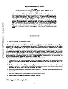
Table 1: Comparison of numerical results from Recola (upper numbers) and Pole (lower NLO to the total cross section of various partonic process numbers) for the NLO contribution δσEW classed (summed over q = u, d). In addition to the complete NLO correction we separately give the finite virtual and real corrections and the relative differences between Recola and Pole. A more detailed comparison can be obtained by comparing the weights at individual phase space points. For 106 Monte-Carlo generated phase-space points we have compared the pure virtual contribution 2 Re(M∗LO δMNLO ) to the squared matrix element (with divergences omitted) calculated by Recola and Pole for the partonic process ug → ugZ. In Fig. 3 we show the integrated fraction of the 106 phase-space points for which the agreement |R/P − 1| between Recola and Pole is worse than ∆. We find a typical agreement of 10−11 − 10−14 , with less than 1% of the phase-space points showing an agreement worse than 10−7 and less than 0.02% showing an agreement worse than 10−5 . The result of this test of the precision of the code is similar to the one performed by the OpenLoops collaboration [57] which also uses the tensor-integral library Collier. Note, however, that we compare two independent codes for the calculation of the tensor coefficients which are based on two entirely different algorithms. Furthermore the distribution of the phase-space points is in our case determined from the multi-channel Monte Carlo generator adapted to the peaking structure of the underlying process. Finally, we give some details on timing and the amount of memory required. The evaluation of the spin- and colour summed one-loop matrix elements takes about 30 ms per phase-space point for ug → ugZ (or any other partonic process considered in this paper) on a single Intel i7-2720QM core with gfortran 4.6.1. The size of the executable on disk is about 3 MB. The matrix elements are constructed during the run and the required memory depends strongly on the size of the dynamically generated internal arrays and thus on the considered process. For pp → Z + 2 jets memory is no issue. More complicated processes will be considered in the future.

3.2 3.2.1

Numerical results Input parameters and selection cuts

We use the following set of input parameters [100], Gµ OS MW MZOS MH

= = = =

1.1663787 × 10−5 GeV−2 , 80.385 GeV, 91.1876 GeV, 125 GeV,

ΓOS W = 2.085 GeV, ΓOS Z = 2.4952 GeV, mt = 173.2 GeV

(3.7)

with the value for the top-quark mass taken from Ref. [101]. The pole masses MW,Z and widths OS according to ΓW,Z entering our calculation are obtained from the stated on-shell values MW,Z 17

100

fraction of events

10−1 10−2 10−3 10−4 10−5 10−6 10−16

10−12

10−8

10−4

10−0

maximum accuracy ∆

Figure 3: Level of agreement of 2 Re(M∗LO δMNLO ) between Recola and Pole for ug → ugZ. The plot shows the probability for an agreement worse than ∆ for 106 phase-space points generated by the Monte Carlo. (3.4). The electromagnetic coupling constant αGµ is determined from Gµ via (3.5). The CKM matrix only appears in loop amplitudes and is set to unity. For the prediction of the hadronic pp → Z + 2 jets cross section the partonic cross sections have to be convoluted with the corresponding parton distribution functions (PDFs). Since our calculation does not take into account NLO QCD effects, we consistently resort to LO PDFs, using the LHAPDF implementation of the central MSTW2008LO PDF set [102]. From there we infer the value αLO (3.8) s (MZ ) = 0.1394 for the strong coupling constant. We identify the QCD factorisation scale µF and the renormalisation scale µR choosing µF = µR = MZ . (3.9) Note that the choice of the scales µF,R as well as the actual value for the strong coupling αs plays a minor role for our numerical analysis of EW radiative corrections in Section 3.2.2. We focus on NLO /σ LO from which the relative importance of the NLO EW corrections considering the ratio σEW the αs - and the scale dependence drop out. For the jet-reconstruction we use the anti-kT clustering algorithm [103] with separation parameter R = 0.4. For our scenario with exactly two partons and one potential photon in q the final state this simply amounts to recombining the photon with a parton a if Raγ = (ya − yγ )2 + φ2aγ < R. Here y = 21 ln[(E + pL )/(E − pL )] is the particle’s rapidity with E denoting its energy and pL its three-momentum component along the beam axis, and φaγ is the azimuthal angle between the the photon and the parton a in the plane transverse to the beam axis. In case of recombination, the resulting photon–parton jet is subjected to the cut zγ = Eγ /(Eγ + Ea ) < 0.7 in order to distinguish between Z + 2 jets and Z + 1 jet + γ production as explained in Section 3.1.3. After a possible recombination, we require two hard jets with pT,jet > 25 GeV, 18

|yjet | < 4.5

(3.10)

LO [%] σ LO /σtot

NLO [pb] σEW

1324.1(2)

68.79

1308.8(2)

−1.16

128.84(2)

6.69

127.56(2)

87.40(2)

4.54

86.18(2)

−0.99

88.41(2)

4.59

—

—

87.98(2)

4.57

—

—

16.566(3)

0.86

—

—

111.74(3)

5.81

—

—

79.70(2)

4.14

—

—

gluonic

1540.4(2)

80.02

1522.5(2)

four-quark

384.41(4)

19.98

—

−1.16

sum

1924.8(2)

100.00

—

ug → ugZ, dg → dgZ, ¯ → dgZ ¯ u ¯g → u ¯gZ, dg ¯ → ggZ u¯ u → ggZ, dd ¯ gg → u¯ uZ, gg → ddZ

uu′

NLO σEW σLO

σ LO [pb]

Process class

uu′ Z,

dd′

dd′ Z,

→ → ′ ′ ¯d ¯ →d ¯d ¯′Z →u ¯u ¯ Z, d ¯ → d′ d ¯′ Z, u¯ u → u′ u ¯′ Z, dd ¯ ′ → dd ¯′ Z u¯ u′ → u¯ u′ Z, dd u ¯u ¯′

¯ dd ¯ → u¯ u¯ u → ddZ, uZ, ′ ′ ′ ¯ ¯ u¯ u → dd Z, dd → u¯ u′ Z ¯→u ¯′ Z, ud → u′ d′ Z, u ¯d ¯′ d ¯→u ¯ ud → udZ, u ¯d ¯dZ ¯ → u′ d ¯′ Z, u ud ¯d → u ¯′ d′ Z, ¯ → udZ, ¯ u ud ¯d → u ¯dZ

− 1 [%]

−1.37

—

—

Table 2: Composition of the LO cross section for pp → Z + 2 jets at the 8 TeV LHC. In the first column the partonic processes are listed, where u, u′ denote the up-type quarks u, c and d, d′ the down-type quarks d, s, b. The second column provides the corresponding cross section where the numbers in parenthesis give the integration error on the last digit. The third column contains the relative contribution to the total cross section in percent. In the fourth column we list the NLO EW cross section for the gluonic channels and in the last column the relative EW corrections. for the final event. 3.2.2

Results

In this section we present results for the total cross section and various differential distributions using the numerical input parameters and acceptance cuts introduced above. The total cross section and its composition at LO for the 8 TeV LHC is shown in Table 2 where the absolute and relative contributions of the partonic channels are listed. In the lower part of Table 2 we provide the contribution to the total cross section of partonic processes with external gluons (gluonic) and of the four-quark processes (four-quark). We find the total cross section dominated by processes with external gluons, in particular by the quark-gluon induced processes (69%). We also provide the NLO cross section and the relative EW corrections for the gluonic channels in the last two columns of Table 2. For our set of cuts, they range between −1.0% and −1.4% for the different gluonic channels. In the following we present results for distributions at LO and NLO for the gluonic channels only. Although these channels dominate the total cross section we emphasise that there are

19

105

105 LO

NLO

NLO

104 103

103

102

102

101

101

100

0

10−1

10−1

10−2

10

1

1

0.8 1000

0.8 250

500

750

250

1000

500

750

pT,j2 [GeV]

pT,j1 [GeV] 4 · 105 3 · 105

LO

LO

NLO

NLO

4 · 105 3 · 105

2 · 105

2 · 105

1 · 105

1 · 105

0 · 100

0 · 100

1

dσ [fb] dy j2

dσ [fb] dy j1

dσ [fb/GeV] dpT,j2

dσ [fb/GeV] dpT,j1

104

LO

1

0.99

0.99

0.98

0.98 −4

−3

−2

−1

0

1

2

3

4

−4

yj1

−3

−2

−1

0

1

2

3

4

yj2

Figure 4: Distributions of the transverse momentum and the rapidity of the harder jet j1 and the softer jet j2 at the 8 TeV LHC at LO (blue, dashed) and NLO (red, solid). The lower panels show the ratio of the NLO distribution over the LO distribution. certain phase-space regions where the relative importance of the four-quark processes is enhanced and these channels and the corresponding EW corrections should not be neglected to describe pp → Z + 2 jets properly. For each distribution we provide two plots: the upper panels show the LO and NLO prediction for the differential cross section while the lower panels show the NLO result normalised to the LO result. In Fig. 4 we present results for the differential cross section as a function of the transverse momentum and the rapidity for the harder jet j1 and softer jet j2 , respectively. Both transverse momentum distributions show steep slopes over six orders of magnitude in the displayed pT range. The EW corrections lower the LO prediction, and their relative size grows in absolute value with increasing transverse momentum due to the well-known EW Sudakov logarithms [104–107]. For transverse momenta of the softer jet pT,j2 ≃ 1 TeV the impact of EW corrections amounts up to −10% relative to the Born approximation, while for transverse momenta of the harder jet pT,j1 ≃ 1 TeV the EW effects are of the order of −15%. Since, the rapidity distributions are not sensitive to Sudakov logarithms, the corresponding EW corrections are flat and around −1% as for the total cross section. The differential cross section as a function of the di-jet invariant mass and as a function of the transverse momentum of the Z boson is shown on the left-hand side in Fig. 5. For both distributions we find the expected dependence on the Sudakov logarithms, although the sensitivity in the di-jet invariant-mass distribution is less pronounced than in the pT,Z -distribution. For Mjj ≃ 500 GeV the EW corrections are of the order of −2%; they amount up to −4% for Mjj ≃2 TeV. The transverse momentum distribution of the Z boson receives large corrections, 20

LO

LO

103

NLO

NLO

1 · 106 1 · 106

102

8 · 105

101

6 · 105

100

4 · 105

10−1

2 · 105

dσ [fb] dφjj

dσ [fb/GeV] dMjj

104

1

1

0.99 0.9 0

500

1000

1500

π 4

2000 0

3π 4

π

φjj

Mjj [GeV] 104

LO

103

NLO

3 · 105

102

2 · 105

LO

101

NLO 1 · 105

100 10

dσ [fb] dyZ

dσ [fb/GeV] dpT,Z

0.98

π 2

−1

10−2

0 · 100

1

1 0.99

0.8

0.98 250

500

750

1000

pT,Z [GeV]

−4

−3

−2

−1

0

1

2

3

4

yZ

Figure 5: Distributions of the di-jet invariant mass, the relative azimuthal angle between the two jets, the transverse momentum and the rapidity of the Z boson at the 8 TeV LHC at LO (blue, dashed) and NLO (red, solid). The lower panels show the ratio of the NLO distribution over the LO distribution. from −15% for pT,Z ≃ 500 GeV to −25% for pT,Z ≃ 1 TeV. On the upper right-hand side in Fig. 5 we present the differential distribution of the relative azimuthal angle φjj between the two jets. The φjj -distribution shows that the two jets are preferably back-to-back in the transverse plane and that the EW corrections lower the differential cross section by 1−1.5%. They induce a shape change at the permille level relative to the LO approximation. The rapidity distribution of the Z boson is depicted in the lower right-hand side of Fig. 5. In the central region |yZ | < 2, where most of the Z bosons are produced, the EW corrections lower the LO cross section by 1−1.5% while for |yZ | > 2 their effect drops to the permille level.

4

Conclusions

The full exploitation of the Large Hadron Collider relies on precise theoretical predictions. To this end QCD and electroweak next-to-leading order corrections have to be calculated for many processes involving many particles in the final state. This requires efficient and reliable automatic tools. In this paper we have presented Recola, a Fortran90 code for the REcursive Computation of One-Loop Amplitudes. It uses methods based on Dyson–Schwinger equations to calculate the coefficients of all tensor integrals appearing in a one-loop amplitude recursively. The tensor integrals can then be evaluated with efficient numerically stable techniques. The algorithm has

21

been implemented for the full electroweak Standard Model, including counterterms and rational terms, but could be generalised to more complicated theories in a straightforward way. The implementation supports the complex-mass scheme and is thus applicable to processes involving intermediate unstable particles. For the treatment of colour we have developed a new recursive algorithm based on colour structures that naturally appear in the colour-flow representation. As a first application of Recola, we have calculated the electroweak corrections to the dominant partonic channels in Z + 2 jets production at the LHC. The results have been verified with an independent calculation based on Feynman-diagrammatic methods. For a typical set of cuts, the electroweak corrections are negative at the level of one percent, but become sizeable where large energy scales are relevant. However, in general and in particular for large energies of the jets, a meaningful prediction requires the inclusion of next-to-leading-order corrections to all partonic channels. This will be pursued in a forthcoming publication.

Acknowledgements We are grateful to S. Pozzorini for many useful discussions and to A. M¨ uck for help concerning Pole. This work was supported in part by the Swiss National Science Foundation (SNF) under contract 200021-126364, by the Deutsche Forschungsgemeinschaft (DFG) under reference number DE 623/2-1, and by the Helmholtz alliance “Physics at the Terascale”.

References [1] M. Ciccolini, A. Denner and S. Dittmaier, Phys. Rev. D 77 (2008) 013002 [arXiv:0710.4749 [hep-ph]]. [2] Z. Bern, L. J. Dixon, D. C. Dunbar and D. A. Kosower, Nucl. Phys. B 425 (1994) 217 [hep-ph/9403226]. [3] Z. Bern, L. J. Dixon, D. C. Dunbar and D. A. Kosower, Nucl. Phys. B 435 (1995) 59 [hep-ph/9409265]. [4] R. Britto, F. Cachazo and B. Feng, Nucl. Phys. B 725 (2005) 275 [hep-th/0412103]. [5] G. Ossola, C. G. Papadopoulos and R. Pittau, Nucl. Phys. B 763 (2007) 147 [hep-ph/0609007]. [6] G. Ossola, C. G. Papadopoulos and R. Pittau, JHEP 0707 (2007) 085 [arXiv:0704.1271 [hep-ph]]. [7] R. K. Ellis, W. T. Giele and Z. Kunszt, JHEP 0803 (2008) 003 [arXiv:0708.2398 [hep-ph]]. [8] W. T. Giele, Z. Kunszt and K. Melnikov, JHEP 0804 (2008) 049 [arXiv:0801.2237 [hep-ph]]. [9] R. K. Ellis, W. T. Giele, Z. Kunszt and K. Melnikov, Nucl. Phys. B 822 (2009) 270 [arXiv:0806.3467 [hep-ph]]. [10] G. Passarino and M. J. G. Veltman, Nucl. Phys. B 160 (1979) 151. [11] C. F. Berger, Z. Bern, L. J. Dixon, F. Febres Cordero, D. Forde, H. Ita, D. A. Kosower and D. Maˆıtre, Phys. Rev. D 78 (2008) 036003 [arXiv:0803.4180 [hep-ph]]. [12] W. T. Giele and G. Zanderighi, JHEP 0806 (2008) 038 [arXiv:0805.2152 [hep-ph]]. 22

[13] A. Lazopoulos, arXiv:0812.2998 [hep-ph]. [14] W. Giele, Z. Kunszt and J. Winter, Nucl. Phys. B 840 (2010) 214 [arXiv:0911.1962 [hep-ph]]. [15] S. Badger, B. Biedermann and P. Uwer, Comput. Phys. Commun. 182 (2011) 1674 [arXiv:1011.2900 [hep-ph]]. [16] V. Hirschi, R. Frederix, S. Frixione, M. V. Garzelli, F. Maltoni and R. Pittau, JHEP 1105 (2011) 044 [arXiv:1103.0621 [hep-ph]]. [17] G. Bevilacqua, M. Czakon, M. V. Garzelli, A. van Hameren, A. Kardos, C. G. Papadopoulos, R. Pittau and M. Worek, arXiv:1110.1499 [hep-ph]. [18] G. Cullen, N. Greiner, G. Heinrich, G. Luisoni, P. Mastrolia, G. Ossola, T. Reiter and F. Tramontano, Eur. Phys. J. C 72 (2012) 1889 [arXiv:1111.2034 [hep-ph]]. [19] C. F. Berger, Z. Bern, L. J. Dixon, F. Febres Cordero, D. Forde, T. Gleisberg, H. Ita and D. A. Kosower et al., Phys. Rev. D 80 (2009) 074036 [arXiv:0907.1984 [hep-ph]]. [20] R. K. Ellis, K. Melnikov and G. Zanderighi, Phys. Rev. D 80 (2009) 094002 [arXiv:0906.1445 [hep-ph]]. [21] C. F. Berger, Z. Bern, L. J. Dixon, F. Febres Cordero, D. Forde, T. Gleisberg, H. Ita and D. A. Kosower et al., Phys. Rev. Lett. 102 (2009) 222001 [arXiv:0902.2760 [hep-ph]]. [22] G. Bevilacqua, M. Czakon, C. G. Papadopoulos, R. Pittau and M. Worek, JHEP 0909 (2009) 109 [arXiv:0907.4723 [hep-ph]]. [23] K. Melnikov and G. Zanderighi, Phys. Rev. D 81 (2010) 074025 [arXiv:0910.3671 [hep-ph]]. [24] G. Bevilacqua, M. Czakon, C. G. Papadopoulos and M. Worek, Phys. Rev. Lett. 104 (2010) 162002 [arXiv:1002.4009 [hep-ph]]. [25] C. F. Berger, Z. Bern, L. J. Dixon, F. Febres Cordero, D. Forde, T. Gleisberg, H. Ita and D. A. Kosower et al., Phys. Rev. D 82 (2010) 074002 [arXiv:1004.1659 [hep-ph]]. [26] T. Melia, K. Melnikov, R. Rontsch and G. Zanderighi, JHEP 1012 (2010) 053 [arXiv:1007.5313 [hep-ph]]. [27] C. F. Berger, Z. Bern, L. J. Dixon, F. Febres Cordero, D. Forde, T. Gleisberg, H. Ita and D. A. Kosower et al., Phys. Rev. Lett. 106 (2011) 092001 [arXiv:1009.2338 [hep-ph]]. [28] G. Bevilacqua, M. Czakon, A. van Hameren, C. G. Papadopoulos and M. Worek, JHEP 1102 (2011) 083 [arXiv:1012.4230 [hep-ph]]. [29] T. Melia, K. Melnikov, R. Rontsch and G. Zanderighi, Phys. Rev. D 83 (2011) 114043 [arXiv:1104.2327 [hep-ph]]. [30] R. Frederix, S. Frixione, V. Hirschi, F. Maltoni, R. Pittau and P. Torrielli, JHEP 1109 (2011) 061 [arXiv:1106.6019 [hep-ph]]. [31] H. Ita, Z. Bern, L. J. Dixon, F. Febres Cordero, D. A. Kosower and D. Maˆıtre, Phys. Rev. D 85 (2012) 031501 [arXiv:1108.2229 [hep-ph]].

23

[32] G. Bevilacqua, M. Czakon, C. G. Papadopoulos and M. Worek, Phys. Rev. D 84 (2011) 114017 [arXiv:1108.2851 [hep-ph]]. [33] Z. Bern, G. Diana, L. J. Dixon, F. Febres Cordero, S. H¨oche, D. A. Kosower, H. Ita and D. Maˆıtre et al., Phys. Rev. Lett. 109 (2012) 042001 [arXiv:1112.3940 [hep-ph]]. [34] N. Greiner, G. Heinrich, P. Mastrolia, G. Ossola, T. Reiter and F. Tramontano, Phys. Lett. B 713 (2012) 277 [arXiv:1202.6004 [hep-ph]]. [35] G. Bevilacqua and M. Worek, JHEP 1207 (2012) 111 [arXiv:1206.3064 [hep-ph]]. [36] S. Badger, B. Biedermann, P. Uwer and V. Yundin, arXiv:1209.0098 [hep-ph]. [37] J. Alcaraz Maestre et al. [SM AND NLO MULTILEG and SM MC Working Groups Collaboration], arXiv:1203.6803 [hep-ph]. [38] D. E. Soper, Phys. Rev. D 62 (2000) 014009 [hep-ph/9910292]. [39] S. Becker, C. Reuschle and S. Weinzierl, JHEP 1012 (2010) 013 [arXiv:1010.4187 [hep-ph]]. [40] S. Becker, D. Goetz, C. Reuschle, C. Schwan and S. Weinzierl, Phys. Rev. Lett. 108 (2012) 032005 [arXiv:1111.1733 [hep-ph]]. [41] G. Ossola, C. G. Papadopoulos and R. Pittau, JHEP 0803 (2008) 042 [arXiv:0711.3596 [hep-ph]]. [42] P. Mastrolia, G. Ossola, T. Reiter and F. Tramontano, JHEP 1008 (2010) 080 [arXiv:1006.0710 [hep-ph]]. [43] G. Heinrich, G. Ossola, T. Reiter and F. Tramontano, JHEP 1010 (2010) 105 [arXiv:1008.2441 [hep-ph]]. [44] R. Pittau, Comput. Phys. Commun. 181 (2010) 1941 [arXiv:1006.3773 [hep-ph]]. [45] A. Ferroglia, M. Passera, G. Passarino and S. Uccirati, Nucl. Phys. B 650 (2003) 162 [hep-ph/0209219]. [46] A. Denner and S. Dittmaier, Nucl. Phys. B 658 (2003) 175 [hep-ph/0212259]. [47] T. Binoth, J. P. Guillet, G. Heinrich, E. Pilon and C. Schubert, JHEP 0510 (2005) 015 [hep-ph/0504267]. [48] A. Denner and S. Dittmaier, Nucl. Phys. B 734 (2006) 62 [hep-ph/0509141]. [49] A. Bredenstein, A. Denner, S. Dittmaier and M. M. Weber, JHEP 0702 (2007) 080 [hep-ph/0611234]. [50] A. Denner, S. Dittmaier, T. Kasprzik and A. M¨ uck, JHEP 0908 (2009) 075 [arXiv:0906.1656 [hep-ph]]. [51] A. Denner, S. Dittmaier, T. Kasprzik and A. M¨ uck, JHEP 1106 (2011) 069 [arXiv:1103.0914 [hep-ph]]. [52] A. Denner, S. Dittmaier, S. Kallweit and A. M¨ uck, JHEP 1203 (2012) 075 [arXiv:1112.5142 [hep-ph]]. 24

[53] A. Bredenstein, A. Denner, S. Dittmaier and S. Pozzorini, Phys. Rev. Lett. 103 (2009) 012002 [arXiv:0905.0110 [hep-ph]]. [54] A. Denner, S. Dittmaier, S. Kallweit and S. Pozzorini, Phys. Rev. Lett. 106 (2011) 052001 [arXiv:1012.3975 [hep-ph]]. [55] F. Campanario, C. Englert, M. Rauch and D. Zeppenfeld, Phys. Lett. B 704 (2011) 515 [arXiv:1106.4009 [hep-ph]]. [56] L. Reina and T. Schutzmeier, JHEP 1209 (2012) 119 [arXiv:1110.4438 [hep-ph]]. [57] F. Cascioli, P. Maierhofer and S. Pozzorini, Phys. Rev. Lett. 108 (2012) 111601 [arXiv:1111.5206 [hep-ph]]. [58] A. van Hameren, JHEP 0907 (2009) 088 [arXiv:0905.1005 [hep-ph]]. [59] F. A. Berends and W. T. Giele, Nucl. Phys. B 306 (1988) 759. [60] J. M. Campbell and R. K. Ellis, Phys. Rev. D 65 (2002) 113007 [hep-ph/0202176]. [61] J. M. Campbell, R. K. Ellis and D. L. Rainwater, Phys. Rev. D 68 (2003) 094021 [hep-ph/0308195]. [62] C. Oleari and D. Zeppenfeld, Phys. Rev. D 69 (2004) 093004 [hep-ph/0310156]. [63] F. J. Dyson, Phys. Rev. 75 (1949) 1736. [64] J. S. Schwinger, Proc. Nat. Acad. Sci. 37 (1951) 452. [65] J. S. Schwinger, Proc. Nat. Acad. Sci. 37 (1951) 455. [66] A. Kanaki and C. G. Papadopoulos, Comput. Phys. Commun. 132 (2000) 306 [hep-ph/0002082]. [67] C. G. Papadopoulos and M. Worek, Eur. Phys. J. C 50 (2007) 843 [hep-ph/0512150]. [68] A. Cafarella, C. G. Papadopoulos and M. Worek, Comput. Phys. Commun. 180 (2009) 1941 [arXiv:0710.2427 [hep-ph]]. [69] K. Hagiwara and D. Zeppenfeld, Nucl. Phys. B 313 (1989) 560. [70] F. Caravaglios and M. Moretti, Phys. Lett. B 358 (1995) 332 [hep-ph/9507237]. [71] G. Ossola, C. G. Papadopoulos and R. Pittau, JHEP 0805 (2008) 004 [arXiv:0802.1876 [hep-ph]]. [72] P. Draggiotis, M. V. Garzelli, C. G. Papadopoulos and R. Pittau, JHEP 0904 (2009) 072 [arXiv:0903.0356 [hep-ph]]. [73] M. V. Garzelli, I. Malamos and R. Pittau, JHEP 1001 (2010) 040 [Erratum-ibid. 1010 (2010) 097] [arXiv:0910.3130 [hep-ph]]. [74] H. -S. Shao, Y. -J. Zhang and K. -T. Chao, JHEP 1109 (2011) 048 [arXiv:1106.5030 [hepph]]. [75] A. Denner, Fortsch. Phys. 41 (1993) 307 [arXiv:0709.1075 [hep-ph]]. 25

[76] A. Denner, S. Dittmaier, M. Roth and D. Wackeroth, Nucl. Phys. B 560 (1999) 33 [hep-ph/9904472]. [77] A. Denner, S. Dittmaier, M. Roth and L. H. Wieders, Nucl. Phys. B 724 (2005) 247 [Erratum-ibid. B 854 (2012) 504] [hep-ph/0505042]. [78] Z. Bern and D. A. Kosower, Nucl. Phys. B 362 (1991) 389. [79] G. ’t Hooft, Nucl. Phys. B 72 (1974) 461. [80] A. Kanaki and C. G. Papadopoulos, hep-ph/0012004. [81] F. Maltoni, K. Paul, T. Stelzer and S. Willenbrock, Phys. Rev. D 67 (2003) 014026 [hep-ph/0209271]. [82] A. Denner and S. Dittmaier, Nucl. Phys. Proc. Suppl. 160 (2006) 22 [hep-ph/0605312]. [83] D. Y. Bardin, A. Leike, T. Riemann and M. Sachwitz, Phys. Lett. B 206 (1988) 539. [84] W. Beenakker and A. Denner, Nucl. Phys. B 338 (1990) 349. [85] A. Denner, U. Nierste and R. Scharf, Nucl. Phys. B 367 (1991) 637. [86] A. Denner and S. Dittmaier, Nucl. Phys. B 844 (2011) 199 [arXiv:1005.2076 [hep-ph]]. [87] S. Dittmaier and M. Kr¨ amer, Phys. Rev. D 65 (2002) 073007 [hep-ph/0109062]. [88] S. Catani and M. H. Seymour, Nucl. Phys. B 485 (1997) 291 [Erratum-ibid. B 510 (1998) 503] [hep-ph/9605323]. [89] A. Denner, S. Dittmaier, T. Gehrmann and C. Kurz, Nucl. Phys. B836 (2010) 37 [arXiv:1003.0986 [hep-ph]]. [90] E. W. N. Glover and A. G. Morgan, Z. Phys. C 62 (1994) 311. [91] D. Buskulic et al. [ALEPH Collaboration], Z. Phys. C 69 (1996) 365. [92] A. Denner, S. Dittmaier and L. Hofer, in preparation. [93] T. Motz, PhD thesis, Z¨ urich 2011. [94] T. Hahn, Comput. Phys. Commun. 140 (2001) 418 [hep-ph/0012260]. [95] T. Hahn and C. Schappacher, Comput. Phys. Commun. 143 (2002) 54 [hep-ph/0105349]. [96] T. Hahn and M. P´erez-Victoria, Comput. Phys. Commun. 118 (1999) 153 [hep-ph/9807565]. [97] S. Dittmaier, Phys. Rev. D 59 (1999) 016007 [hep-ph/9805445]. [98] E. Accomando, A. Denner and C. Meier, Eur. Phys. J. C 47 (2006) 125 [hep-ph/0509234]. [99] S. Dittmaier and M. Roth, Nucl. Phys. B 642 (2002) 307 [hep-ph/0206070]. [100] J. Beringer et al. [Particle Data Group Collaboration], Phys. Rev. D 86 (2012) 010001. [101] [Tevatron Electroweak Working Group and CDF and D0 Collaborations], arXiv:1107.5255 [hep-ex]. 26

[102] A. D. Martin et al., Eur. Phys. J. C 63, (2009) 189 [arXiv:0901.0002 [hep-ph]]. [103] M. Cacciari, G. P. Salam and G. Soyez, JHEP 0804 (2008) 063 [arXiv:0802.1189 [hep-ph]]. [104] P. Ciafaloni and D. Comelli, Phys. Lett. B 446 (1999) 278 [hep-ph/9809321]. [105] J. H. K¨ uhn and A. A. Penin, hep-ph/9906545. [106] V. S. Fadin, L. N. Lipatov, A. D. Martin and M. Melles, Phys. Rev. D 61 (2000) 094002 [hep-ph/9910338]. [107] A. Denner and S. Pozzorini, Eur. Phys. J. C 18 (2001) 461 [hep-ph/0010201].

27