Recursive Frechet Mean Computation on the Grassmannian and its ...

Recursive Fr´echet Mean Computation on the Grassmannian and its Applications to Computer Vision Rudrasis Chakraborty and Baba C. Vemuri Department of CISE, University of Florida Gainesville, FL 32611, USA {rudrasis, vemuri}@cise.ufl.edu Abstract

In the past decade, Grassmann manifolds (Grassmannian) have been commonly used in mathematical formulations of many Computer Vision tasks. Averaging points on a Grassmann manifold is a very common operation in many applications including but not limited to, tracking, action recognition, video-face recognition, face recognition, etc. Computing the intrinsic/Fr´echet mean (FM) of a set of points on the Grassmann can be cast as finding the global optimum (if it exists) of the sum of squared geodesic distances cost function. A common approach to solve this problem involves the use of the gradient descent method. An alternative way to compute the FM is to develop a recursive/inductive definition that does not involve optimizing the aforementioned cost function. In this paper, we propose one such computationally efficient algorithm called the Grassmann inductive Fr´echet mean estimator (GiFME). In developing the recursive solution to find the FM of the given set of points, GiFME exploits the fact that there is a closed form solution to find the FM of two points on the Grassmann. In the limit as the number of samples tends to infinity, we prove that GiFME converges to the FM (this is called the weak consistency result on the Grassmann manifold). Further, for the finite sample case, in the limit as the number of sample paths (trials) goes to infinity, we show that GiFME converges to the finite sample FM. Moreover, we present a bound on the geodesic distance between the estimate from GiFME and the true FM. We present several experiments on synthetic and real data sets to demonstrate the performance of GiFME in comparison to the gradient descent based (batch mode) technique. Our goal in these applications is to demonstrate the computational advantage and achieve comparable accuracy to the state-of-the-art.

1. Introduction The Grassmann manifold has been commonly used in mathematical formulations of many computer vision tasks such as video based face recognition [34, 4], activity recognition [5, 35], video restoration [15], shape analysis [13, 25] etc. Given a set of data points on a Grassmann manifold, finding their average is a crucial task in many classification and clustering based applications including the aforementioned applications. Since, a general Riemannian manifold lacks vector space structure, a Euclidean mean is not a valid representative of the average of points on the manifold. Instead one can use a Riemannian center of mass, also known as the Fr´echet mean (FM) [12, 18] as a way to denote the average of data points. This mean however is not unique in general and can be shown to be unique only in a geodesic ball of a certain injectivity/convexity radius. We refer the reader to an excellent paper [2] for a detailed exposition on this topic. Further, in general there is no closed form solution for the FM of an arbitrary number of points on a Riemannian manifold. Of course, one can argue about using the Euclidean mean which though computationally efficient, is not intrinsic and does not have many of the desired properties of the FM on the manifold. On a Riemannian manifold, the FM is defined as the minimizer of the sum of squared geodesic distances cost function. A popular approach to compute the FM is to use a gradient descent technique on this cost function [10, 24, 3]. An alternative approach to finding the FM proposed in [14] however does not involve the minimization of a cost function but is posed as a special case of iteratively finding the zeros of a vector field on the Riemannian manifold. Where applicable, a recursive algorithm can take advantage of the closed form solution to compute the FM of two points as the base of the recursion and recurse through the number of points in the given set. This will yield a much faster way to compute the FM if and when the convergence of the algorithm can be proved. In [31], an inductive definition of FM was proposed and almost sure convergence

4229

was shown for all non-positively curved (NPC) spaces. In [33], authors also presented a recursive FM computation algorithm but without any convergence analysis. Recently, recursive algorithms (along with proofs of convergence) to compute the FM on the Riemannian manifold of (n × n) symmetric positive definite matrices (Pn ) were reported in [16, 27, 21]. In this paper, we present a novel recursive (also called inductive) algorithm with convergence analysis, for computing the FM on a Grassmann manifold whose geometry is quite distinct from that of Pn and hence the convergence analysis on Pn [16, 27, 21] does not carry over to this setting. The Grassmann manifold, denoted by Grass(p, n), is the space of p dimensional subspaces of Rn . In some of the recent works [34], researchers have used Procrustes metric defined in the ambient Euclidean space [7] instead of using an canonical metric on the Grassmann. As Grass(p, n) is geodesically complete, hence, by the Hopf-Rinow theorem [17], there exists at least one length minimizing geodesic between any two points on Grass(p, n). In our formulation, we use this closed form expression for geodesics derived using the unique (up to a multiplicative constant) unitary invariant Riemannian metric on the Grassmann [9, 1]. Note that in Euclidean space, the recursive form of computing the arithmetic mean (which yields the same solution as the minimization of sum of squared distances) involves only two points in each recursion step and can be geometrically interpreted as moving an appropriate distance away from the already computed mean (old mean) towards the new-mean on the straight line joining the old mean and the new data point. This geometric procedure can be readily extended to any Riemannian manifold using geodesics. To this end, we make use of the closed form expression – derived using the cannonical metric on the Grassman – for the geodesic between two points on the Grassman. More precisely, after computing the estimate of the FM of k points, denoted by Mk , the k + 1th estimate lies on the geodesic between Mk and the k + 1th point Xk+1 . This readily yields an algorithm for computing the FM that does not require any function optimization, a considerable advantage often realized as gains in computation time of several orders in magnitude over non-incremental algorithms based on minimization of sum of squared geodesic distances. However, because of the presence of curvature, the recursive form and the minimization formulation do not necessarily yield the same solution in general. In particular, it is not immediately clear that Mk will indeed converge asymptotically to the true FM. In this paper, we present a weak consistency result which implies that as the number of samples goes to infinity, our inductive estimator does converge to the Fr´echet expectation. For the finite samples case, with a fixed number of sample paths (trials), our estimator and FM in general can

be different but close. Hence, we also give the bound on the distance between our estimator and the finite sample FM. An excellent research monograph on the topic of statistics on special matrix manifolds including the Grassmann and Stiefel manifolds is the book by Chikuse [7]. The book however does not address computational efficiency issues. One of the first detailed and complete works on the gradient descent and the conjugate gradient descent algorithm on the Grassmann manifold was reported in [9]. Srivastava et al. [30] pose the commonly encountered Computer Vision problem of the subspace tracking problem on a complex Grassmann manifold. A nonlinear mean shift algorithm on the Grassmann manifold was presented in [32, 6] with applications to segmentation of multiple motions and filtering. Turaga et al. [34] have reported results on statistical analysis on the Grassmann manifold with various applications including action recognition, video face recognition etc. Most recently, Hauberg et al. [15] formulated the dimensionality reduction problem as an averaging problem on Grassmann. For a comprehensive survey of computer vision applications that use a variety of Riemannian manifolds including Grassmann we refer the reader to [23]. The rest of the paper is organized as follows. In section 2, we discuss the formulation of inductive FM on the Grassmann manifold. Further, we present a proof of the Weak Consistency of our estimator on the Grassmann. The distance between our inductive estimate of the FM and the true FM is also presented for the finite sample case. Experimental results on synthetic and real data sets are presented in section 3. Finally, in section 4, we draw conclusions.

2. Inductive Fr´echet mean on the Grassmann manifold In this section, we first briefly recall some preliminaries regarding the Grassmann manifold. Then, we present an inductive formulation for computing the Fr´echet mean (FM) [12, 18] on Grassmann manifold. For a finite sample set, the FM is defined as a minimizer of the sum of squared geodesic distances between the unknown mean and the given samples. In general, the uniqueness can only be guaranteed within a certain injectivity/ convexity radius [12, 18, 2]. We also prove the Weak Consistency of GiFME on the Grassmannian and present a bound on the distance between the the estimate obtained using GiFME and the FM.

2.1. Mathematical Preliminaries The set of all p−dimensional linear subspaces of Rn is defined as the Grassmann manifold, Grass(p, n), where p ∈ Z+ , n ∈ Z+ , n ≥ p. So, a point on Grass(p, n) is a p−dimensional hyperplane in Rn containing the origin. The special case of Grass(p, n) is when p = 1, which is called the real projective space. A point, X ∈ Grass(p, n)

4230

can be specified by a basis, i.e., a set of p, n−dimensional linearly independent vectors. Let Xn×p be the matrix whose columns are the basis vectors. Then, X = Col(X), where Col(X) returns the column space of X. The set of all n × p, p ≤ n, full rank matrices is termed as (noncompact) Stiefel manifold, denoted by St(p, n). Clearly, given X ∈ Grass(p, n), the choice of X ∈ St(p, n) for which X = Col(X) is not unique. In fact, Grass(p, n) can be identified with the quotient space St(p, n)/GL(p), where GL(p) is the p−dimensional general linear group, i.e., p × p non-singular matrices. Thus, GL(p) defines an equivalence relation on St(p, n) as follows: X ∼ Y iff ∃L ∈ GL(p) such that, X = Y L, X, Y ∈ St(p, n). Note that, Col(X) is same as Col(Y ), so the equivalence classes of St(p, n) are in one-to-one correspondence with the points on Grass(p, n). Now, we will consider the unitary group invariant canonical metric on Grass(p, n). The terminology used here is borrowed from [1]. In order to define a metric on Grass(p, n), we will first define a metric on St(p, n). Let X ∈ Grass(p, n), ξ, η ∈ TX Grass(p, n). Let, X ∈ St(p, n) such that X = Col(X). As St(p, n) is an open subset of Rn×p , TX St(p, n) is isomorphic to Rn×p . We define the horizontal space HX (a subspace of TX St(p, n)) as HX = {X ⊥ W |W ∈ R(n−p)×p } where X ⊥∈ St(n − p, n) s.t. X T X ⊥= 0. For any two U, V ∈ TX St(p, n) define the following metric:   hU, V iX = trace (X T X)−1 U T V (1)

According to the theory of principal fiber bundles [19], for every ξ ∈ TX Grass(p, n), there exists an unique horizontal vector ξ⋄X such that ξ⋄X projects to ξ via the span operation. Hence, using Eq. 1, we can define the metric on Grass(p, n) as follows:   T hξ, ηiX = trace (X T X)−1 ξ⋄X η⋄X (2)

where, ξ⋄X denotes the horizontal lift of ξ at X [1]. This metric is invariant under the orthogonal group (set of n × n dimensional orthogonal matrices) operation, i.e.,   T trace (X T X)−1 ξ⋄X η⋄X   = trace ((QX)T (QX))−1 (Qξ⋄X )T (Qη⋄X )

for all Q ∈ O(n). Further, it is well known that the Grassmann manifold is complete [1] and hence, one can extend the geodesics on it indefinitely. Given X , Y ∈ Grass(p, n) with their respective orthonormal basis (o.n.b.) X and Y , the unique geodesic, Γ(X , Y, t) from X to Y is defined by [1]:   Γ(X , Y, t) = span XV cos(Θt) + U sin(Θt) (3)

 I − XT Y is non-singular and  X(X T X)−1 X T Y (X T Y )−1 = U ΣV T be the “thin” Singular value decomposition (SVD), (i.e., U is n × p and V is p × p orthonormal matrix, whereas Σ is p × p diagonal matrix), and Θ = atanΣ. The geodesic distance between X and Y induced by the unitary invariant metric (as given in Eq. 2), is p (4) dGr (X , Y) = hξ, ξi

where,

−1 where, ξ = Exp−1 X Y, ExpX Y is the inverse of the Riemannian Exponential map. The distance between X and Y can also be shown as the 2−norm of diag(Θ), where, diag(Θ) returns the vector consisting of the diagonal elements of Θ (termed as principal angles between X and Y). Another classical definition of distance on Grassmannian is given by sin(max Θ), where max Θ is the largest principal angle. In this work, we have used the sin(max Θ) definition. We are now ready to use the above material to derive the incremental a.k.a inductive FM.

2.2. The Inductive Fr´echet Expectation Given the closed-form expression for the geodesic on a Grassmann manifold, now we are in a position to define the inductive Fr´echet expectation estimator on the Grassmann manifold, henceforth abbreviated as GiF EE. Prior to that, let us recall the definition of the Fr´echet Mean (FM) and the Fr´echet Expectation. The FM, X ∗ of a set of N points {X1 , · · · , XN }, is defined [12, 18] as: ∗

X = arg

min

Y∈Grass(p,n)

N X i=1

  d2Gr Y, Xi

(5)

For a probability density fX on Grass(p, n) with finite Riemannian L2 moment, the Fr´echet Expectation, µ∗ is defined [12, 18] as: Z   ∗ µ = arg min d2Gr µ, X fX (X )d(X ) µ∈Grass(p,n) Grass(p,n)

(6) where, d(X ) is the Riemannian measure (or volume form) used in defining the density on Grass(p, n). Algorithm for Inductive Fr´echet Expectation Estimator Let X1 , X2 , · · · be independent samples drawn from a probability distribution P (X ) on Grass(p, n). Then, we define the Fr´echet expectation estimator Mk by the following recursion:

Mk+1

M1 = X 1   = Γ Mk , Xk+1 , ωk+1

(7) (8)

where, Γ(., ., .) is the geodesic as defined in Eq. 3, and

4231

1 . Eq. 7 simply means that the k + 1th ωk+1 = k+1 estimator lies on the geodesic between the k th estimator and the k + 1th sample point. The rationale behind this formulation comes from the euclidean update formula as discussed in [16]. This inductive formulation will henceforth be denoted by GiF EE for expectation estimator and GiF M E for the finite sample mean estimator respectively. This simple inductive estimator can be shown to converge to the Fr´echet expectation as stated in Theorem 1. The proof of this theorem is given in the next subsection.

Theorem 1. (Weak Consistency): For any distribution P (X ) on Grass(p, n) with finite Riemannian L2 -moment, whose support is bounded by a geodesic ball of radius < π/4, and a sequence of independent samples X1 , X2 , · · · drawn from this distribution, the inductive Fr´echet expectation estimator (GiF EE) converges to the Fr´echet expectation in probability as the number of samples tends to ∞.

2.3. Proof of Theorem 1 In order to prove Theorem 1, i.e., the Weak Consistency of GiFEE on Grass(p, n), first we will prove three lemmas, which will be used to prove the Theorem 1. Note that these proof steps are not a part of our inductive algorithm. These steps are only needed to prove the weak consistency on Grass(p, n). Also, note that in the rest of paper with a slight abuse of notation, we have used the term ”geodesic” to denote the ”shortest geodesic”. Lemma 1. Let X and Y belong to Grass(p, n), n/2 > p, p > 1 and let X and Y be an orthonormal basis (o.n.b.) of X and Y respectively. Let the geodesic between X and Y be denoted by Γ(X , Y, t). Let A ∈ Mn×(n−1) (R) be of full column rank such that AT A = In−1 and AT X is of rank p. Then, ∃Xe, Ye ∈ Grass(p, n − 1) with their respective e and Ye such that Γ(X , Y, t) = span(AΓβ (t)) o.n.b. X e t). where Γβ (t) is a basis of Γ(Xe, Y,

Proof. : Since the distribution P (X ) has a support bounded by a geodesic ball of radius < π/4, the largest principal angle between X and Y is < π/2, i.e., X does not contain an orthogonal direction to Y, which implies X T Y is invertible.

i

th

T

where, xi is the i column of X. As Y Pand AA is not zero matrix, so Eq. 9 holds if either i ci xi = 0

i c i xi c i i xi =

Now, construct A ∈ Mn×(n−1) (R) as follows. Make the first p columns of A same as those of X. Then, we take each column of Y individually, and use Gram-Schmidt orthogonalization on that column. A is then augmented with this orthogonalized column. Note that, if a column of Y is in the columnspace of X, then, it is not used in the augmentation of A. After these operations, we fill the remaning columns of A by taking o.n.b. of Rn s.t. they together make A column orthonormal. Clearly, as the first p columns of A are all the columns of X, AT X is of full column rank. Hence, by the above claim, AT Y is of full column rank. Let, N ∈ Mp×p (R) be invertible matrix such that e X = AX

Y = AYe N

(10) (11)

e Ye ∈ M(n−1)×p (R) are column orthonormal. where, X, e Ye are o.n.b. of Hence, ∃ Xe, Ye ∈ Grass(p, n − 1) s.t. X, e e X , Y respectively. It’s easy   to see from our construction of I p e= A that X . Moreover, as Y ∈ Col(A), Ye N 0(n−1)×p gives the coefficient of the linear combination. Hence, we can use thin QR decomposition to get column orthonormal Ye and the upper-triangular N with a non-zero diagonal. e T Ye is invertible. Claim: X

e T Ye = Proof. : Using Equations 10 and 11, we get, X X T AAT Y N −1 . By our earlier claim, the square matrix, X T AAT Y is invertible. As product of invertible matrices e T Ye is invertible. is invertible, hence X 

Let Y (X T Y )−1 − X = U ΣV T be the SVD decomposition. Using the previous equalities and Equations 10 and 11, we get

Claim: Given the hypothesis as above, AT Y is of full column rank. Proof. : Consider the matrix R = X T AAT Y . Assume R is not of full rank, then ∃ {ci }pi=1 , not all 0 s.t., X ci xti (AAT )Y = 0 (9)

P

∈ N (AAT ). As X is of full column rank, 0 is true only if ci = 0, ∀i, which is a contradiction to our assumption that R is not P of full rank. Hence, P T T c x ∈ N (AA ), =⇒ AA i i i (ci xi ) = 0, =⇒ i AT X is not of full column rank, which is a contradiction to our hypothesis. Hence, R = X T AAT Y is invertible, =⇒ AT Y is of full column rank since, by hypothesis AT X is of full column rank.  or P

Y (X T Y )−1 − X

= = = =

e T AT AYe N )−1 − AX e AYe N (X
T −1 e Ye N ) − X e (12) A Ye N (X
−1 T −1 e Ye ) − X e (13) A Ye N N (X
e T Ye )−1 − X e A Ye (X (14)

e T Ye )−1 − X e = U eΣ e Ve T . Then, using EquaLet Ye (X tion 14, we obtain the relationship between (U, Σ, V ) and e , Σ, e Ve ) as follows: U = AU e , V = Ve and Σ = Σ. e Let (U 4232

e = atanΣ e = Θ. The geodesic between X Θ = atanΣ and Θ and Y , Γ(X , Y, t) can be expressed as [1]
¯ cos Θt + U sin Θt Γ(X , Y, t) = span XV (15)

Substituting the relationship between (U, Σ, V ) and e e Ve ) into Equation 15, we get (U , Σ,
¯ cos Θt + U sin Θt Γ(X , Y, t) = span XV  
e Ve cos Θt e +U e sin Θt e = span A X =

span(AΓβ (t))

(16)

e t). Thus, the geodesic where, Γβ (t) is the basis for Γ(Xe, Y, between X and Y in Grass(p, n) can be expressed as a function of Γβ (t). Note that AΓβ (t) is a basis for Γ(X , Y, t), and AT AΓβ (t) = Γβ (t) is of full column rank.  For, Grass(p, n) with p = n/2, if X and Y together spans Rn , ∄ A in Lemma 1. In this special case, instead of the reduction from Grass(p, n) to Grass(p, n − 1), we map from Grass(p, n) to Grass(p + 1, n). In this case, we look for a Xe, Ye ∈ Grass(p + 1, n) s.t., dGr (X , Y) = e So, in this case, we will get X = XB e and Y = dGr (Xe, Y). e Y C, where B and C contain the coefficient of the linear e and Ye respectively. Then, combination of columns of X we can use analogous arguments as in Lemma 1 to get the geodesic expression between X and Y from the geodesic e The detailed proof will be expression between Xe and Y. given in a future publication. .Lemma 2. Let X and Y belong to Grass(1, n) from a distribution whose support is bounded by geodesic ball of radius < π/4, and let X, Y ∈ S n−1 be the unit length basis of X and Y respectively s.t. dS (X, Y ) < π/2, where dS (., .) is the geodesic distance on S n−1 . Let ΓS (., ., t) denote the geodesic on S n−1 . Then, any point on the geodesic, at (t = t0 ), between X and Y , i.e., ΓS (X, Y, t0 ) spans Γ(X , Y, t0 ). Proof. Since X and Y are unit length basis, they lie on the hypersphere, S n−1 . Let Y (X T Y )−1 − X = U ΣV T be the SVD decomposition. Then, U ΣV T = Y (X T Y )−1 − X = Y −X cos θ , where, X T Y = cos θ and as X T Y is invertible cos θ thus, cos θ 6= 0. Then,

=

Y − X cos θ kY − X cos θk kY − X cos θk cos θ tan θ

(18)

=

1

(19)

U

=

Σ

=

V

(17)

So, atanΣ = θ. Using Equations 17-19, the geodesic Γ(X , Y, t) between X and Y, can be expressed as,
Γ(X , Y, t) = span XV cos θt + U sin θt
Y − X cos θ sin θt = span X cos θt + kY − X cos θk 
1  = span Y sin θt + X sin θ(1 − t) . sin θ (20) Since X, Y ∈ S n−1 , hence, Equation 20 implies that Γ(X , Y, t) = span(ΓS (X, Y, t)). Here, as ΓS (X, Y, t) ∈ S n−1 , hence, this becomes an unit length basis for the subspace on the geodesic between X and Y.  Lemma 3. Given the hypothesis as above, independent samples on Grass(p, n) induces independent samples ′ (from the induced distribution) on S n −1 for some n′ ≤ n. Proof. Consider a set of independent samples on Grass(p, n), X1 , · · · , XN . Using the proof of Lemma 1 and the claim within, we can take a full column orthonormal matrix A, to get samples X˜1 , · · · , X˜N on Grass(p, n − 1). Note that since any functional tranformation of indepedent samples yields independent samples (from the induced distribution), X˜1 , · · · , X˜N are independent samples. For the case when we need to go from Grass(p, n) to Grass(p + 1, n), by analogous argument, the samples are also independent. So, we will use the isometry between Grass(p, n) and Grass(n − p, n) [7], the reduction step from Grass(p, n) from Grass(p, n − 1) and the step from Grass(p, n) from Grass(p + 1, n) to get independent samples on Grass(1, n′ ), for some n′ ≤ n. ′ Now, define a mapping F : Grass(1, n′ ) → S n −1 by F(X ) = X ∗ sgn(Xn )/kXk, where X is a basis of X ∈ Grass(1, n′ ). Then, F induces independent samples on ′ S n −1 by the similar argument as before.  Given the above lemmas, we are now in a position to prove Theorem 1. Proof of Theorem 1. Given, Lemma 3, we can state that independent samples on Grass(p, n) induces independent ′ samples on S n −1 . Using Lemma 2, we can state that the geodesic on Grass(1, n) (between two points) can be computed from geodesic on S n−1 (between two corresponding points). And as our inductive FM computation algorithm, GiF EE, (in eqns. 7) requires closed form expression of the geodesic at each step, we can compute GiF EE of the samples on Grass(1, n) from the SiF EE on S n−1 . Moreover, using Lemma 1, we can also compute GiF EE on Grass(p, n) from the GiF EE on Grass(p, n − 1) as geodesic on Grass(p, n) can be computed from the geodesic on Grass(p, n − 1). For p = n/2 case, we will

4233

use the step to go from Grass(p, n) to Grass(p + 1, n). Additionally, we use the isometry between Grass(p, n) and Grass(n − p, n), n − p > 0 [7], to derive GiF EE on Grass(n − p, n) from the GiF EE on Grass(p, n). Hence, we can state that the GiF EE of the samples on ′ Grass(p, n) can be derived from the SiF EE on S n −1 , for some n′ ≤ n. Hence, given the proof of weak consistency ′ on S n −1 , we have a proof for the weak consistency of GiFEE on Grass(p, n). An example of the reduction steps from Grass(5, 10) to Grass(1, 4): Grass(5, 10) → Grass(6, 10) → Grass(4, 10) → Grass(4, 9) → Grass(4, 8) → Grass(5, 8) → Grass(3, 8) → Grass(3, 7) → Grass(3, 6) → Grass(4, 6) → Grass(2, 6) → Grass(2, 5) → Grass(2, 4) → Grass(3, 4) → Grass(1, 4), where → denotes the reduction step. We now state the weak consistency of our estimator on S n−1 in Theorem 2 and refer the reader to [26] for the proof.  Theorem 2. (Weak consistency on S n−1 ) Let Xi ’s be the independent samples drawn from a distribution whose support is bounded by a geodesic ball of radius < π/4. Then the inductive Fr´echet expectation estimator (SiF EE) will converge to the Fr´echet estimator in probability as the number of samples tend to ∞. In the next subsection, we will show convergence for finite sample set.

2.4. The Finite Sample Case Instead of infinite sample set, if we have finite sample set on Grass(p, n), it can also be proved that, if we draw an infinite number of times from the finite sample set, GiF M E converges to the FM of the finite samples. This result is analogous to Sturm’s result for non-positively curved (NPC) spaces [31] and proved for weighted inductive means on the manifold of symmetric positive definite matrices in Lim et. al [21]. Let X = {X1 , · · · , Xn } be the set of n points on Grass(p, n). Also, assume on X, FM exists and it is ∞ Y unique. Let, Nn = {1, · · · , n}. For each ω ∈ Nn , k=1

define inductively a sequence σω as follows: σω (1) = Xω(1)

1 σω (m) = Γ σω (m − 1), Xω(m) , m

!

This sequence may be viewed as a random walk starting at Xω(1) , and moving from σω (m − 1) toward Xω(m) along the geodesic to reach σω (m). Then, the following theorem holds.

Theorem 3. (Convergence of the inductive random walk) Given the hypothesis as above, as m → ∞, σω (m) converges almost surely to X ∗ , i.e., the FM of X. More concisely, lim σω (m) = X ∗ (21) m→∞

Proof. Let us construct a setYm = {Xω(1) , · · · , Xω(m) }. From Theorem 1, we can state that in the limit as m goes to ∞, σω (m) converges to the FM of Ym , which is same as the FM of the set X.  The more generalized form of Theorem 3, where associated with X there is a probability vector W = (w1 , w2 , · · · , wn ), is know as “no-dice theorem”, which is harder to prove. In our case, wi = n1 , ∀i. In the following subsection, we will present a bound on the distance between GiF M E and the finite sample FM.   2.5. An upper bound on dGr Mk+1 , X ∗

Given a finite number of sample points on Grass(p, n), let the k th estimate from GiF M E be Mk and the FM be denoted by X ∗ . Using Lemma 1 and the isometry between Grass(p, n) and Grass(n−p,  n), it is easy  to see that find-

ing an upper bound on dGr Mk+1 , X ∗ is equivalent to finding an upper bound on the distance between SiF M E and FM on S n−1 .

Lemma 4. Given S1 , · · · , Sn on northern hemisphere of S n−1 (i.e., nth coordinate of Si is always positive, ∀i) with FM S ∗ = (0, 0, · · · , 0, 1)t and k th inductive estimator, Tk , the distance between Tk and S ∗ , denoted by dS (Tk , S ∗ ) is bounded according to, dS (Tk , S ∗ ) ≤ max θ1i i

i where, θ1i , θ2i , · · · , θn−1 are the angular coordinates for Si , θji ∈ (0, π), ∀{i, j}.

The proof of this Lemma is given in [26].

3. Experimental Results In this section, we present experiments demonstrating the performance of GiFME in comparison to the batch mode counterpart (which uses the gradient descent on the sum of squared geodesic distances cost function) on synthetic and real data. Since the practical thrust of the paper is on computational efficiency in estimating the FM using GiFME, we provide the run times on a desktop used for performing all the experiments. All the experimental results reported here were executed on a desktop with a single 3.33 GHz Intel-i7 CPU with 24 GB RAM.

4234

0.45

4

GiFME GFME

0.4

GiFME GFME

3.5

0.35 3

Time taken (s)

Error

0.3

0.25

0.2

0.15

2.5

2

1.5

1 0.1

0.5

0.05

0

0 0

100

200

300

400

500

600

700

800

900

1000

0

100

200

300

400

Number of Samples

Figure 1. Average error comparison for GF M E and GiF M E

500

600

700

800

900

1000

Number of Samples

Figure 2. The running time comparison for GF M E and GiF M E (in an incremental context).

3.1. Comparative performance of GiFME on Synthetic data

900

GiFME GFME

800

700

# of samples required

We generate 1000 i.i.d. samples from a Log-Normal distribution on Grass(p, n) with variance 0.25 and expecta˜ where tion to be Col(I), ( 1 1≤i=j≤p I˜ij = 0 o.w.

600

500

400

300

200

100

0 0.1

0.09

0.08

0.07

0.06

0.05

0.04

0.03

0.02

0.01

dis(FM,*)

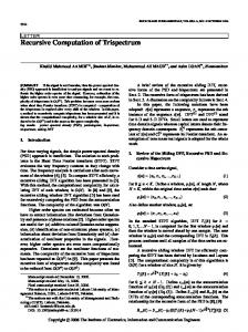
We use the procedure in [29] to generate samples form a Log-Normal distribution. Then, we input these i.i.d. samples to both GiF M E and GF M E (non-recursive, Grassman Fr´echet mean estimator). To compare the performance we compute the error, which is the intrinsic distance (on the Grassmann) between the computed mean and the FM. We also report the computation time for these both cases. We perform this experiment 10 times and the average error in accuracy and the average computation time are reported. The comparison plot of the average error is shown in Fig. 1, here n = 100, p = 10. In order to achieve faster convergence of GF M E, we have used the FM of k samples to initialize the FM computation for k + 1 samples. From this plot, it can be seen that the average accuracy error of GiF M E is almost same as that of GF M E. The comparison plot of computation time for GiF M E and GF M E is shown in Fig. 2. In Fig. 2 we present the time required by GiF M E for the incremental update step involved in computing the FM of k samples given the FM of (k − 1) samples. From this figure, we can see that GiF M E outperforms GF M E. As the number of samples increases, the computational efficiency of GiF M E over GF M E becomes very large. We can also see that the time requirement for GiF M E is almost constant with respect to the the number of samples, which makes GiF M E computationally very efficient and attractive for large number of samples. Another interesting question to ask is, how many samples are need in order to compute the FM within a given error tolerance? We answer this question through the plot in Figure 3 and present a comparison of the number of sample required for GiF M E and GF M E to reach the specified

Figure 3. The comparison of number of samples required for GF M E and GiF M E to attain a specified accuracy.

error tolerance. From Fig. 3, we can see that the number of samples required to reach the specified error tolerance by GiF M E and GF M E are almost the same.

3.2. Application to Face Recognition In this section, we present an application of GiF M E to face recognition. We use the YaleExtendedB [20] face recognition database to conduct our experiments. This database contains 16128 face images taken from 28 human subjects with varying pose and illumination conditions. In order to do the recognition, we formulate the face recognition problem as one that requires the computation of the intrinsic mean on the Grassmann manifold, as described in the following paragraph. For each person indexed by i, consider his/her face images. From each image, j, construct the SIFT descriptor matrix, F ij [22]. Let the dimension of each F ij be n × m, n > m. For each (i, j), construct the matrix P ij where the k th column of the matrix is the k th principal vector of F ij . Suppose, we have considered the first c, 1 ≤ c < m principal vectors. Then, we can view each of F ij as a point on Grass(c, m) such that each row of F ij belongs to the c dimensional subspace of Rm . Then, for ith person, construct the geodesic submanifold, Hi of Grass(c, m) according to [11]. In order to construct the submanifold, we first compute the FM (on the Grassmann) µi of F ij , ∀j. ij Then get the first c principal components of Exp−1 µi F , −1 ∀j, where Exp is the Riemannian Inverse Exponential

4235

Method GFME GiFME

Precision(%) 98.77 98.40

Time(s) 6808.8 16.31

Method GFME GiFME GFME GiFME GFME GiFME GFME GiFME

Table 1. Comparison results on Yale database

Map. These c principal vectors form the orthonormal basis of Tµi Hi where, Hi is the geodesic submanifold. So, for each person i, we construct the orthonormal basis of Tµi Hi . Then, given an unknown face image, we first extract from it, the SIFT descriptor matrix, say G ∈ Grass(c, m). Define the projection operator, πHi : Grass(c, m) → Hi by πHi (G) = arg min dGr (X , G) As discussed in [11], X ∈Hi

projection onto a geodesic submanifold can be approximated linearly in the tangent space. First project G onto Tµi Hi by using Riemannian Inverse Exponential map, let i vG = Exp−1 µi G. Let {vj } be the orthonormal basis of Tmui Hi . Then, πHi (G) can be approximated as follows: ! X hvG , vji i vji where, Exp is the πHi (G) = Expµi j

Riemannian Exponential map, h., ∗i is the inner product, which can be taken as the standard dot product since an arbitrary inner product can be taken as dot product if there is an orthonormal basis. Then,! we assign G to class c˜, if c˜ = arg minj dGr πHj (G), µj

For each class (person), we use 90% − 10% partition and use 90% to compute the orthonormal basis of Tµi Hi and use the remaining 10% to predict the class. We have compared the performance of GiF M E and GF M E both in terms of precision and running time. Note that our main emphasis here is on the efficient computation of the FM, rather than improving the precision over the state-of-theart face recognition systems. The comparative results in terms of computation time and precision are given in Table 1. From the table, it is evident that though the precision for both GF M E and GiF M E are comparable, GiF M E outperforms the GF M E in the running time to compute the FM.

3.3. Application to Video Action Recognition In this section, we present an application of the FM computation on the Grassmann to video face recognition. We have used the KTH Action database [28] which contains 6 actions performed by 25 human subjects in 4 scenarios (denoted by ’d1’, ’d2’, ’d3’, ’d4’). All videos are captured by static camera with homogeneous background. For each video, we first extract 25 frames, then extract the HOG features [8] from each of the frame. Then, each video will become a point on Grass(p, n) with appropriate p and n values, similar to the Face recognition application.

Scenario d1 d1 d2 d2 d3 d3 d4 d4

Precision(%) 83.24 81.36 80.64 80.00 87.89 80.68 95.92 91.84

Time(s) 2714.71 6.55 2763.91 6.92 4260.67 17.54 3973.83 17.73

Table 2. Comparison results on the KTH action recognition database

Then, we use the same algorithm as before to compute the orthonormal basis for each action class. Given a video of an unknown action class, we first get the corresponding point on Grass(p, n) after extracting HOG features from each frame. Then, assign this point to the class for which the projection error is minimum. We have performed leave one out experiments to get the precision of recognition. Similar to earlier experiments, we compare the performance of GiF M E over GF M E both for precision as well as time for computing the FM. As evident from results presented in Table 2, we can see that the precision using GiF M E is slightly less than that of GF M E but in terms of computation time, GiF M E is significantly better.

4. Conclusions In this paper, we have addressed the problem of computing the FM of data residing on a Grassmann manifold. This is a commonly encountered problem in Computer Vision with numerous applications. Computing the FM is a computationally intensive task and most existing techniques resort to a gradient descent approach in minimizing the sum of squared geodesic distances on the Grassmann. We presented an efficient recursive algorithm for estimating the FM namely, GiFME. The key contributions of this paper are, (i) a proof of convergence (in probability) of GiFME to the FM of the underlying distribution. This is basically the weak consistency of GiFME. (ii) We demonstrated through experiments, the significant gain in compute time over the batch mode counterpart (GFME). (iii) Finally, we show the performance of GiFME on several real datasets drawn from the domain of face and action recognition. Our future work will involve extending the inductive FM estimators to the close relative of Grassmann namely, the Stiefel manifold.

Acknowledgement This work was supported in part by the NSF grant IIS1525431 to Baba Vemuri.

4236

References [1] P.-A. Absil, R. Mahony, and R. Sepulchre. Riemannian geometry of grassmann manifolds with a view on algorithmic computation. Acta Applicandae Mathematicae, 80(2):199– 220, 2004. [2] B. Afsari. Riemannian Lˆ{p} center of mass: Existence, uniqueness, and convexity. Proceedings of the American Mathematical Society, 139(2):655–673, 2011. [3] B. Afsari, R. Tron, and R. Vidal. On the convergence of gradient descent for finding the riemannian center of mass. SIAM Journal on Control and Optimization, 51(3):2230– 2260, 2013. [4] G. Aggarwal, A. K. R. Chowdhury, and R. Chellappa. A system identification approach for video-based face recognition. In ICPR, volume 4, pages 175–178, 2004. [5] A. Bissacco, A. Chiuso, Y. Ma, and S. Soatto. Recognition of human gaits. In CVPR, volume 2, pages II–52, 2001. [6] H. E. Cetingul and R. Vidal. Intrinsic mean shift for clustering on stiefel and grassmann manifolds. In CVPR, pages 1896–1902, 2009. [7] Y. Chikuse. Statistics on Special Manifolds. Springer, February 2003. [8] N. Dalal and B. Triggs. Histograms of oriented gradients for human detection. In CVPR, volume 1, pages 886–893, 2005. [9] A. Edelman, T. A. Arias, and S. T. Smith. The geometry of algorithms with orthogonality constraints. SIMAX, 20(2):303–353, 1998. [10] P. T. Fletcher and S. Joshi. Riemannian geometry for the statistical analysis of diffusion tensor data. Signal Processing, 87(2):250–262, 2007. [11] P. T. Fletcher, C. Lu, S. M. Pizer, and S. Joshi. Principal geodesic analysis for the study of nonlinear statistics of shape. IEEE TMI, 23(8):995–1005, 2004. [12] M. Fr´echet. Les e´ l´ements al´eatoires de nature quelconque dans un espace distanci´e. In Annales de l’institut Henri Poincar´e, volume 10, pages 215–310. Presses universitaires de France, 1948. [13] C. R. Goodall and K. V. Mardia. Projective shape analysis. Journal of Computational and Graphical Statistics, 8(2):143–168, 1999. [14] D. Groisser. Newton’s method, zeroes of vector fields, and the riemannian center of mass. Advances in Applied Mathematics, 33(1):95–135, 2004. [15] S. Hauberg, A. Feragen, and M. J. Black. Grassmann averages for scalable robust PCA. In CVPR, pages 3810 –3817, 2014. [16] J. Ho, G. Cheng, H. Salehian, and B. Vemuri. Recursive Karcher expectation estimators and geometric law of large numbers. In Proceedings of the Sixteenth International Conference on Artificial Intelligence and Statistics, pages 325– 332, 2013. ¨ [17] H. Hopf and W. Rinow. Uber den begriff der vollst¨andigen differentialgeometrischen fl¨ache. Commentarii Mathematici Helvetici, 3(1):209–225, 1931. [18] H. Karcher. Riemannian center of mass and mollifier smoothing. Communications on pure and applied mathematics, 30(5):509–541, 1977.

[19] S. Kobayashi and K. Nomizu. Foundations of differential geometry. New York, 1963. [20] K. Lee, J. Ho, and D. Kriegman. Acquiring linear subspaces for face recognition under variable lighting. IEEE TPAMI, 27(5):684–698, 2005. [21] Y. Lim and M. P´alfia. Weighted inductive means. Linear Algebra and its Applications, 453:59–83, 2014. [22] D. G. Lowe. Distinctive image features from scale-invariant keypoints. IJCV, 60(2):91–110, 2004. [23] Y. M. Lui. Advances in matrix manifolds for computer vision. Image and Vision Computing, 30(6):380–388, 2012. [24] M. Moakher. A differential geometric approach to the geometric mean of symmetric positive-definite matrices. SIMAX, 26(3):735–747, 2005. [25] V. Patrangenaru and K. V. Mardia. Affine shape analysis and image analysis. In 22nd Leeds Annual Statistics Research Workshop, 2003. [26] H. Salehian, R. Chakraborty, E. Ofori, D. Vaillancourt, and B. C. Vemuri. An efficient recursive estimator of the fr´echet mean on a hypersphere with applications to medical image analysis. Mathematical Foundations of Computational Anatomy, 2015. [27] H. Salehian, G. Cheng, B. C. Vemuri, and J. Ho. Recursive estimation of the Stein center of SPD matrices and its applications. In ICCV, pages 1793–1800. IEEE, 2013. [28] C. Schuldt, I. Laptev, and B. Caputo. Recognizing human actions: a local svm approach. In Pattern Recognition, 2004. ICPR 2004. Proceedings of the 17th International Conference on, volume 3, pages 32–36, 2004. [29] A. Schwartzman. Random ellipsoids and false discovery rates: Statistics for diffusion tensor imaging data. PhD thesis, Stanford University, 2006. [30] A. Srivastava and E. Klassen. Bayesian and geometric subspace tracking. Advances in Applied Probability, pages 43– 56, 2004. [31] K.-T. Sturm. Probability measures on metric spaces of nonpositive curvature. Contemporary mathematics, 338:357– 390, 2003. [32] R. Subbarao and P. Meer. Discontinuity preserving filtering over analytic manifolds. In CVPR, pages 1–6, 2007. [33] P. Turaga and R. Chellappa. Nearest-neighbor search algorithms on non-euclidean manifolds for computer vision applications. In ICVGIP, pages 282–289, 2010. [34] P. Turaga, A. Veeraraghavan, A. Srivastava, and R. Chellappa. Statistical computations on grassmann and stiefel manifolds for image and video-based recognition. IEEE TPAMI, 33(11):2273–2286, 2011. [35] A. Veeraraghavan, A. K. Roy-Chowdhury, and R. Chellappa. Matching shape sequences in video with applications in human movement analysis. IEEE TPAMI, 27(12):1896–1909, 2005.

4237