Recursive identification of time-varying systems: Self-tuning and matrix ...

Systems & Control Letters 66 (2014) 104–110

Contents lists available at ScienceDirect

Systems & Control Letters journal homepage: www.elsevier.com/locate/sysconle

Recursive identification of time-varying systems: Self-tuning and matrix RLS algorithms Jianshu Li, Yuanjin Zheng, Zhiping Lin ∗ School of Electrical and Electronic Engineering, 50 Nanyang Ave., Nanyang Technological University, Singapore 639798, Singapore

article

info

Article history: Received 30 April 2013 Received in revised form 3 January 2014 Accepted 20 January 2014

Keywords: Recursive identification Time-varying system Self-tuning RLS algorithm Matrix forgetting factor RLS algorithm

abstract In this paper, a new parallel adaptive self-tuning recursive least squares (RLS) algorithm for time-varying system identification is first developed. Regularization of the estimation covariance matrix is included to mitigate the effect of non-persisting excitation. The desirable forgetting factor can be self-tuning estimated in both non-regularization and regularization cases. We then propose a new matrix forgetting factor RLS algorithm as an extension of the conventional RLS algorithm and derive the optimal matrix forgetting factor under some reasonable assumptions. Simulations are given which demonstrate that the performance of the proposed self-tuning and matrix RLS algorithms compare favorably with two improved RLS algorithms recently proposed in the literature. © 2014 Elsevier B.V. All rights reserved.

1. Introduction System identification by recursive identification algorithms is one of the most important areas in systems and signal processing [1–6]. Among various recursive identification algorithms, the recursive least squares (RLS) algorithm is one of the most popular ones for tracking time-varying systems. The RLS algorithm has found wide applications in adaptive control, signal processing and wireless communications. The tracking performance of an RLS algorithm and the associated forgetting factor selection have been discussed in the literature, see e.g. [1,2] and the references therein. The calculation of the optimal criteria for RLS usually requires knowledge of nonstationary statistics such as the system noise covariance and the measurement noise variance. However, these statistics are rarely known in practice. Although adaptive Kalman filtering algorithms have been developed to identify nonstationary statistics from the observed data [7], the computational cost of estimation of these statistics is very expensive. Another method is to self-tune the performance controlling parameters to achieve asymptotically optimal tracking. Variable scalar forgetting factor RLS algorithms [8–13] have been developed to attain the minimal misadjustment as well as to estimate the optimal forgetting factor based on the existing excess MSE (mean squared error) evaluation

∗

Corresponding author. Tel.: +65 6790 6857; fax: +65 6793 3318. E-mail addresses: [email protected] (J. Li), [email protected] (Y. Zheng), [email protected] (Z. Lin). http://dx.doi.org/10.1016/j.sysconle.2014.01.004 0167-6911/© 2014 Elsevier B.V. All rights reserved.

in the literature. The choice of forgetting factor will affect the misadjustment, stability and convergence of the algorithm [14]. The comprehensive summary of performance bounds of RLS and variable forgetting factor RLS algorithms for time-varying systems is available in [15], where minimization of the upper bound can lead to the optimized performance. Attempts to improve convergence of RLS are made in [16,17]. Effort to combat impulse noise is available in [18]. Recent new variations of RLS algorithms would achieve better performances than those in the literature in some certain aspects [19–22]. However, the algorithms in [19,20] use a fixed forgetting factor and algorithm in [22] requires that the measurement noise is known a priori. Alternative to RLS algorithm family, parameter estimation can also be realized by stochastic gradient algorithm family. The performance analysis of stochastic gradient algorithms is in [23] and the self-tuning control can also be done based on multi-innovation stochastic gradient [24]. The bi-loop recursive least squares algorithm with forgetting factors (BLFRLS) in [19] is a variation of the RLS algorithm. It modifies the RLS algorithm by inserting an in-between recursive least squares algorithm with forgetting factors. The BLFRLS algorithm is supposed to promote the tracking capability of parameter estimation for time-varying systems. The BLFRLS algorithm is said to be able to follow fast, slow, and periodic system parameters with exceptionally good performance. The state-regularized and QR-decomposition-based RLS algorithm with a variable forgetting factor (SR-VFF-QRRLS) is proposed in [21]. It is a typical variable forgetting factor RLS algorithm, which employs previous estimated system parameters to stabilize the updated parameters. The incorporated variable forgetting

J. Li et al. / Systems & Control Letters 66 (2014) 104–110

factor can adaptively select the number of measurements and QR-decomposition will lead to a lower roundoff error and more efficient hardware realization. The SR-VFF-QRRLS algorithm can improve tracking performance and achieve low steady state MSE. It is thought to outperform the gradient-based variable forgetting factor RLS algorithm (GVFF-RLS) in [11] and its variations. When the changing rates of different parameter branches of a time-varying system are not the same, a matrix forgetting factor can be introduced which can provide different exponential forgetting rates for different parameter branches. Recursive least squares algorithms with matrix forgetting factor were discussed in [25,26]. However, the algorithms in these papers do not have a close form of the matrix forgetting factors, and the matrix forgetting factor is obtained by experimental simulations. When the dimension of the system parameters increases, the simulation complexity to get the matrix forgetting factor increases exponentially. In this paper, a new parallel adaptive self-tuning RLS algorithm with regularization (PR-RLS) and a new matrix forgetting factor RLS algorithm, or called matrix RLS algorithm (M-RLS) in short, are proposed. Exploiting the new measurement of the tracking EMSE (excess mean squared error) in [2], the optimal scalar forgetting factor for the RLS algorithm and the optimal matrix forgetting factor for the M-RLS algorithm are determined. The variable forgetting factor in the PR-RLS algorithm can self-tune in respond to the instantaneous changes of the system parameters. The tracking performances of the PR-RLS algorithm and the M-RLS algorithm are also discussed and illustrated by simulation results. 2. Preliminaries and optimal forgetting factors

θt +1 = θt + wt , yt = ϕtT θto + et .

θˆt +1 = θˆt + Lt εt ,

Pt =

1

λ

Pt −1 ϕt

λ+ϕ

 P t −1 −

T t P t −1

ϕt

,

Pt −1 ϕt ϕtT Pt −1

λ + ϕtT Pt −1 ϕt



=

N (1 − λ)σ 2 2 − N (1 − λ)

,

.

(3)

The variable η in (3) is defined as the degree of nonstationarity (DNS) since it reflects the changing rate of a time-varying system [9]. Although the optimal forgetting factor λopt can be determined in theory from (2) and (3), R, Q and σ 2 are rarely known a priori in practice, and hence the DNS η is not readily available. To implement optimal identification and tracking, η will be estimated directly in this paper. The forgetting factor is then self-tuned when recursive identification is performed using a parallel RLS (P-RLS) algorithm to be presented shortly. Further, to overcome the problem of numerical instability, a simplified regularization method is included and the performance of the resultant RLS algorithm with regularization (R-RLS) is analyzed. 3. Parallel self-tuning RLS algorithm with regularization Define a priori estimation error εta as

εta = ϕtT θ˜t = ϕtT (θto − θˆt ). It is easy to show

εt = εta + et . Therefore, the steady-state misadjustment of an RLS algorithm can be represented as lim E (εt2 )

lim E (εta )2

t →∞

=

σ2

t →∞

σ2

− 1.

(4)

+

tr(RQ )

(2 − N (1 − λ))(1 − λ)

√ η(η + 4) − η 2N

,

N tr(RQ )

ξ RLS =

ζ RLS N (1 − λ) σ2 = + . 2 σ 2 − N (1 − λ) N (2 − N (1 − λ))(1 − λ)

(5)

Substituting (5) into the left side of (4) and re-arranging, we can estimate η by the following

η=

N tr(RQ )

σ2

 

= max 0, N (1 − λ) (2 − N (1 − λ)) 

lim E (εt2 )

 − 1 − N 2 (1 − λ)2

 

.

(6)



The steady-state value of E (εt2 ), denoted by εˆ t2 , can be estimated on-line as

,

(1)

where Q and R are the steady-state covariance matrixes of ϕt and wt , respectively, tr(.) means the trace operator and σ 2 is the steady-state variance of et . To minimize ζ RLS , the optimal choice of the forgetting factor (λopt ) can be obtained by setting the derivative of (1) with respect to λ to zero and retaining the solution with λ < 1 as follows:

λopt = 1 −

σ2

t →∞ × σ2

Here, Lt is the filtering gain, εt is the a priori prediction error, Pt is the estimation covariance matrix and λ is the forgetting factor. The tracking performance of the RLS algorithm has been well studied in the literature (see e.g. [1,2]). The tracking EMSE of RLS (denoted as ζ RLS ) can be represented as (see Eq. (21.46) in [2])

ζ

N tr(RQ )



εt = yt − ϕtT θˆt .

RLS

η=

From (1) and (4), we have

Here, θt is the true system parameter vector of size N × 1 at time t , yt is the scalar observation signal, ϕt is the system input vector of size N × 1, wt is the system noise vector of size N × 1, et is the scalar observation noise, and (·)T denotes transposition. An adaptive RLS algorithm can be used to identify and track the timevarying parameters as follows:

Lt = Pt ϕt =

where

ξ=

A time-varying system may be modeled as follows [1]:

105

(2)

εˆ t2 = ρ εˆ t2−1 + (1 − ρ)εt2 ,

(7)

and σ can be estimated on-line as 2

σˆ t2 = ρ σˆ t2−1 + (1 − ρ)(1 − ϕtT Pt ϕt )εt2 ,

(8)

where ρ is a fixed forgetting factor whose value is very close to (but less than) 1. The proposed P-RLS algorithm is composed of two channels: the primary channel and the secondary channel. The primary channel algorithm is used for adaptive RLS system identification and the secondary channel algorithm is used for determination of the desirable forgetting factor. These two channel algorithms are implemented in parallel. We use two RLS algorithms in the primary channel. One is for recursive parameter estimation and tracking employing the forgetting factor determined from the secondary channel and the other is an RLS algorithm with a fixed forgetting factor. In the secondary channel, the variance estimation in (8) is performed based on the estimation of the prior

106

J. Li et al. / Systems & Control Letters 66 (2014) 104–110

prediction error obtained from the fixed RLS algorithm. The convergence of the forgetting factor estimation is controlled by the difference between the estimations of the DNS through the two RLS algorithms in the primary channel. Before listing the complete PRRLS algorithm, we first consider the problem of regularization in the following since this ingredient will also be incorporated into the algorithm. It is well known that the exponential forgetting RLS algorithm can prevent the identification gain from tending to zero and thus it has the ability of tracking a time-varying system. Such a method, however, makes the algorithm sensitive to poor excitation [3]. In implementation of long-term parameter estimation, since the input cannot be guaranteed to be persistently exciting all the time, a standard method named regularization is used to ensure Pt to be invertible and bounded in RLS algorithms. Typically, a scaled identity matrix µ ˜ I is added to the matrix ℜt = Pt−1 to obtain a regularized matrix R¯ t = ℜt + µ ˜ I [27]. Applying the matrix inverse lemma [3] to R¯ t , we obtain the regularized matrix P¯ t as P¯ t = Pt (I + µ ˜ Pt )−1 .

(9)

Obviously, P¯ t is now always bounded. For the tractability of the performance analysis of the R-RLS algorithm, we make a simplification by replacing Pt inside the parentheses with the identity matrix and thus (9) becomes P¯ t =

1 1+µ ˜

Pt .

(10)

tr(QP ) = N (1 − λ), tr(RP −1 ) = tr(QR)/(1 − λ),

ζ

=

N (1 − λ)σ

(11) tr(RQ )

2

2 − N (1 − λ)

+

(2 − N (1 − λ))(1 − λ)

.

(12)

Substituting (11) in (12), ζ RLS has another equivalent form

ζ

RLS

σ 2 tr(QP ) + tr(RP −1 ) . = 2 − tr(QP )

Replacing P with P¯ = given by

ζ R-RLS =

θˆti = θˆti−1 + Lit εti , ε = yt − ϕ θˆ i t

T i t t −1

Lit = P¯ ti ϕt =

P¯ ti =

1

1 +µ ˜

(13)

2(1 + µ) ˜ − N (1 − λ)

(1 + µ) ˜ 2 tr(RQ ) + , ˜ − N (1 − λ)) (1 − λ) (2(1 + µ)

(14)

and the optimal forgetting factor for the R-RLS algorithm can be derived as 1+µ ˜

√ η(η + 4) − η

2

N

¯ opt → 1 − When η → 0, λ η → ∞, λ¯ opt → 1 −

(1+µ) ˜

,

(17) P¯ ti−1 ϕt

1 1+µ ˜ λ

i t −1

+ ϕtT P¯ti−1 ϕt



1

P¯ ti−1 −

,

P¯ ti−1 ϕt ϕtT P¯ ti−1

(18)

 (19)

(ˆεtj )2 = ρ(ˆεtj −1 )2 + (1 − ρ)(εtj )2 ,   σˆ t2 = ρ σˆ t2−1 + (1 − ρ) 1 − ϕtT P¯tf ϕt (ˆεtf )2 ,    j ηt = max 0, N (1 − λjt −1 ) 2 − N (1 − λjt −1 )    (ˆεtj )2 j 2 2 − 1 − N (1 − λt −1 ) , × σˆ t2

(20)

(1 + µ)λ ˜ it −1

λit −1 + ϕtT P¯ti−1 ϕt

2. Secondary channel (j = v, f )

ηtv + ηtf 2

,

(21)

(22)

(23)

√

1+µ ˜ η¯ t (η¯ t + 4) − η¯ t − (ηtv − ηtf ) λvt = 1 − N  2    2 η¯ t + 4 µ ˜ 1  × −1 + /N . 2 2 2 η¯ t2 + 4 η¯ t

(24)

Here, i, j = v represent the adaptive variable forgetting factor RLS algorithms and i, j = f represent the fixed forgetting factor RLS f algorithms. λvt is the self-tuned forgetting factor and λt is a prev setting fixed forgetting factor. Eq. (24) shows how λt is obtained. v The first two terms  in (24) are from  (15). The last term (ηt −

ηtf )

2

√2 η¯ t2+4

η¯ t +4 η¯ t

−1



µ ˜ 2

+

1 2



/N in (24) is basically ∆η

¯ opt dλ dη

,

¯ opt , which is added to λ¯ opt to perform as an approximation for ∆λ

the adaptive adjustment. We use (ηtv −ηt ) as an approximation for ∆η. When ∆η becomes larger, signaling that the variable channel is changing too fast, the resultant λvt will be smaller to track the fast change, and vice versa. f

P, the EMSE of the R-RLS algorithm is

N (1 − λ)σ 2

λ¯ opt = 1 −

(16)

;

η¯ t =

Eqs. (21.45) and (21.46) in [2] are reproduced here:

RLS

The complete PR-RLS algorithm is now listed as follows: 1. Primary channel (i = v, f )

.

√ (1+µ) ˜ η N

(15) ; on the other hand, when

. N It can be easily verified that the minimal EMSE attained by ¯ opt is the same as the minimal the R-RLS algorithm when taking λ EMSE attained by the RLS algorithm when taking λopt . This means that the R-RLS algorithm can be tuned to attain the same tracking performance as the optimal RLS algorithm while preventing numerical instability. Obviously, when the regulator µ ˜ = 0, the R-RLS algorithm reduces to the conventional RLS algorithm.

Remark. If only one RLS algorithm is used for system identification in the primary channel; and only one RLS algorithm is used for forgetting factor estimation in the secondary channel, as adopted in [9], the estimation of the prior prediction error εˆ t is nonstationary since λt is continuously adjusted. Therefore σˆ t2 in (8), η in (6), and λopt in (2) cannot be exactly estimated. Simple analysis shows this scheme tends to form a positive feedback that encourages large estimation of the forgetting factor (close to 1, overestimation). Another alternative method would be to use three RLS algorithms in the primary channel where one is used for recursive parameter estimation and tracking, and the other two are fixed RLS algorithms with different fixed forgetting factors. In the secondary channel, since the steady-state EMSE of both fixed RLS algorithms can be estimated well, η and σ 2 then can be estimated by solving two equations like (5) and the optimal forgetting factor can be determined by (2). Although this method is effective, it is computationally more complicated and hence less efficient. Therefore, we believe that the proposed PR-RLS algorithm is a good balance between identification (filtering) performance and algorithm complexity.

J. Li et al. / Systems & Control Letters 66 (2014) 104–110

4. Matrix RLS algorithm When the changing rates of different parameter branches of a time-varying system are not the same, a matrix forgetting factor can be introduced which can provide different exponential forgetting rates for different parameter branches. Since each parameter branch can be tracked with minimal weight deviation variance, the EMSE attained by the identification algorithm can be adjusted to be in the minima though the variations of different parameter branches are under the domination of different system noise variances. The conventional RLS algorithm does not utilize this feature as it provides the same tracking ability for all branches. Thus it will achieve less performance than the matrix forgetting factor RLS algorithm, or matrix RLS (M-RLS) algorithm, when different parameter branches vary in different rates. Assume that F is a symmetric matrix whose main diagonal elements all are less than 1, and U = [1 1 · · · 1]T is an all one vector of size N × 1. For the derivation of the M-RLS algorithm, the cost function using the matrix forgetting factor F until time t can be explicitly represented as

Ξ=

t  [(yk − ϕkT θk ) ◦ U ]T F t −k [(yk − ϕkT θk ) ◦ U ].

(25)

Here ◦ represents dot product of two vector. The off-line optimal estimation of θt , which minimizes the sum of weighted posterior prediction errors Ξ , is given by

θˆt =

 t 

−1 F t −k ϕk ϕkT

k=1

Let Pt = Pt−1 = F

t 

F t −k ϕk yk .

ζ M-RLS =

t

k=1

t −1 

F

t −k

2(1 + µ) ˜ − tr(I − F )

ϕk ϕk

, we have

F t −1−k ϕk ϕkT + ϕtT ϕt = FPt−−11 + ϕtT ϕt ,

Pt FPt−−11 = I − Pt ϕt ϕtT .

+

(1 + µ) ˜ 2 tr(R(I − F )−1 Q ) . (32) 2(1 + µ) ˜ − tr(I − F )

Obviously, when F = λI, the matrix forgetting factor RLS algorithm reduces to the conventional scalar forgetting factor RLS algorithm and the steady-state performance (32) reduces to (14). Setting satisfy

∂ζ M-RLS ∂F

= 0, the optimal matrix forgetting factor F will

  (I − F )2 2σ 2 + (1 + µ) ˜ 2 tr(R(I − F )−1 Q ) = (2(1 + µ) ˜ − tr(I − F ))

RQ + QR

. (33) 2 Although an analytic solution of F to (33) is not available, numerical solutions to (33) could be obtained by employing some nonlinear optimization procedures. When the matrix forgetting factor F is very close to I (such as for slowly time-varying systems) and thus tr(I − F ) ≪ 2(1 + µ) ˜ , an approximate EMSE expression for the M-RLS algorithm can be obtained as 1 2(1 + µ) ˜

tr(I − F )σ 2



 + (1 + µ) ˜ 2 tr(R(I − F )−1 Q ) .

(34)

The optimal matrix forgetting factor F˜ that minimizes (34) can be derived to satisfy

(I − F˜opt )2 =

 T −1

1+µ ˜ RQ + QR 2

σ2

.

(35)

Thus, (27)

or (28)

Eq. (26) can be reformulated as t 

tr(I − F )σ 2

(26)

k=1

k =1

θˆt = Pt

Let us take regularization into consideration for matrix forgetting algorithm. We replace P in (31) with P¯ = 1+1 µ˜ P and substitute it into (13). We arrive at

ζ˜ M-RLS ≈

k=1

107

F t −k ϕk yk

F˜opt = I − Γ Λ1/2 Γ T ,

(36)

where Λ is a diagonal matrix whose diagonal elements are the 1+µ ˜ eigenvalues of the matrix 2 RQσ+2QR , and the columns of Γ are the corresponding eigenvectors. When the condition tr(I − F ) ≪ 2(1 + µ) ˜ is not satisfied, the solution (36) can be regarded as a good initial estimate for running a nonlinear optimization procedure for solving (33). 5. Simulation results

k=1

= Pt

 t −1 

In this section, the proposed PR-RLS algorithm is compared with the BLFRLS algorithm in [19] and the SR-VFF-QRRLS algorithm in [21]. The proposed M-RLS algorithm with a close form matrix forgetting factor is also compared in this section to show its advantages. Since both the BLFRLS algorithm [19] and the SR-VFFQRRLS algorithm [21] outperform the traditional RLS algorithm, we do not include the conventional RLS algorithm for comparison to save space. In all the simulations reported in this section, the regularization factor is chosen as µ ˜ = 0.01.

 F

t −k

ϕk yk + ϕt yt



t −1 

k=1

 = Pt

FPt−−11

P t −1

 F

t −1−k

ϕk yk

+ Pt ϕt yt

k =1

= Pt FPt−−11 θˆt −1 + Pt ϕt yt   = I − Pt ϕt ϕtT θˆt −1 + Pt ϕt yt = θˆt −1 + Pt ϕt (yt − ϕtT θˆt −1 ).

(29)

Applying the matrix inverse lemma to (27) gives P t = P t −1 F −1 −

P t −1 F

−1

ϕϕ

T −1 t t P t −1 F T − 1 t t P t −1 F

1+ϕ

ϕ

.

(30)

Thus the recursive parameter estimation of the M-RLS algorithm can be implemented by applying (29) and (30). To assess the steady-state EMSE of the M-RLS algorithm, firstly setting t → ∞ on both sides of (27), the steady-state equation of estimation covariance matrix Pt is given by P

−1

= (I − F ) Q . −1

(31)

5.1. Simulation results for the PR-RLS algorithm Three simulations are conducted and presented in this subsection using the proposed PR-RLS algorithm, the BLFRLS algorithm [19] and the SR-VFF-QRRLS algorithm [21]. Note that in all f the three simulations, the fixed forgetting factor λt is chosen as 0.96. In the first simulation, we choose a time-varying system whose time-varying parameters θt are assumed to satisfy a random walk model

θt +1 = θt + wt , yt = ϕtT θt + et .

108

J. Li et al. / Systems & Control Letters 66 (2014) 104–110

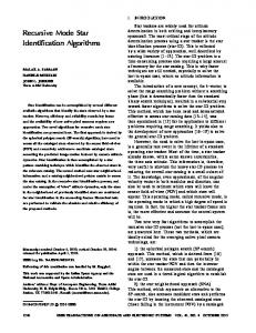
Fig. 2. Estimation of parameter at in case 1.

Fig. 1. Comparison of EMSE of the PR-RLS, BLRLS and SR-VFF-QRRLS algorithms.

The vector time-varying parameter process θt (k) is produced from a deterministic FIR filter θ0 (k) with tap length N as

1

κ

θ0 (k) =

N +1

   k,

1≤k
N

N +1

2

(37)

where κ is chosen such that ∞ 

|θ0 (k)|2 =

k=−∞

N 

|θ0 (k)|2 = 1.

k=1

The input sequence of this experiment is assumed as independent and identically distributed (i.i.d.) and normally distributed with variance σQ2 . The variance of the measurement noise is σ 2 and the different branches of system parameters are assumed uncorrelated thus the covariance matrix R = σR2 I. In this simulation the parameters are chosen as: N = 11, σQ2 =

1, σ 2 = 0.5, and σR2 = 8 × 10−4 . The signal to noise ratio (SNR), σ2

calculated as σQ2 , is 3 dB in this simulation. The parameter ρ is assigned as 0.9995. Fig. 1 shows the EMSE of the PR-RLS algorithm, the BLRLS algorithm and the SR-VFF-QRRLS algorithm. The result is an average of 100 Monte Carlo simulations. It is easy to observe that the PR-RLS algorithm can achieve lower EMSE than the other two algorithms. Additional experiments (not shown here to save space) have verified that the proposed PR-RLS algorithm tends to have good performance even under smaller SNR. In the second simulation, the sample time-varying system is described by (see also [19]) yt = at yt −1 − 0.45yt −2 + 0.1yt −3 + 0.3xt −1 − 1.5xt −2 + vt , where yt is the system output; xt is the system input with zero mean and unit variance; at is a time-varying parameter to be estimated and vt is the measurement noise with 0 mean and a variance of 0.001. Two cases were simulated to compare the performance of the algorithms: 0, 1,

 Case 1 : at =

sin(0.005t ) ≤ 0.5 , for others

Case 2 : at = sin(0.005t ). Case 1 checks the performance for non-persisting excitations and Case 2 examines the tracking ability of a periodic signal. Figs. 2 and 3 compare the estimations of at by the three algorithms together with the real value of at , in Cases 1 and 2,

Fig. 3. Estimation of parameter at in case 2.

respectively. The proposed PR-RLS algorithm can achieve better performance than the BLFRLS algorithm and the SR-VFF-QRRLS algorithm for tracking parameter at . Note that in this simulation, the parameter ρ is assigned as 0.9999. The third simulation compares the performances of the three algorithms using an identification problem with sudden changes. The channel coefficients are determined by

θt +1 = θt + ωt . The initial parameters satisfy

θ0 = [0.1, 0.2, 0.3, 0.4, 0.5, 0.6, 0.7, 0.8, 0.9, 1]T and there is a sudden change at the 300th iteration,

θ300 = [0.1, −0.2, −0.3, −0.4, −0.5, −0.6, 0.7, 0.8, 0.9, 1]T . The system parameters toggle between the two sets of parameters every 300 iterations. The ωt is a white Gaussian vector with variance matrix σR2 × I. Both the white input signal and colored input signal are used to excite the system under different SNRs. The colored input is simulated by a first-order autoregressive (AR) process: xt = 0.9xt −1 + vt , where vt is a zero mean Gaussian sequence with unit variance. The resultant EMSEs are obtained under 1000 Monte Carlo simulations. Fig. 4 shows the EMSE obtained by the three algorithms with white input, SNR being 20 dB and σR2 being 0.00005. The proposed PR-RLS algorithm can achieve lower EMSE than the SRVFF-QRRLS algorithm and the BLRLS algorithm. More importantly, the response of the PR-RLS algorithm is much faster than the SRVFF-QRRLS algorithm when the system parameters experience a sudden change. Note that in the third simulation, the parameter ρ is assigned as 0.9995.

J. Li et al. / Systems & Control Letters 66 (2014) 104–110

109

Fig. 4. Comparison of EMSE of the three algorithms under white input and low system noise.

Fig. 6. EMSE obtained the M-RLS algorithm and other algorithms.

Fig. 5. Comparison of EMSE of the three algorithms under colored input and high system noise.

Should the system parameter noise increase, the PR-RLS algorithm remains its good performance. Fig. 5 examines the EMSE with colored input, SNR being 20 dB and σR2 being 0.001. The PRRLS algorithm still maintains its performance of faster tracking and lower EMSE. 5.2. Simulation results for the M-RLS algorithm The fourth simulation reported in this sub-section shows the advantages of the proposed M-RLS algorithm. Here we assume that the different branches (tap length N = 11) of system parameters have different variances so that the matrix R is represented as R = diag{(5i × 10−5 )i=1,...,N }. Assume that the input sequence xt is produced by the following ARX(2,1) model: xt = 0.2xt −1 + 0.4xt −2 + 0.35vt −1 + vt , where vt is the driving noise with zero mean and unit variance. The resulting input sequence xt is correlated and the covariance matrix Q of the input vector is not a diagonal matrix. The true system parameters are initialized according to (37) and are propagated under random walk model. The measurement noise variance σ 2 is assumed to be 0.5. The optimal matrix forgetting factor F for the M-RLS algorithm can be calculated by (36). Obviously, the M-RLS algorithm can attain a smaller EMSE than the other scalar forgetting factor RLS algorithms since it exploits well the different changing rates of different system parameter branches. Fig. 6 compares the EMSE obtained by the M-RLS algorithm, the PR-RLS algorithm, the BLFRLS algorithm and the SR-VFF-QRRLS algorithm. It is observed that the M-RLS algorithm can achieve better performance than all the other three RLS algorithms. As the M-RLS algorithm is also implemented with regularization, another case of the fourth simulation demonstrates the performance of M-RLS algorithm with non-persisting excitation. We

Fig. 7. Parameter Estimation by M-RLS algorithm and other algorithms.

consider that the parameters experience sudden changes and become zero for some duration. The experimental setup is the same except that the true system parameter will abruptly change and the SNR is 10 dB. The parameters are initialized as in (37). The true parameter will toggle between two sets of parameters (the initial value and zero). Note that the parameter setting of this sub-case could be considered as a mixture of Case 1 of the second simulation and the third simulation. Between each toggling, the system parameters are modeled as random walk. Fig. 7 illustrates the estimations for one of the channel parameters by various algorithms. As shown, the M-RLS algorithm is performing well even with nonpersisting excitation. The main reason for the high performance of M-RLS is that it requires more information about the system noise and measurement noise to determine its matrix forgetting factor. If the system parameter variances are known a priori and the variances of different channels are not the same, it is much more advantageous to use the proposed M-RLS algorithm. 6. Conclusion A parallel self-tuning RLS algorithm with regularization (PRRLS) has been proposed which can automatically determine the desirable forgetting factor while performing recursive system identification. The EMSE of the incorporated regularization algorithm has been rigorously derived. Further, an RLS algorithm using matrix forgetting factor (M-RLS) has been presented which can provide optimal identification of parameter branches with different changing rates. The close form of the optimal matrix forgetting factor and the resulting EMSE of the M-RLS algorithm have also been discussed.

110

J. Li et al. / Systems & Control Letters 66 (2014) 104–110

Acknowledgments We would like to thank the reviewer and editor for the constructive comments and suggestions which helped improve the presentation of the paper. We wish to acknowledge the funding support for this project from Nanyang Technological University under the Undergraduate Research Experience on Campus (URECA) programme, and to thank Professor S.C. Chan for his kind help in providing the source code of the SR-VFF-QRRLS algorithm presented in [21]. References [1] L. Ljung, S. Gunnarsson, Adaptation and tracking in system identification — a survey, Automatica 26 (1) (1990) 7–21. [2] A.H. Sayed, N.J. Hoboken, Adaptive Filters, John, Wiley & Sons, Inc., 2008. [3] L. Ljung, T. Soderstrom, Theory and Practice of Recursive Identification, MIT Press, Cambridge, 1983. [4] Y. Zheng, Z. Lin, Recursive adaptive algorithms for fast and rapidly timevarying systems, IEEE Trans. Circuits Syst. II 50 (9) (2003) 602–614. [5] Q. Song, H. Chen, Identification of errors-in-variables systems with ARMA observation noises, Systems Control Lett. 57 (5) (2008) 420–424. [6] G. Li, C. Wen, Convergence of normalized iterative identification of Hammerstein systems, Systems Control Lett. 60 (11) (2011) 929–935. [7] M. Fu, Z. Deng, J. Zhang, Theory and its Application in Navigation System, Science Press, Beijing, 2003. [8] T.R. Fortescue, L.S. Kershenbaum, B.E. Ydstie, Implementation of self-tuning regulators with variable forgetting factor, Automatica 17 (6) (1981) 831–835. [9] S.D. Douglas, A. Antoniou, A parallel adaptation algorithm for recursive-leastsquares adaptive filters in nonstationary environments, IEEE Trans. Signal Process. 43 (11) (1995) 2484–2485. [10] S. Song, J.S. Lim, S. Baek, K.M. Sung, Gauss Newton variable forgetting factor recursive least squares for time varying parameter tracking, Electron. Lett. 36 (11) (2000) 988–990. [11] S. Leung, C.F. So, Gradient-based variable forgetting factor RLS algorithm in time-varying environments, IEEE Trans. Signal Process. 53 (8) (2005) 3141–3150. [12] C. Paleologu, J. Benesty, S. Ciochina, A robust variable forgetting factor recursive least-squares algorithm for system identification, IEEE Signal Process. Lett. 15 (2008) 597–600.

[13] J. Wang, A variable forgetting factor RLS adaptive filtering algorithm, in: Proceeding of the 3rd IEEE International Symposium on Microwave, Antenna, Propagation and EMC Technologies for Wireless Communications, 2009, pp. 1127–1130. [14] S. Ciochina, C. Paleologu, J. Benesty, A.A. Enescu, On the influence of the forgetting factor of the RLS adaptive filter in system identification, in: Proceeding of the International Symposium on Signals, Circuits and Systems, 2009, pp. 1–4. [15] F. Ding, T. Chen, Performance bounds of forgetting factor least-squares algorithms for time-varying systems with finite measurement data, IEEE Trans. Circuits Syst. I. Regul. Pap. 52 (3) (2005) 555–566. [16] L. Ljung, Recursive least-squares and accelerated convergence in stochastic approximation schemes, Internat. J. Adapt. Control Signal Process. 15 (2) (2001) 169–178. [17] A. Ali, A.U. Rehman, R.L. Ali, An improved gain vector to enhance convergence characteristics of recursive least squares algorithm, Int. J. Hybrid Inf. Technol. 4 (2) (2011). [18] M.Z.A. Bhotto, A. Antoniou, Robust recursive least-squares adaptive-filtering algorithm for impulsive-noise environments, IEEE Signal Process. Lett. 18 (3) (2011) 185–188. [19] W. Yu, N. Shih, Bi-loop recursive least squares algorithm with forgetting factors, IEEE Signal Process. Lett. 13 (8) (2006) 505–508. [20] R. Arablouei, K. Dogancay, Modified RLS algorithm with enhanced tracking capability for MIMO channel estimation, Electron. Lett. 47 (19) (2011) 1101–1103. [21] S.C. Chan, Y.J. Chu, A new state-regularized QRRLS algorithm with a variable forgetting factor, IEEE Trans. Circuits Syst. II: Express Briefs 59 (3) (2012) 183–187. [22] M.Z.A. Bhotto, A. Antoniou, New improved recursive least-squares adaptivefiltering algorithms, IEEE Trans. Circuits Syst. I. Regul. Pap. (2013). Published online. [23] F. Ding, H. Yang, F. Liu, Performance analysis of stochastic gradient algorithms under weak conditions, Sci. China F: Inf. Sci. 51 (9) (2008) 1269–1280. [24] J. Zhang, F. Ding, S. Yang, Self-tuning control based on multi-innovation stochastic gradient parameter estimation, Systems Control Lett. 58 (1) (2009) 69–75. [25] A.S. Poznyak, J.J. Medel Juarez, Matrix forgetting factor, Int. J. Syst. Sci. 30 (2) (1999) 165–174. [26] A.S. Poznyak, J.J. Medel Juarez, Matrix forgetting factor with adaptation, Int. J. Syst. Sci. 30 (8) (1999) 865–878. [27] S. Gunnarsson, Combining tracking and regularization in recursive least squares identification, in: Proceeding of the 35th IEEE Conference on Decision and Control, Vol. 3, 1996, pp. 2551–2552.