Recursive Identification Algorithms for Right Matrix Fraction ...

AUTOMATIC TRANSACTIONS ON

NO. CONTROL, AC-29, VOL.

REFERENCES A. Bensoussan and J. L.Lions, Applications des iniquations variationnellesen contrbe stochastique, Dunod, 1978. I. B. Rhodes, “Recursive state estimation for a setD.P.Bertsekasand membership description of uncertainty,’’ IEEE Trans. Automat. Contr., vol. AC-16, Apr. 1971. J. M. Bismut, “An example of optimalcontrolwith constraints,” SIAM J. Contr., vol. 12, no. 3, pp. 4 0 4 1 8 , 1974. -, “Linear quadratic optimal stochastic control with random coefficients,” SIAM J. Contr. Optimiz., vol. 14, no. 3, pp. 419-444, 1976. N. Christopeit, “A stochastic control model with chance constraints,” SIAM J. Contr. Optimiz., vol. 16, no. 5 , pp. 702-714, 1978. E. A. Coddington and N. Levinson, Theory of Ordinary Differential Equalions. New York: McCraw-Hill, 1955. M. H. A. Davis, Linear Estimation and Stochastic Control. London: Chapman and Hall, 1977. L. D. Edinger, G.B. Skelton, C. R. Stone, M. D. Ward, and G.D. White, “Final technical report: Designofload relief control system,’’ Syst. andResearch Division, Rapport Honeywell Inc., NASA Contract 8-20 155. W. H. Fleming and R. W. Rishel, DeterministicandStochastic Optimal Control. New York: Springer-Verlag, 1975. E. B. Frid, “On optimal strategies in control problems with constraints,” Theory Prob. Appl., vol. XVII. no. 1, pp. 188-192, 1972. U. G. Haussmann, “Some exampleofoptimal stochastic controls or: The stochastic maximum principle at work,” SIAMRev., vol. 23, pp. 292-307,1981, D. P. Kennedy, “On a constrained optimal stopping problem,” J. Appl. Prob., vol. 19, pp. 631-642, 1982. H. J. Kushner, “On the stochastic maximum principle with average constraints,” J. Moth. Anal. Appl., vol. 12, pp.13-26, 1965. M. K. Ozgoren, R. W. Longman, and C. A. Cooper, “Probabilistic inequality constraints in stochastic optimal control theory,” J. Math. Anal. Appl., vol. 66, pp.237-259,1978 M. Pontier and I. Szpirglas, “Arrzt optimal avec contrainte,” Advances Appl. Prob., Dec. 1983. M.Robin, “On optimal stochastic control problems with constraints,” in Game Theory andRelated Topics. Amsterdam, TheNetherlands:North-Holland, 1979, pp. 181-202. R. T. Rockafellar, Convex Analysis. E n g l e w d Cliffs, NJ: Princeton University Press, 1970. A. N. Shiryayev, “Optimal stopping rules.” Appl. Math., Springer-Verlag. 1977.

Recursive Identification Algorithms for Right Matrix Fraction Description Models

ARYE NEHORAI AND MARTIN M O W Abstract-Multivariable identification algorithms are usually designed only for left matrix fraction description 0 ) models. In this paperwe considerrecursive identification algorithms for rightmatrix fraction description (RMFD) models with diagonal denominator matrices. The algorithms are of prediclion error (PE)and model reference (MR) type. Results from simulations illustrate the performance of the algorithms. I. INTRODUCTION

Over the last few years, various algorithms have been suggested for online identification of multivariable system transfer functions. A general multivariable linear finite order discrete time system can be modeled by the input-output relationship Y ( 0 = M q - I)u(t)+ 40

1103

12, 1984 DECEMBER

(1)

where y ( t ) is the p-dimensional outputvector at time t , u(t) the rnManuscript received January 14, 1983. Paper recommended by C. R. Johnson, Jr., Past Chairman of the Identification Committee. This work was supported bythe Defense Research Projects Agency under Contracts MDA903-80-C-0331andMDA903-82-K0382, and in part by theJoint Services Electronics Program d e r Contract DAAG29-79c-0047. A. Nehorai \*as with the Information Systems Laboratory, Department of Electrical Engineering, Stanford University, Stanford, CA 94305. He is now with Systems Control Technology, Inc., Palo Alto, CA 94304. M. Morf waswith the Information Systems Laboratory, Department of Elecaical Engineering, Stanford University, Stanford, CA 94305. He is now with E.T.H. Institut fur Infonnatik, Zurich, Swiarland.

dimensional input, u ( t ) is the disturbance noise, and H ( q - ’ ) denotes the system transfer functionmatrix.Theelementsof H ( q - ’ ) are rational functions of the unit delay operationq - l , i.e., q - ’ u ( t ) = u(t - I), etc. Available mutivariable identification algorithms are usually designed only for left matrix fraction description (LMFD) models, Le., for y(t)=A-’(q-’)B(q-’)u(t)+u(t)

(2)

where A ( q - I ) and B ( q - ’ ) are p X p and p X m polynomial matrices, respectively, see, e.g., [1]-[6]. However, inmany practicalsituations in control, plantmonitoring, radar, and others, the model (2) maynot describe directly the desired physicalmechanisminsidethesystem. Consider, for instance, a plant whose inputs undergo local processes of autoregressive ( A R ) type and then they are superimposed by a global moving average (MA) process (typically, weighted delay or multipath in a medium). This description corresponds to the right MFD (RMFD)model y(t)=C(q-’)D-’(q-‘)u(t)+u(t)

(3)

where the polynomial matrixC(q- I) is p X rn and D(q - I ) is an rn x rn diagonal matrix. The input-output relationship of this model, which shall be called the DRMFD for the diagonal denominatorRMFD, is illustrated in Fig. 1. In this paper we shall derive recursive identification algorithmsfor the DRMFD model (3) shown in Fig. 1.The algorithms will be of prediction error (PE) type developed by Ljung [T, [8], and of output error model reference (MR) designed byLandau [3], [9]. They will be particularly advantageous in situations where the DRMFD of the true system is such thattheelementalsubsystems c${q-’)/d$q-’) are minimal. (The superscript o denotes the true system.) We should remark that an alternative way to estimate the DRMFD model (3) would be to firstapply LMFD algorithmsandthenapply tranformations from LMFD to RMFD forms. However, this approach would suffer from two maindisadvantages,especiallywhen the true system has aminimal DRMFD in the above sense. Thefirst disadvantage it too high a load of computations, due to the overparametrization inthe model as well as the need of transformation; the second disadvantage is inaccuracy due to the use of an inappropriate model. Anotherapproach for estimating the model (3) usingavailable algorithmswouldbe to apply the instrumentalvariable (TV) type algorithm of [lo] designed for the multiinput single-output case of the model (3) by estimatingthecorresponding transfer functionentry by entry. This method cannot be applied to all inputs and outputs together. For themultioutput case, the samedenominatorsassociated with the inputs would have to be separately estimatedfor each output as different polynomials. In general, the ineffectiveness of available algorithms for the DRMFD systems is due to the fact that they are not constrained to the special form of (3). The main difficulty in deriving algorithms for the RMFO model (3) stems from the fact that one cannot eliminate the inverse D-’(q- I) by premultiplying (3) by D ( q - ’ ) . Todemonstratetheusefulnessofthemodel (3), wemention two practical examples of this form. The first one is the DRMFD modelof the power system consideredby Sinha and Caines[l 11. The other exampleis the multivariable rational model of signals received in distributed array of sensors from multiple distant sources of energy waves; see [12]-[14]. This scenario often occurs in radar, seismology, and astronomy. The convergence of the RMFD output error MR algorithm below is analyzed in[131 using theordinary differential equation (ODE) method of Ljung [15]. The results give thepositiverealnesscondition for its convergence to the true RMFD of the system. This condition generalizes the scalar case in [13]. The RMFD PE schemeconverges to alocal minimum of the criterion w.p.1 by the general resultsof the PE family of algorithms [T. II. THE RMFD A L G O R I T H M S

The Basic Assumptions 1) The true system transfer function H o ( q - ’ )is strictly proper, stable, and with monic denominators. 2) The stochastic processes u(t) and v ( t )

0018-9286/84/1200-1103$01.00 01984 IEEE

1104

IFEE TRANSACTIONS ON AUTOMATIC CONTROL, VOL. AC-29, NO. 12, DECEMBER 1984

Fig. 1. Schematic description of the DRMFD model.

are stationarywithrationalspectraldensitiesandsuchthat all their moments exist (note, they can also have deterministic components). 3) The system operates in open loop and/or the noise u ( t ) is white. 4) The input u ( f ) isuncorrelatedwith u(t). 5) Thedifferentinputs are uncorrelated. 6) The order of the algorithm is not smaller than the true system order. These assumptions were used in the convergence analysis of [13]. Notice that we have not included an elemental minimality assumption on the DRh4FD of the true system. The reason for this is that when this description is nonminimal, thealgorithmsbelow can still yieldan estimated transfer function which givesthe true input-output relations for all nonminimal subsystems; see [13].

(13a) e=[(ed)Ti

(e;)', ..., ( s ; ) ~ ](~n , + p - n , ) . m x l .

The Gradient Matrix

For the derivation of the recursive PE algorithm [7l, [SI we need also the gradient matrix

w , e)=The Prediction Signal

To derive the regression expression for the predicted output vector, note from (3) that

(13b)

The special structure of + ( t , 8) and 6 reflects the particular form of the DRMFD model (3).

d5'(t, 0) dB

.

(14)

From (4) it is easy to check that the entries of this matrix are given here by V A t , 6) Cu(q-9 1 -- -u,(t-k)= -yu(t-k, adjk +-'I d,(q-')

e)

(15a)

so that with the assumption of uncorrelated inputs we may write This implies that$( r, 0) has here the same formas $(t, 0). except for the prefiltering of 9&, 0) and uJt) by l/d'q-I).

where 8 denotes the unknown system parameter vector and c d q - I) j o ( t , e) = -uj(t). djd-l)

(6)

For notational convenience,we shall restrict ourselves to the special case where the orders of the polynomials c& - I) are all equal to n,, and the orders of dj(q - I ) eqwd to nd. Equation (6) can be rewritten equivalently as

update $(t)- >$(t+ (16W 1) j(t+

l)=+T(t+ I)@).

(16i)

The weighting sequence X(t) is updated in the stationary case by h(t) = &X(t - 1) + (1 - &) where typically X, = 0.99 and X(0) = 0.95. The variable y ( t ) is updatedby y(t) = y ( t - l)/[y(t - 1) + h(r)]. The

' Notice that d&, 8) and 8" defined earlier are not the ijtb entries of + ( f ,

8) and 8.

1105

0.5

0.0

-0.5

-1.0

1.5

1.5

1.0

1.0

42 0.5

ClZl

5 1 1 0.5

du

cuz

0.a

0.0 %l

cu2

cm -0.5

-0.5

czu -1.0

-1.0

-1.5

-1.5 0

Ya

lm,

1 m

zwo

TLIZ

(4

o

m

1mO

15Ol

TllL

(d)

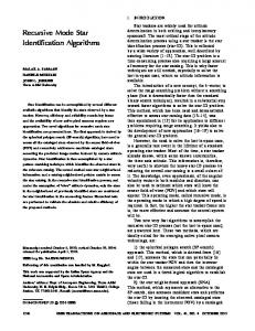
Fig. 2. Parameter estimates with their true values for the 2 x 2 second-order system of Section III using the recursive RMFD algorithms. S N R (i,j ) = 0 dB. (a) coefficientscorresponding to input 1. @) MR, coefficients corresponding to input 2. (c) PE, coefficients corresponding to input 1. (d) PE, coefficients componding to input 2.

MR.

above recursions are applicable to our case with the distinction thatd ( f ) and $(t) have the special forms describedin (615) for d(t, 0) and $(t. 0) with 0 replaced by ^e(t);see also [13].

d,"(q-')= 1 +0.25q-'+0.70q-2

Output Error MR Algorithm

The output error MFi algorithm is based on the assumption of linearity of the regression equation (12) in the model0, which implies that it can be found by replacing $(t) with 4(t)above. Refiltering of the output error MR algorithm can be performed to avoid the positive realness condition required for the convergence, as was suggested by Landau [3], [17];see 'also [16] and [18]. For the various possible prefilteringsin our case, see ~31. We usethe methods of SectionII with the assumption of known orders. Initializations usedare P(0) = lOO&,A(0) = Z2,and e(0) = 0. From the convergenceanalysis of 1131 we expectthealgorithmstoconverge The system to be identified is as in (3) with two-inputs, two-outputs, asymptotically w.p.1 to the true system parameters. and second-order polynomials. The input signal u(t) and the noiseu ( t ) are Fig. 2 illustrates the results of the RMFD algorithms for the above white,normallydistributed,with zero mean, andidentity covafiane system. Fig. 2(a) and (b) shows the estimated coefficients computed by matrix. (Note that the above algorithmsare equally applicable for Inputs the RMFD MR algorithm (without prefiltering)as a function of time,for and noise of ARMA type, with or without deterministic components.) the tirst and secondinput, respectively. The straight lines denote the true c;(q-') are scaled to give the desired signal-to-noise ratio S N R ( i , J ] = 0 values.Theseparationintodifferentinputparameterswasdonefor dB between the power of the ijth noiseless subsystem output and the noiseconvenience of presentation. Fig. 2(c) and (d) shows theanalogous results power at the ith output. The true system polynomialsare: from the RMFD PE algorithm. The simulation results show in general thatthe estimates approach their true value after several hundred time samples. In [13] we present a first-

III. SIMULATION E W L E S

1106

IEEE TRANSACTIONS ON AUTOMATIC CONTROL, VOL. AC-29, NO. 12, DECEMBER 1984

order example. The convergence rate was usually faster for first-order systems than for second order; see also [19] for similar results in the in the scalar case. Note also that there is nosignificantdifference convergencerateandaccuracybetween the denominatorandthe numerator estimates. The convergence .ratecan be improved by using a recursive-itemtive algorithm; see, e.g., [5], [IO].

N.CONCLUSION We have presentedrecursive identification algorithmsof PE and output error MR type for the RMFD model (3), which is different from LMFD models commonly used in system identification. Some possible extensions for more gene@ modeling and IV schemes are discussed in [13]. Inclusion estimation of the noise model can improve the accuracy of the results butwouldrequiremorecomputationsand decreasetherobustness of thealgorithm with respecttothenoise properties. Other modificationsto unknown inputs are particularly useful for on-linelocalizationandidentification of multipledistantradiating sources from signalsreceivedinadismbutedarray ofpassive radar sensors. This modificationcan be doneby using pasterrors as estimatesof the inputs. The close relation between theRMFD model and the controller canonical form (see, e.g., [20])suggeststhatmoreresearch onthe recursive RMFD identification will be useful for adaptive control.

REFERENCES

R. Guidorzi, “Canonical structures in the identificationof multivariable systems,” Automafica, vol. 11, pp. 361-374,1975. R. L.Kashyapand A. R. Rao, Dynamic Stochastic Models from Empirical Data. NewYork:Academic, 1976. I. D. Landau, “Unbiased m i v e identification using model reference adaptive techniques,” IEEE Trans. Automat. Contr., vol. AC-21, pp. 194-202,1976. L. Ljung, “Convergence of an adpative filter algorithms,” Int. J . Contr., vol. 27, no. 5, pp. 673493, 1978. methods of A. J. Jakemanand P. C. Young,“Refinedinstrumentalvariable recursive time-series analysis, Part II: Multivariable systems,” Inf. J. Contr., vol. 29, pp. 621644, 1979. P. Stoicaand T. Saderstrom, “Identification ofmultivariable systems using instrumental variables methods,” 1981. L. Ljung, “Analysis of a general recursive prediction ermr identification algonthm,” Automatica, vol. 17, no. 1. pp. 88-99, 1981. L. Ljungand T. Siidersaiim, Ttieoty and Practice of Recursive Identificotion. Cambridge, MA: M.I.T. Press, 1983. I. D. Landau, “A survey of model reference adaptive techniques-Theory and applications” Aufomafica, vol. 10, pp. 353-379, 1974. A. J. Jakeman, L. P. Steele, and P. C. Young, “Instrumental variable algorithms for multiple input systemsdescribed by multiple transfer functions.” IEEE Trans. Syst. Man. Cybern., vol. SMC-IO, pp. 593-€02, Oct. 1980. S. Sinha and P.E. Caines, “On the use of shifi register sequences as insmental variables for the recursive identificationof multivariable l i n e a r systems,” Int. J. Syst. Sci., vol. 8. pp. 1041-1055,1977. M. Morfet al.,Technical Summary Report to DARPA, SEL Rep. M355-1. Mar. 1979. A. Nehorai, “Algorithms for system identification and source locabion,” Ph.D. dissertation, Dep. Hec. Eng., Stanford Univ., Stanford, CA, June 1983. A. Nehorai, G. Su, and M. Morf. “Estimation of time differences of arrival by

pole decomposition,” IEEE Trans. Acoust., Speech, Signal Processing, vol. ASSPJI, no. 6, pp. 1478-1492, DE. 1983. L. Ljung, “Analysis of recursive stochastic algorithms,” IEEE Trans.Automat. Contr., vol. AC-22, pp. 551-575, Aug. 1977. L. Ljung, “On positive real transfer functions and the convergence of some recursive schemes,” IEEE Trans. Automat. Contr., vol. AC-22, pp. 539-551, Aug. 1977. I. D. Landau, “Elimination of thereal positivity condition in the design of @el MRAS,” IEEETrans. Automat. Confr., vol. AC-23, pp. 1015-1020, Dec.

Model Updating Improves MRAC Performance P. P. J.

VANDEN BOSCH AND P. I. TJAHJADI

Abstract-The performance of an MRAC design can be improved by using the model-updating concept, which places the state of the system into the reference model at regular time intervals. This paper discnsses criteria for determining this updating and a proof is given to show that model updating does not influence the stability properties of an MRAC design. A typicalexampleindicates an improvement in the control performance obtained by the application of model npdating. INTRODUCTION

Model-reference adaptive control (MRAC) is a well-established design method that has demonstrated its capabilities in many interesting applications; for example [I]-[3]. Asymptotic stabilitycan be proved for linear systems.Even for nonlinearsystems,stabilityandagood performance can be obtained. Model updating can improve the performance of an MRAC design, in particular for systems whose structure does not match the structure of their reference model. Suppose that the state y of the system differs from the state x of the reference model. Then, via an adjustment of the controller parameters, MRAC w l i force thesystemtofollowthe reference model.Ifthe structure of the system and that of the reference model differ, there is no unique parameter set for the controller that is able to realize a zero error between the state y of the system and thestate x of the reference model. Consequently, oscillations ofy about x can be expected, as illustrated in Fig. 1. The philosophyof modelupdating is to reduce these oscillations. Model updating replaces thestate of thereference model bythe actual state of the system at some points in time. Ultimately, there is no difference between y and x, and thus there are no parameter adjustments. New reference trajectories are calculated, starting in theactual state ofthesystem. Therefore, modelupdatingavoids unnecessary control efforts and anticipates disturbances better. In this paper we will discuss criteria for determining an appropriate point in time in which to apply model updating and we will prove that model updating does not influence the asymptotic stability of an MRAC design. Results of a feasibility study, concerning a three-axes slew for satellites, illustrate the improvements of model updating over a standard MRAC design. UPDATE

CRITERIA

Landau [l] has proposed an update at each sample time ofMRAC for discrete systems. In that case, we have the series-parallel structure of MRAC. Continuous systems require a differentapproach. In [4] we used a fixed value for the update interval. Every Tup seconds the state of the system was introduced intothe reference model. The choiceof this fixed interval turned out to be critical. Now we willpropose acriterion based on the Lyapunov functionV.In an MRAC design this function consistsof an expression dealing with the error e(e = x - y ) and an expression dealing with the differencep between the parameters of the reference model and those of the system, so V(e,p)=e’Pe+ V(p).

If we use appropriate adaptive laws, we obtain [l] V(e)= - e ’ Qe

1978.

P. Young, “Some observations on instrumental variable methods of time-series analysis,” Inf. J. Contr., vol. 23, no. 5. pp. 593-612, 1976. T. Sidersuom, L. Ljung.and I. Gustavson, Dep. Automat. Conrr., Lund Inst. Technol., Lund, Sweden, Rep. 7427, 1974. T. Kailath, Linear Systems. E n g l e w d Cliffs, NJ: Prentice-Hall, 1980.

Manuscriptreceived August 12, 1983; revised December 6, 1983 and March27, 1984. The authors are with the Laboratory for Control Engineering, Delft Universityof Technology, Delft, The Netherlands.

0018-9286/84/1200-1106$01.00 0 1984 IEEE