Recycling Data for Multi-Agent Learning
Santiago Onta˜ n´ on Enric Plaza IIIA, Artificial Intelligence Research Institute, CSIC, Spanish Council for Scientific Research. Campus UAB, 08193 Bellaterra, Catalonia (Spain).
Abstract Learning agents can improve performance cooperating with other agents, particularly learning agents forming a committee outperform individual agents. This “ensemble effect” is well known for multi-classifier systems in Machine Learning. However, multiclassifier systems assume all data is known to all classifiers while we focus on agents that learn from cases (examples) that are owned and stored individually. In this article we focus on how individual agents can engage in bargaining activities that improve the performance of both individual agents and the committee. The agents are capable of self-evaluation and determining that some data used for learning is unnecessary. This “refuse” data can then be exploited by other agents that might found some part of it profitable to improve their performance. The experiments we performed show that this approach improves both individual and committee performance and we analyze how these results in terms of the “ensemble effect”.
1. Motivation: Embracing Distributed Data Distributed data mining and knowledge discovery accepts the fact that some data are and will continue to be essentially decentralized. Currently, the focus is on incremental but centralized techniques capable of working with distributed data. Our approach, however, focuses on decentralizing the process of learning and knowledge discovery as well. In the framework of multi-agent systems, individual agents are not Appearing in Proceedings of the 22 nd International Conference on Machine Learning, Bonn, Germany, 2005. Copyright 2005 by the author(s)/owner(s).
[email protected] [email protected]
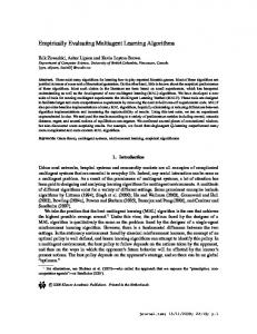
merely repositories of knowledge, but active components capable of problem solving and learning (from their own data and possibly from data exchanged with other agents). A related notion to distributed data is ensemble learning, that is to say working with multiple learning models of data. These approaches study the advantages of having more than one set of data and/or more than one model of learning from data. The most common way to describe ensemble learning is that, rather than building a single predictive model, a collection (or ensemble) of models is built and their predictions are then efficiently combined (e.g. by voting). There are different ways to achieve ensemble learning but they always have to achieve the same property: that the error of multiple learning models is not correlated. Essentially, the ensemble effect amounts to the fact that combining multiple predictions (such that predictors are minimally competent and their errors are not correlated) is better than any individual predictor. Figure 1 shows two ways of achieving the ensemble effect: (a) methods that transform a data set D into a collection of data sets and (b) methods that use different learning techniques upon the same data set D. Two examples of (a) are bagging (Breiman, 1996) (a method to create multiple subsets of D such that error correlation is lowered) and feature subsets (Bay, 1998) (a method to select different subsets of features representing data and thus constructing a collection); both are ways to achieve error de-correlation from an original set of data. Finally, (b) uses multiple classifiers built with different ML techniques that in this way insure their errors are not correlated. The rationale of ensemble learning is thus that having multiple data sets is, under certain conditions, even better than having a single data set. On the other hand, we have seen that data is inherently distributed in real-life applications, so having multiple data sets is a fact of life; there is no security however that they
Recycling Data for Multi-Agent Learning
Solution
(a)
D D1 D2 D3 D4 D5 Solution
D
M1
M2
M3
M4
(b)
Figure 1. Two forms of forcing the ensemble effect by decorrelating multiple classifiers.
comply to the conditions needed for having the benefits of the ensemble effect. Our research focuses on developing techniques that embracing the fact that data is distributed are able to achieve (distributed) data sets that comply to the conditions required by the ensemble effect. Moreover, we focus on multi-agent techniques to achieve this goal, in such a way that the autonomy of decision concerning the data accessed, shared or exchanged, is always in the hands of individual agents (and not some centralized process that simply accesses remote data repositories). Finally, notice that most ensemble learning techniques assume a centralized approach in that all data is available to a central process that later decides unilaterally how it is distributed. Recent work has proposed multi-agent techniques for achieving comparable or even better performances than a centralized approach (Onta˜ n´ on & Plaza, 2001). In this paper we present a new technique to redistribute data among individual agents in order to achieve data sets that exhibit the ensemble effect.
2. Waste economy and recycling To understand the data redistribution technique we will propose it is useful to consider the metaphor of recycling in an economy of refuse materials (wastes). Figure 2 shows on the left a firm FIRM that consumes input material and outputs both product and refuse materials (shown in three colors in the example). Now, waste economy is based on the fact that most refuse can be reused as input for other firms (possibly after some pre-processing) in the industrial ecology. The refuse market of Fig. 2 is a decentralized mechanism for coordinating the needs of different firms to acquire input materials and the needs of other firms to get rid
of refuse materials. The firms offer in the refuse market those refuse materials they produce and acquire input materials that the can use (possibly after some preprocessing). The intended effect is clearly the efficient recycling of of most industrial by-products. We will present a data redistribution technique based on this idea of refuse recycling, although we will use a simple bargain model that will not require a monetary economy. Let us first consider the notion of refuse in the context of systems that learn from data. Currently, machine learning and data mining researchers have realized that the intuitive idea that “the more data the better learning” is not true. In fact, the selection of the data that should be fed to a particular ML technique is itself a constituent part of the data mining process. Moreover, any specific ML technique treats data in a specific way that makes that some part of the data may not be useful to improve the overall performance. For instance, bagging (Breiman, 1996) builds multiple subsets of data, that is to say eliminates some part of the data for any particular data set generated. In the context of case-based reasoning and learning (CBR), retaining every known case may often degrade the performance of the CBR system (Smyth, 1996; Arcos, 2003). Case base maintenance is needed in order to decide which cases are retained (to learn from them) and which should be considered refuse (in order to improve the learning performance). In the context of multi-agent systems, where each agent is capable of learning from data to perform some individual prediction, the existence of refuse data together with their autonomy requires the agents to be capable of self-evaluating their own performance. Once an agent has this capability it can autonomously decide which data is refuse and, from that moment, cooperate with other agents in a process of exchanging refuse data. For this second purpose an agent will clearly need a technique to evaluate the data refused by others in order to decide which data is interesting (or to which degree it is interesting for him to acquire each datum). Once we have these two individual decision policies the third element needed is a market-like bargaining process that allocates the (refuse) data to that agent that is more interested. These three elements are the building blocks of the data recycling technique for multi-agent learning that we present in the following sections. The paper is organized as follows: Section 3 presents the multi-agent framework used in our work and the Committee Collaboration Strategy that the agents use in order to act as an ensemble, while Section 4 presents the Recycling Collaboration Strategy including both
Recycling Data for Multi-Agent Learning
FIRM
PRODUCT
FIRM_2
PRODUCT
REFUSE REFUSE
REFUSE MARKET FIRM_3
PRODUCT REFUSE
Figure 2. Waste economy based on a refuse market.
the interaction protocol and the individual decision policies that the agents need in order to implement a refuse bargaining strategy with the cases in their individual case bases. Finally, Section 5 presents an experimental evaluation of the Recycling Collaboration Strategy, and the paper closes with future work and conclusions sections.
3. Multi-agent CBR Systems A multi-agent CBR (MAC) system M = {(Ai , Ci )}i=1...n is composed on n agents, where each agent Ai has a case base Ci . A case base Ci = {(Pj , SPj )}j=1...N is a collection of problem/solution pairs. In the experiments reported here we assume that initially case bases are disjunct (∀Ai , Aj ∈ M : Ci ∩ Cj = ∅), i.e. initially there is no case shared by two agent’s case bases. In this framework we restrict ourselves to analytical tasks, i.e. tasks (like classification) where the solution is achieved by selecting from an enumerated set of solutions S = {S1 . . . SK }. Agents in a MAC system can solve problems individually by using its individual case base, but can also collaborate with other agents in order to solve a problem. In our framework, all the interaction among agents is performed by means of collaboration strategies. Definition 3.1 A collaboration strategy hI, D1 , ..., Dm i defines the way in which a group of agents inside a MAC collaborate in order to achieve a common goal and is composed of two parts: • an interaction protocol I, • a set of individual decision policies {D1 , ..., Dm }. The interaction protocol of a collaboration strategy de-
fines a set of interaction states, a set of agent roles, and the set of actions that each agent can perform in each interaction state. Each agent use its individual decision policies to decide which action to perform, from the set of possible actions, in each interaction state. When a group of agents solve a problem together they act as a committee: each individual agent solves the problem independently, and then they aggregate the individual solutions using a voting system. Specifically, the committee collaboration strategy can be summarized as follows: when an agent Ac is interested in solving a problem P in a collaborative way, Ac convenes a committee of agents Ac that contains agents willing to collaborate in solving P . Then, Ac sends the problem P to all the other agents in the committee. Each agent individually solves the problem using the cases in their individual case bases and communicate their individual predictions to the convener agent Ac . Finally, the convener agent aggregates all the individual predictions using a voting system. Thus, acting as an ensemble. In our experiments we used BWAV (Bounded Weighted Approval Voting) (Onta˜ n´on & Plaza, 2001) as the voting system. The main idea is that each agent votes for solution classes depending on the number of retrieved cases for each class. Each agent has 1 vote that can be fractionally assigned to several solution classes; the larger the number of retrieved cases endorsing a solution class, the stronger an agent will vote for that class.
4. Case Recycling in Multi-Agent Systems In this section we are going to present the Recycling Collaboration Strategy (RCS) that allows a committee of agents to preform recycling of the cases in their
Recycling Data for Multi-Agent Learning
individual case bases. In general not all cases in the case base of a CBR agent are useful: some of them could have been useful in the past but become not useful because further cases have been retained, or simply older cases may become obsolete as time passes for the specific task that the CBR agent must perform. The idea of RCS is that every agent Ai in a MAC system selects a set of refused from its case base. We can define the cases CiR ⊆ Ci S refuse set C R = i=1...n CiR as the set of all the refused cases by the agents in a MAC system. Once every agent has selected its cases to refuse, a bargaining may take place where all the agents are able to make bids in order to retain individually interesting cases refused by other agents (since a case refused by an agent may be useful for another agent). Bids are exchanged using bid records. A bid record B = hA, c, bi is a tuple where A is the agent, c is the case and b is the bid value (that is a real number in the interval [0, 1]). Bargaining consists of a series of rounds and at each round every agent casts a bid for each case in the refuse set. The agent that has cast the highest bid retains the case c for which that bid was made. Then, c is removed from the refuse set C R and a new round starts. The bargaining ends when all cases in the refuse set have been retained or when no agent is interested in any of the remaining cases. Specifically, RCS can be defined as follows: Definition 4.1 The Recycle Collaboration Strategy (RCS) is a collaboration strategy hIRCS , DR , DB i, where IRCS is the RCS interaction protocol, DR is the Refuse Decision Policy that agents use to decide which cases they refuse, and DB is the Bidding Decision Policy, that agents use to make bids for the refused cases. In the remaining of this section we will present both the RCS protocol and the individual decision policies that the agents need to use for engaging in RCS.
broadcasts the parameter tb to the rest of the agents, that specifies the amount of time that the agents have to make bids for the cases during the case bargaining. 2. When an agent Aj receives the parameter tb , Aj uses its individual Refuse Decision Policy DR to select a set of cases CjR that is sent to the convener agent. When the convener Ac receives the refused cases of the rest of agents and has computed its own set of refused cases, Ac builds the refuse set C0R , and sends it to the other agents. 3. From the moment that Ac sends C0R to the rest of agents, each agent Aj is free to send a set of bid records Bj,t to the convener agent Ac . 4. Once the time tb is reached, no more bids are accepted. The convener agent looks for the bid record Bt = hA, c, bi with the highest bid Bt .b among all received bids (ties are solved randomly). Now, two situations may arise: • If Bt .b > 0, then, case Bt .c is removed from the refuse set, the winning bid is broadcast to the rest of the agents and the protocol moves again to step 3 where the agents will again be allowed to make bids for the remaining cases in the refuse set. • If Bt .b = 0 or the refuse set is empty, then either no agent is interested in any case or there are no more cases to be bargained. Then, the convener agent will sent a termination message to the rest of the agents and the protocol ends. The remaining cases in the refuse set are discarded. In the next sections the individual decision policies needed to use RCS are presented. 4.2. The RCS Refuse Decision Policy
4.1. The RCS Interaction Protocol In the RCS interaction protocol IRCS an agent will take the role of the convener agent Ac . Then, the convener agent sends the initial message to start the protocol, receives the refused cases and the bids from the other agents, and determines the highest bid. However, the convener agent has no special privileges over the rest of the agents during the case recycling process. IRCS is an iterative protocol based on rounds. We will use t to denote the current round; initially t = 0. Specifically, the IRCS protocol works as follows: 1. The protocol starts when the convener agent Ac
In order to engage in RCS, individual agents must be able to self-evaluate and detect if some of the cases they have used for learning are unnecessary. The cases considered unnecessary are refused and deleted from the agents’ case bases. The Refuse Decision Policy DR is used by the agents to decide which cases to refuse and which cases to retain. In this section we propose a refuse decision policy based on JUST (Onta˜ n´on & Plaza, 2004b) (JUstification-based Selection of Training Examples), that has been experimentally shown to be a sound technique for assessing the utility of having (or not having) a case in a case base.
Recycling Data for Multi-Agent Learning
JUST is a technique based in the notion of justifications that given a case base C obtains a reduced case base C r ⊆ C that at least has the same expected classification accuracy than C. The cases not selected by JUST are refused. A justification J built by an agent to solve a problem P that has been classified into a solution class Sk is a description of the relevant information of P used for predicting Sk as the solution class, and can have many uses in multi-agent and CBR systems. Specifically, justifications in JUST are used to find counterexamples for a given incorrect prediction made by an agent. Summarily, JUST works as follows: 1. Initially, t = 0 and the reduced case base Ctr is empty. 2. An exam E is selected by taking a sample of cases from Ctu = C − Ctr , i.e. by selecting some of the cases of C that are not present in the reduced case base C r . 3. The cases in the exam E are solved using Ctr . If Ctr is empty, all the problems in E are considered to be solved incorrectly, and with empty justifications. 4. By analyzing the justifications built to solve the problems in the exam E, a set of cases B is exr r u tracted S from Ct and added into Ct , i.e. Ct+1 = r Ct B. Intuitively, B is the minimum set of cases that if present in the case base would have prevented the errors detected in the exam E (Onta˜ n´on & Plaza, 2004b). 5. The classification accuracy of the reduced case base C r is assessed, and if it is estimated to be at least the same as the accuracy of the complete case base C JUST terminates and outputs Ctr as the reduced case base and Ctu as the refused cases. Otherwise t = t + 1 and all the process is repeated from step 2. Let JU ST (C) be the reduced case base obtained after applying JUST to the case base C. We can define de Refuse Decision Policy based on JUST as follows: Definition 4.2 The Refuse Decision Policy selects the refuse cases as those that have been discarded by JUST: DR (Ci ) = Ci − JU ST (Ci ) The next section presents the individual decision policy used for making bids over the refused cases.
4.3. The RCS Bidding Decision Policy An agent needs a policy to determine which cases in the refuse set CtR can be useful to include in its case base. The agents use their Bidding Decision Policy DB in order to make a bid for each of the cases in the refuse set. In this section we propose a specific bidding policy based on estimating the utility of the cases. Specifically, the decision policy will use JCU (Justificationbased Case Utility) (Onta˜ n´on & Plaza, 2004a) to estimate the utility of the cases. JCU is a technique based on justifications that predicts the expected utility of a new case, where a case with a high utility is one that can prevent the CBR agent to make errors in the future. The more errors that a case can potentially prevent if incorporated into the case base of an agent, the higher the utility of the case. In fact, JCU requires a set of cases in order to evaluate their utility. Specifically, JCU evaluates the utility of the cases in the refuse set CtR (in a round t of the IRCS interaction protocol) as follows: 1. First, a CBR agent solves the problems in CtR and provides justifications for all of its answers. 2. In general, some of the problems in CtR will be solved incorrectly. JCU stores the justifications given for those incorrectly solved problems in the set J − . 3. The utility of each case c ∈ CtR is assessed as: (a) JCU contrasts the justifications in J − with its case base and tests whether the case c contradicts some of them. Specifically, we will note by Jc− to the set of incorrect justifications contradicted by c. (b) Finally, the utility of c is assessed as #(J − ) JCU (c, CtR ) = #(CcR ) . t
The idea behind JCU is that if a case c would have been present in the case base of the agent, all the justifications that are in contradiction with c would have never been generated. Therefore, the number of incorrect justifications contradicted by c represents the number of errors that c could have prevented while solving the problems in CtR . Finally, we divide that number by #(CtR ) in order to normalize the utility between 0 and 1. Moreover, notice that JCU is only an estimation of the utility of c and that this estimation depends on CtR : if CtR is a representative sample of problems, then JCU provides an accurate measure of the utility of a new case.
Recycling Data for Multi-Agent Learning
Ag. 3 5 7 3 5 7 3 5 7
Committee Individual JUST RCS Std JUST RCS SPONGE 88.14 87.79 90.50 81.71 81.78 85.36 88.71 86.78 91.43 77.64 76.79 84.28 88.64 87.85 91.14 69.00 70.35 84.64 SOYBEAN 78.00 80.13 83.47 65.34 67.10 69.31 77.00 77.20 78.40 54.33 54.07 59.28 71.00 72.31 74.63 47.30 48.86 50.49 ZOOLOGY 87.72 89.11 90.28 81.58 78.05 87.53 88.12 85.54 88.32 68.32 66.14 82.57 83.00 85.94 85.15 60.99 56.23 74.66 Std
Ag. 3 5 7 3 5 7 3 5 7
Committee Individual JUST RCS Std JUST RCS SPONGE 90.07 90.78 90.36 83.43 84.64 87.50 90.45 90.50 92.07 81.50 78.21 87.14 91.57 91.35 91.07 75.21 73.57 85.00 SOYBEAN 80.97 80.91 82.41 73.09 72.38 73.61 77.52 76.55 80.13 62.67 58.63 64.82 73.68 71.01 78.34 54.53 51.47 53.07 ZOOLOGY 88.71 89.70 90.10 87.52 85.54 88.12 88.71 87.92 88.31 82.77 78.01 86.13 84.75 84.15 84.75 73.24 77.22 78.02 Std
Table 1. Biased scenario accuracy.
Table 2. Uniform scenario accuracy.
Finally, since the Bidding Decision Policy is used to compute bids for all the cases in the refuse set CtR , we can define the Bidding Decision Policy DB based on JCU for an agent Ai as:
the UCI machine learning repository. Specifically, the zoology data set has 101 cases pertaining to 7 different solution classes, and the soybean data set has 307 examples pertaining to 19 different solution classes.
Definition 4.3 The Bidding Decision Policy creates a set of bid records. Specifically, it creates a bid record for each case cj ∈ CtR using JCU to assess their utility:
In an experimental run, training cases are distributed among the agents without replication, i.e. there is no case shared by two agents. In the testing stage problems arrive randomly to one of the agents. The goal of the agent receiving a problem is to identify the correct biological order given the description of a new sponge.
DB (CtR ) = {hAi , cj , JCU (cj , CtR )i}cj ∈CtR where JCU (cj , CtR ) represents the JCU utility of the case cj computed with respect to the set of cases CtR . Moreover, notice that each agent is autonomous, and free to use any bidding decision policy. For instance, an agent Ai could use a decision policy that decides to send always the maximum bid for all the cases. However, that would not be rational for Ai since if the rest of the agents detect that an agent is always bidding the maximum value for all the cases, they may also use that policy. The result would then be a random redistribution of the cases (since at each round there will be a tie among all the agents, and a random case will be selected and given to a random agent) that will lead to suboptimal accuracy values both for the individual agents and for the committee.
5. Experimental Results In this section we empirically evaluate the Recycling Collaboration Strategy (RCS). We have made experiments in three different data sets: sponge, zoology and soybean. The sponge data set is a marine sponge classification problem, contains 280 marine sponges represented in a relational way and pertaining to three different orders of the Demospongiae class. The zoology and soybean data sets are two standard data sets from
We have made experiments with MAC systems composed of 3, 5, and 7 agents, and each experiment consists of a 10-fold cross validation run. Specifically, an experimental run consists of the following steps: 1. The training set is distributed among the agents. 2. Both the individual accuracy and the committee accuracy are measured using the test set. 3. An agent starts the RCS collaboration strategy, and after having used JUST in order to refuse cases the individual and committee accuracy values are measured again using the test set. The number of refused cases is also measured. 4. When the agents finish the RCS collaboration strategy, individual and committee accuracy values are measured using the test set. The number of recycled cases is also measured. Moreover, we have made experiments in two different scenarios, namely the biased and the uniform scenarios. In the biased scenario, when the training set is distributed among the agents some agents receive more cases of some classes than others. The expected effect is that agents that receive many cases of some class may refuse some of them since they have more cases
Recycling Data for Multi-Agent Learning
of that class than they need. Moreover, it is also expected that agents that have received few cases of that class can take benefit of those cases during the recycling protocol. In the uniform scenario, we have forced that every agent in the system has a perfect representative sample of cases of the training set. This scenario is not realistic, but we use it to prove whether RCS works correctly when there is little refuse. Table 1 shows the classification accuracy results in the biased scenario. Three columns are shown: Std represents the classification accuracy of the agents before applying RCS; JUST represents the classification accuracy of the agents just after having refused cases (without recycling); and finally RCS represents the classification accuracy of the agents after finishing the recycling process. Moreover, individual and committee accuracy values are shown for MAC systems of 3, 5, and 7 agents. Notice that the classification accuracy achieved by the committee and by the individual agents after RCS is clearly higher than that achieved before RCS in all the data sets and MAC systems. For instance, the committee classification accuracy of the 5 agents MAC system in the sponge data set increases from 88.71% to 91.43% after using RCS, and the individual classification accuracy increases from 77.64% to 84.28% in a 3 agents system for the sponge data set. In general, notice that, regardless of the number of agents in the MAC system or the data set, the individual classification accuracy is much higher after RCS than before. Moreover, it is interesting to compare the classification accuracy results achieved by a MAC system against a centralized approach where a single CBR system will have all the cases. A centralized CBR system achieves an accuracy of 89.5% in the sponge data set (clearly lower than the classification accuracy achieve by RCS with any number of agents). However, in the soybean and zoology data sets, a centralized approach achieves higher classification accuracy than the MAC systems, specifically: 89.12% and 95.64% for soybean and zoology respectively. The problem in the soybean data set is that partitioning the training set results in poor individual training sets for the individual agents (as can be seen by the low individual classification accuracy). Thus, adding some redundancy (i.e. allowing that some cases may be present in more than one agent’s case base) may improve these results. We will retake this discussion in the future work section. The left hand part of Table 3 shows the average individual case base size for the biased scenario. The table shows that the agents refuse a significant amount of cases. For instance, in the 3 agents MAC system for
Ag.
Std
Biased JUST
3 5 7
84.60 50.80 36.28
32.56 30.06 25.17
3 5 7
92.10 55.26 39.47
58.92 39.62 29.29
3 5 7
30.30 18.18 12.99
16.15 13.98 10.49
RCS Std SPONGE 61.00 84.60 41.86 50.80 31.53 36.28 SOYBEAN 68.00 92.10 44.58 55.26 33.05 39.47 ZOOLOGY 19.23 30.30 15.87 18.18 12.01 12.99
Uniform JUST RCS 55.26 35.08 27.69
58.56 39.78 31.82
64.56 41.20 30.17
70.22 45.44 33.43
21.87 14.20 10.60
22.07 14.98 11.43
Table 3. Average case base sizes.
the sponge data set, the agents reduce its case base from an average of 84.60 cases to 32.56 cases. Moreover, the amount of recycled cases is also significant: in the 3 agents system, the agents recycle a large amount of the refused cases since the average case base sice after recycling is of 61.00. The explanation is that JUST detects that there is a large number of cases with low utility, and therefore they are refused; moreover there are agents in the system that assess the refused cases as interesting for them. The global effect of recycling is that the agents have made an automatic redistribution of cases that have improved their classification accuracy both as a committee and as individuals. Notice that in the soybean data set the number of refused cases is smaller, since JUST detects that in this data set more cases per agent are needed. Notice that sometimes the individual accuracy after reducing the case base using JUST is lower than the accuracy before reducing the case base (for instance, in a 5 agents system for the soybean data set individual accuracy is reduced from 54.33% to 54.07% after refusing cases using JUST). Thus, sometimes JUST refuses more cases than should be refused. The explanation for this is that JUST uses an accuracy estimation technique that has a margin of error of ±4%, moreover this accuracy estimation technique assumes that the original case base is large enough, and this is not the always case in out partitioned data scenario (specially in the zoology data set, where case bases are smaller). Table 2 reports the classification accuracy results in the uniform scenario, showing that the difference in committee classification accuracy of the agents before and after using RCS is smaller than in the biased scenario (except in the soybean data set, where we still get benefits from applying RCS). The explanation is that the initial distribution of cases among the agents in the uniform scenario is such that there is very little room for improvement in the committee accuracy. However,
Recycling Data for Multi-Agent Learning
the individual classification accuracy improves significantly: for instance, in the 5 agents system for the sponge data set, the individual classification accuracy has increased from 81,50% to 87,14%. The right part of Table 3 shows the average case base size in the uniform scenario. The table shows that, as expected, the agents have refused less cases in average than in the biased scenario. For instance, in a MAC system with 3 agents in the sponge data set the average size of the agents’ case bases drop from 84.60 to 55.26 cases after refusing cases, while in the biased scenario the case bases drop from 84.60 to 32.56 cases. Moreover, a smaller number of cases are recycled in the uniform scenario; for instance, in the 3 agents system for the sponge data set the case bases grow from 55.26 to 58.56 cases, while in the biased scenario the case bases grow from 32.56 to 61.00 cases. This is because the agents already have a good sample of the training set (forced by the experimental settings). Therefore, we can conclude that RCS does not force unwanted recycling. Moreover, the small amount of recycled cases are enough to increase the individual classification accuracy of the agents.
6. Conclusions and Future Work The experiments show that recycling data is a good idea when there is refuse data and that the proposed techniques are able to detect whether there is data to be refused, which data is it, and which agents can profit from them. Moreover, the process is completely decentralized in the sense that although some information is exchanged the decisions are all made individually by the concerned agents. The bias we introduced in the experiments is simply a way to control the amount of “refuse” we are dealing with in those experiments. In a more real scenario the amount of bias each agent has would certainly be different but the behavior of RCS would also be similar (some agents would refuse less data than others). We know this is the case because in the perfectly uniform (unbiased) scenario RCS detects that less refuse exists, leaving the behavior of the systems practically without appreciable change. Thus, RCS is able to detect and recycle refuse when it exists (and in the measure in which it exists) and is also able to detect when no such refuse exists in appreciable quantities avoiding any degradation of performance that would be caused by forcing unnecessary recycling. We can conclude that RCS is a step forward in the direction of achieving a general process for the redistribution of data with the goal of achieving the ensemble effect in a distributed data scenario. As future work,
we intend to continue investigating how to improve multi-agent learning by decentralized redistribution of data based on individual agents decision making and shared interaction protocols. A way to improve our current approach is, in addition to recycling refuse data, learn how to increase the data redundancy without increasing the error correlation among the agents (that will help in certain domains like the soybean data set). The experiments we have presented have zero redundancy, i.e. there are not duplicated cases among the agents. If redundancy increases too much, error correlation also increases; however duplicating selected cases (as is done in bagging) increases accuracy because the influence of cases are equalized (Grandvalet, 2004). Such a general process would insure that a a collection of distributed data sets belonging to different agents can redistribute the data and achieve the maximum benefits of the ensemble effect.
References Arcos, J. L. (2003). Innovation awareness in case-based reasoning systems. ICCBR 2005 Workshop Proceedings (pp. 97–104). NTNU. Bay, S. D. (1998). Combining nearest neighbor classifiers through multiple feature subsets. Proc. 15th International Conf. on Machine Learning (pp. 37– 45). Morgan Kaufmann, San Francisco, CA. Breiman, L. (1996). Bagging predictors. Learning, 24, 123–140.
Machine
Grandvalet, Y. (2004). Bagging equalizes influence. Machine Learning, 55, 251–270. Onta˜ n´on, S., & Plaza, E. (2001). Learning when to collaborate among learning agents. 12th European Conference on Machine Learning. Onta˜ n´on, S., & Plaza, E. (2004a). Justification-based case retention. European Conference on Case Based Reasoning (ECCBR 2004) (pp. 346–360). SpringerVerlag. Onta˜ n´on, S., & Plaza, E. (2004b). Justification-based selection of training examples for case base reduction. Machine Learning: ECML 2004 (pp. 310–321). Springer-Verlag. Smyth, B. (1996). The utility problem analysed: A case-based reasoning persepctive. In Third european workshop on case-based reasoning ewcbr-96, Lecture Notes in Artificial Intelligence, 234–248. Springer Verlag.