ITSE+TV. Proposed controller. 0.0066 0.0334 0.0400. IOPID. 0.0045 0.0425 0.0470. FOPID. 0.0027 0.0318 0.0345. Example 3: Another system having different ...
Reduced Integer Order Inverse Controller Design for Single Fractional Order Pole Model E. Yumuk, M. Guzelkaya, I. Eksin Istanbul Technical University, Department of Control and Automation Engineering, Maslak, Turkey
Abstract—In this study, we propose a method to design a reduced integer order inverse controller for single fractional order pole model. In this methodology, the inverse of the integer high order approximation of the fractional order model is taken into consideration. In order to have a feasible and applicable controller structure, this high order controller is reduced in such way that dominant poles and zeros of the approximate integer order transfer function of the system should be active. The closeness of the poles and zeros to each other and their closeness to the origin are basic dominance criteria for the order reduction. Then, the parameters of the controller are obtained depending on the fractional system parameters. The proposed controller possesses only a single design parameter which is the controller gain. The results of simulation examples show that the proposed controller performs as good as fractional order PID and classical integer order PID controllers which have five and three design parameters, respectively. I.
INTRODUCTION
Fractional calculus is a continuing topic for more than 300 years even though its applications in engineering areas are quite new. The fractional calculus concept was first used in control engineering by Manabe [1]. In this study the transient state and frequency responses of non-integer integral are obtained and the concepts are used for control systems. Later, Oustaloup [2, 3] used a fractional control algorithm to control dynamic systems and demonstrated that the performance of fractional order controllers (FOC) outperforms over that of classical integer order PID (IOPID). For this purpose he used CRONE (Commande Robuste d’Ordre Non Entier) control which is a frequency-domain based methodology using fractional differentiation. In 1999, Podlubny proposed the generalization of integer order PID controllers which is called the fractional order PID (FOPID) controller [4]. He has also shown that these controllers have better performance than IOPID controllers for fractional order dynamic control systems. There are various tuning procedures for FOPID in the literature. These procedures are mostly the generalization of the procedures presented for integer order controllers. FOPID controller tuning methods are divided into three parts: analytical methods [5, 6], numerical methods [7, 8, 9] and rule based methods [10, 11]. In the control area, four different configurations are available in terms of controllers and systems: integer order controllers (IOCs) for integer order systems (IOSs), FOCs for integer order systems (IOSs), integer order controllers (IOCs) for fractional order systems (FOSs), and fractional order controllers (FOCs) for fractional order systems (FOSs). In the
control industry, there are numerous applications related to fractional controllers and fractional system models. Fractional calculus is used for modeling and control of a thermal system [12] and a fluid level system [13]. There are some fractional applications for control of pH neutralization process [14], autonomous underwater vehicle [15] and velocity control of servo system [16] etc. In these papers, single fractional order pole system model is generally used. This model can be considered as the simplest process model in fractional modeling. In this study, a reduced integer order inverse controller is proposed for single fractional order pole model. For this purpose, the inverse of the integer high order approximation of the fractional order model is considered. A feasible and applicable controller structure is obtained by reducing it in such way that dominant poles and zeros of the approximate integer order transfer function of the system should be active. The closeness of the poles and zeros to each other and their closeness to the origin are accepted as the basis of the reduction criterion. The parameters of the proposed controller are obtained in terms of the fractional system parameters. The controller gain is considered as the only design parameter of the proposed controller. Simulation examples has shown that the proposed controller performs as well as FOPID and classical IOPID controllers which have five and three design parameters, respectively. The paper is organized as follows. Section II gives a brief introduction to fractional calculus. In Section III reduced integer order inverse controller design method is proposed. Conclusion and discussions are drawn in Section IV. II. SINGLE FRACTIONAL ORDER POLE MODEL In this study, we consider the systems in single fractional order pole representation as given below G(s) =
K
(1)
Ts + 1
where K is the system gain, αis the fractional order, T is the time constant. When αis in the interval the fractional order transfer function (1) represents S-shaped system models which are frequently encountered in process control systems. Generally, integer high order transfer function approximation is used for the implementation of fractional order differentiation. The most extensively used approximations are Oustaloup filter approximation [13, 16,
17], the impulse response invariant discretization method [7, 12] and singularity function method [18]. Oustaloup filter approximation is defined as s + zi
N
s G f (s) = K f
s+
i=1
(2)
pi
where N is approximation order, α the poles, zeros and the gain are
zi = ωl (
ωh ωl
pi = ωl (
)
ωh ωl
2i-1- 2N
)
(3a)
2i-1+ 2N
(3b)
K f = ωh .
(3c)
Here, l and h are the low and high frequency values for the frequency interval in Oustaloup filter approximation. The ratio of zeros and poles in the Oustaloup filter approximation is given as
pi zi (
3.1. Parametric Calculation of the Poles of the System Transfer Function The number of the poles and the number of the zeros of Gapp(s) are both equal to the order of the filter O(s) which we have recently denoted by N. In order to have a satisfactory approximation between G(s) and Gapp(s), N is usually taken as 11 in literature. Because, the frequency responses of fractional derivative and integral have no ripple between selected frequencies for the approximation [19]. The zeros of Gapp(s) are the poles of O(s) which are parametrically known from (3b). Thus, we only have to solve a high order equation to calculate all poles of Gapp(s) parametrically. In this study, we propose a method to find all the poles of Gapp(s) in terms of the parameters of the fractional order system and Oustaloup filter. The method finds the poles very close to their exact values and works for any order. The integer order representation of the fractional system Gapp(s) can be reconfigured in the closed loop form shown in Fig1.
h
)N
l
(4)
As the approximation order N gets higher, Oustaloup filter approximation represents the fractional order differentiation better. In fact, fractional order differentiation is equal to infinite integer order transfer function. The Oustaloup filter approximation for the fractional derivative given in (2) can be rewritten by a gain Kf and an integer order transfer function with unique gain O(s) as follows s K f O ( s )
(5)
Using this representation we obtain the integer order approximation of the fractional order system (1) according to the following expression
G ( s ) Gapp ( s )
Gapp(s) in terms of the parameters mentioned above in the design of the controller.
K
O( s) 1
(6)
where =TKf .
III. INTEGER ORDER INVERSE CONTROLLER DESIGN The aim of our study is to present an “integer order controller” for the system model represented by (1). We form the controller using the inverse system idea and the parameters of the controller are obtained in terms of the parameters of the fractional order system; namely, K, α, T. In the design of this controller we use the approximate integer order transfer function Gapp(s) which includes the frequency interval (l, h) and Kf for Oustaloup filter approximation in addition to system parameters (K, α, T). Therefore, we need to express the whole poles and zeros of
Figure 1. The illustration of the system via feedback control block diagram
In this reconfiguration, Gapp(s) is the closed loop transfer function and O(s) is a transfer function at the feedback path of the closed loop system. O(s) is assumed to be the open loop transfer function with the poles pi and zeros zi (i=1,…N) which are given by (3a) and (3b), respectively. The poles of Gapp(s), which we can denote as 𝑠 𝑝𝑖 (i=1,…,N), are the roots of the following characteristic equation 1 O(s) 0
(7)
or
1
( s z1 )( s z2 )( s z3 )...( s z10 )( s z11 ) ( s p1 )( s p2 )( s p3 )...( s p10 )( s p11 )
0
(8)
Using the root locus plot, the 𝑠 𝑝𝑖 poles of Gapp(s) (or the roots of (7)) can be depicted for varying values of τ as shown in Fig 2. Here, in accordance with the literature N is taken as 11.
Figure 2. The pole-zero loci of Gapp(s) for varying values of τ.
As it is mentioned before we deal with the fractional order system with α Thus, all zeros (zi’s) and poles (pi’s) of O(s) lie on the left half real axis. As a consequence all 𝑠 𝑝𝑖 (i=1,…,11) poles for varying values of τ take place on the left half real axis between the corresponding zi and pi couples as it is seen from the root locus diagram given in Fig.2. It is not usually possible and feasible to solve 11 th order equation parametrically. Therefore, we reduce the 11 th order characteristic equation (7) into a series of appropriate third order equations so that the parametric calculation of the roots can be performed. This order in root calculation provides minimum error level. Then, we solve each third order equation parametrically according to [20, 21]. The reduction of the 11th order equation into the 3rd order equations is done by selecting windows using three successive pole-zero couples as shown in Fig.3.
s p 2( r )
k 1 q 2 0.5 cos( arccos( ( r ) ) ) 1 3 3 r 3k0
0.5
2
s p3 2(r )
0.5
k 1 q 4 0.5 cos( arccos( (r ) ) ) 1 3 3 r 3k0
(14)
(15)
where 3 r
k2
(
k0
k1
)
2
2(
k0
k1
3
)
k0
q
9k1k 2 k0
9
2
27
k3 k0
(16)
54
For the calculation of 𝑠 𝑝4 we use WINDOW 2. The k0, k1, k2 and k3 coefficients of the third order equation (11) are found as in (17) k0 N 3 k1 ( ( z2 z3 z4 ) N 3 ( p2 p3 p4 )) k2 ( z2 z3 z3 z4 z2 z4 ) k3 z2 z3 z4
N 3
N 3
(17)
( p2 p3 p3 p4 p2 p4 )
p2 p3 p4
and 𝑠 𝑝4 is obtained parametrically as s p4 2(r ) Figure 3. Windows used for equation order reduction
In order to find one of the 𝑠 𝑝𝑖 poles for a specific τ value we consider the window in which the zi-pi couple that corresponds to 𝑠 𝑝𝑖 and two neighboring zero-pole couples. The effect of the remaining open loop zero-pole configuration is regarded as a remaining gain. In order to find 𝑠 𝑝1 , 𝑠 𝑝2 and𝑠 𝑝3 we use WINDOW 1 and the reduced order equation and the remaining gain are given in (9) and in (10), respectively.
1 Rg
( s z1 )( s z2 )( s z3 ) ( s p1 )( s p2 )( s p3 )
0
(9)
k1 ( z j 2 z j 1 z j ) N 3 ( p j 2 p j 1 p j ))
3
2
k3 z j 2 z j 1 z j N 3 p j 2 p j 1 p j
Therefore, ith pole is obtained parametrically as 0.5
k 1 q 4 0.5 cos( arccos( ( r ) ) ) 1 3 3 r 3k0
(11)
Example 1: We consider the fractional order model in [5] given by the following transfer function G1 (s) =
N 3
k1 ( ( z1 z2 z3 )
N 3
k 2 ( z1 z2 z2 z3 z1 z3 ) k3 z1 z2 z3
N 3
( p1 p2 p3 )) N 3
(12)
( p1 p2 p2 p3 p1 p3 )
p1 p2 p3
0.5
k 1 q 0.5 cos( arccos( ( r ) )) 1 3 r 3k0
(13)
1 0.4s
0.5
.
(21)
+1
The high and low frequencies for fractional order differentiation are taken as h =103 rad/s and l =10-3 rad/s, respectively. The 11th order Oustaloup filter is found as s
From (11) we obtain 𝑠 𝑝1 , 𝑠 𝑝2 and 𝑠 𝑝3 parametrically as s p1 2( r )
(20)
where r and q are given in (25). (10)
where k0
(19)
k2 ( z j 2 z j 1 z j 1 z j z j 2 z j ) N 3 ( p j 2 p j 1 p j 1 p j p j 2 p j )
s p 2( r )
From (9) and (10) we obtain the following third order equation
k0 s k1s k2 s k3 0
(18)
k0 N 3
( z4 )...( z10 )( z11 ) ( p4 )...( p10 )( p11 )
k 1 q 4 0.5 cos( arccos( (r ) ) ) 1 3 3 r 3k0
The rule we used for the calculation of 𝑠 𝑝4 can be generalized for other poles. For i= 5,..,11 the k0, k1, k2 and k3 coefficients of the third order equation (11) become
i
Rg
0.5
0.5
K f O ( s ) 31.623
( s 389.9)( s 111)( s 31.62)( s 9.006)( s 2.565) ( s 730.5)( s 208.1)( s 59.26)( s 16.88)( s 4.806)
( s 0.7305)( s 0.2081)( s 0.05926)( s 0.01688)( s 0.004806)( s 0.001369) . ( s 1.369)( s 0.3899)( s 0.1110)( s 0.03162)( s 0.009006)( s 0.002565) (22)
The root locus plot for the poles of Gapp(s) according to varying values of τ is shown in Fig 4. The length of the branches between the zi and pi couples increase gradually as the couples move away from the origin. Only four branches are shown to have a good view.
The poles obtained from equations (13), (14), (15), (18) and (20) are compared with the exact poles in TABLE 1.
This controller (23) has eleven zeros and twelve poles which can be found parametrically using (3b) and the equations (1120) given in section 3.2. However, such a controller is highly difficult to implement. For this reason, the order of the controller should be reduced so that we obtain a feasible and applicable controller structure. This order reduction should be done in such way that dominant poles and zeros should be active. The places of the zeros and poles of the controller naturally depend upon the fractional system parameters; namely, T and α given in system model (1). Depending on many simulations it is observed that the parameter T is more effective than the parameter α on controller C(s). Therefore, we have investigated the effect of T for various values in order to make a deduction over the spectrum of the dominance of the controller pole and zeros. The closeness of the poles and zeros to each other and their closeness to the origin each of which is separately effective on order reduction which is mainly accomplished based on the dominance idea. Based on these facts and simulations done for various values of T the following table is generated that provides the effective reduced order controller.
TABLE I. The comparison of the exact and parametrically found pole places
TABLE II. The proposed reduced order controller forms
Figure 4. The pole loci of the system for varying values of τ.
Pole
Exact pole place
Parametrically founded pole place
𝒔𝒑𝟏 𝒔𝒑𝟐 𝒔𝒑𝟑 𝒔𝒑𝟒 𝒔𝒑𝟓 𝒔𝒑𝟔 𝒔𝒑𝟕 𝒔𝒑𝟖 𝒔𝒑𝟗 𝒔𝒑𝟏𝟎 𝒔𝒑𝟏𝟏
-0.00254859 -0.00887898 -0.0307629 -0.105469 -0.355082 -1.16316 -3.69701 -11.5895 -36.8744 -120.8 -405.38
-0.00254811 -0.00886481 -0.0302336 -0.106156 -0.372734 -1.30874 -4.59524 -16.1348 -56.6523 -198.917 -698.436
Regions for T 0