JOURNAL OF MICROELECTROMECHANICAL SYSTEMS, VOL. 13, NO. 3, JUNE 2004
441
Reduced-Order Modeling of Weakly Nonlinear MEMS Devices With Taylor-Series Expansion and Arnoldi Approach Jinghong Chen, Sung-Mo (Steve) Kang, Fellow, IEEE, Jun Zou, Member, IEEE, Chang Liu, Senior Member, IEEE, and José E. Schutt-Ainé, Senior Member, IEEE
Abstract—In this paper, we present a new technique by combining the Taylor series expansion with the Arnoldi method to automatically develop reduced-order models for coupled energy domain nonlinear microelectromechanical devices. An electrostatically actuated fixed-fixed beam structure with squeeze-film damping effect is examined to illustrate the model-order reduction method. Simulation results show that the reduced-order nonlinear models can accurately capture the device dynamic behavior over a much larger range of device deformation than the conventional linearized model. Compared with the fully meshed finite-difference method, the model reduction method provides accurate models using orders of magnitude less computation. The reduced MEMS device models are represented by a small number of differential and algebraic equations and thus can be conveniently inserted into a circuit simulator for fast and efficient system-level simulation. [890] Index Terms—Macromodeling, microelectromechanical systems (MEMS), microsystems, model-order reduction, nonlinear, simulation.
I. INTRODUCTION
T
HE advent of monolithic integration of micromechanical structures with electronics requires the development of simulation and analysis tools that can allow coupled circuit and micromechanical simulation [1]–[9]. Of the key importance of building such a simulation tool is the development of models for both micromechanical devices and interface/control electronics. Model development for electronic components has reached a state of maturity. However, there is a lack of model development for micromechanical devices. Usually, micromechanical devices obey a complex set of equations of motion that must account for the tight coupling of multiple energy domains of the system. Direct solution of these equations based on fully meshed structures is computationally intensive, making it difficult to use in system-level simulation. In order to perform rapid design prediction and optimization, accurate and easy-to-use reduced-order MEMS device models must be built.
Manuscript received June 20, 2002; revised February 15, 2003. The work was supported by the DARPA Composite CAD program. Subject Editor R. T. Howe. J. Chen is with Agere Systems, Holmdel, NJ 07733 USA (e-mail:
[email protected]). S.-M. Kang is with the Baskin School of Engineering, University of California at Santa Cruz, Santa Cruz, CA 95060 USA. J. Zhou, C. Liu, and J. E. Schutt-Ainé are with the Electrical and Computer Engineering Department, University of Illinois at Urbana-Champaign, Urbana, IL 61801 USA. Digital Object Identifier 10.1109/JMEMS.2004.828704
At present, composite simulation of integrated microsystems is often performed by coupling a finite-element field solver such as ANSYS with a circuit simulator such as SPICE [10], [11]. ANSYS is used for solving mechanical, fluid, and thermal fields; and SPICE is used to simulate interface/control electronics. The solvers are not intrinsically coupled. Instead, iterations are performed by sequentially updating the responses of the finite-element and SPICE solvers. As a result, convergence may be a problem in such simulations. Special coupling algorithm and time-stepping schemes are required. Also, such coupling of SPICE and finite-element simulation is highly computationally intensive as transient analysis must be performed by the field solver using the fully meshed structures. In order to overcome the high computational cost problem and thus to provide fast and efficient system-level simulation, the MEMS design community has converged upon the technique of solving MEMS device dynamical behaviors by constructing low-order device models to match with the direct analysis. A common approach for doing this is based on parameterized lumped element representation for MEMS devices [12]–[16]. In this approach, geometrically parameterized lumped behavioral models have been developed for a small set of atomic elements such as anchors, beams, plates, and electrostatic gaps. Layouts of these elements are also given, enabling hierarchical design and synthesis of relatively complex MEMS structures through interconnection of these atomic elements. This approach is effective for suspended MEMS structures. However, it provides low accuracy, particularly for MEMS structures with large deflection, due to its rigid body assumption and linear approximation. Recently, a parameterized lumped nonlinear beam model was developed [17]. The model captures the geometric nonlinearity caused by large axial stress and large deflection, thus provides better accuracy when compared with the parameterized lumped linear beam model. Another common approach for constructing lower order device models is to develop semi-analytical macromodels in the form of an equivalent circuit or a system of differential and algebraic equations (DAEs) [18]–[20]. Once the form of the semi-analytical macromodel is determined, the values for the parameters are then determined through experiments or very detailed numerical simulation. When the first- and second-order device behaviors are well-understood, such a method can be effective. However, the problem for this approach is that there is no standard method for determining these macromodels. Generating the forms of these models can be as
1057-7157/04$20.00 © 2004 IEEE
442
JOURNAL OF MICROELECTROMECHANICAL SYSTEMS, VOL. 13, NO. 3, JUNE 2004
much art as science and depends on device designer’s physical insight. The model development process also takes a long time. With the rapid development of the MEMS technology, it is desirable to develop automatic approaches for generating accurate macromodels for micromachined devices. The most commonly used method for automatically building reduced-order MEMS device models has been to perform static linear analysis to generate the elastic linear modes and formulate device dynamic behaviors in terms of a finite set of the linear modes [21]. However, when the problem involves fluidic dissipation, this method becomes substantially more complex. The fluid typically undergoes Stokes flow and thus does not have any “mode functions” of its own that could be used for basis functions in combination with the elastic modes. In [22] and [23], energy-based macromodeling method is developed to automatically generate reduced-order models for the conservative energy domain electrostatically actuated MEMS devices. This method breaks open the coupled energy domain problem by first fitting analytical formulas for different energy domain forces and then applying the Lagrangian equation to solve the system dynamics. This method is modular enabling different energy domain forces to be included into one model. However, dissipative damping effect is not addressed. In [24], a method based on singular value decomposition (SVD) is exploited to generate reduced-order models by using data from a few runs of fully meshed finite-element simulation. The reduced-order models are generated by first extracting global basis functions using the SVD method. Device dynamics are then projected onto the first few basis functions to generate the reduced-order model. In [25], the Arnoldi method, one of the Krylov subspace techniques, was used to automatically generate reduced-order models for a linearized electrostatically actuated fixed-fixed beam structure. This method is effective when the beam is operated in the linear regime. However, when the beam deflection is large, the linearized model deviates from the device nonlinear model significantly. Reduced-order nonlinear models are required. In [26] and [27], the Arnoldi method was extended to develop reduced order models for nonlinear systems. The method first linearizes the system around an equilibrium point, and then extracts a Krylov subspace for reduced-order modeling. The states of the initial nonlinear system are projected onto a reduced state space by using the extracted Krylov subspace. In [29] and [30], a trajectory piecewise-linear approach was developed to improve the accuracy of the Arnoldi based nonlinear model order reduction technique. Instead of expanding the nonlinear system about a single equilibrium state, the piece-wise linear approach uses a weighted combination of Taylor series expansions around states visited by a training trajectory. Means of applying Krylov subspace techniques for adaptively extracting accurate reduced order models for large-scale nonlinear dynamical MEMS is a relatively open problem. There has been much interest in developing such techniques. In this paper, we present a technique by combining the Taylor series expansion with the Arnoldi method to automatically develop reduced-order models for coupled energy domain nonlinear MEMS devices. An electrostatically actuated fixed-fixed beam structure with squeeze-film damping effect is examined to illustrate the model-order reduction method. Simulation results
Fig. 1. Schematic view of a fixed-fixed beam microstructure. The x and y axes are parallel to the length and width, respectively, of the beam, and z -axis is perpendicular to the substrate.
show that the reduced-order nonlinear models can accurately capture the device dynamic behavior over a much larger range of device deformation than the conventional linearized model. Compared with the fully meshed finite-difference method, the model reduction method provides accurate models using orders of magnitude less computation. The reduced MEMS device models are represented by a small number of differential and algebraic equations and thus can be conveniently inserted into a circuit simulator for fast and efficient system-level simulation. II. MODEL-ORDER REDUCTION THROUGH THE TAYLOR SERIES EXPANSION AND THE ARNOLDI METHOD In this section, we describe a new method by combining the Taylor series expansion with the Arnoldi method to automatically develop reduced-order models for nonlinear MEMS devices. In order to illustrate the model reduction technique, we examine the example of a fixed-fixed beam structure in a fluid (air) environment [24], [25]. Fig. 1 shows the front view of the beam structure. When a voltage is applied, the top plate of the structure bends downward due to the resultant electrostatic force. Also when the beam bends, the pressure distribution of the ambient air under the beam increases. This pressure increase produces a backward pressure force that damps the beam motion. Following Hung et al. [24], the dynamic behavior of this coupled electromechanical fluidic system can be modeled with the Euler beam equation and the Reynold’s squeeze-film damping equation [31]–[35] as (1) (2) where is the distributed electrostatic is the mechanical load from the force, is the height of the beam above the subsqueezed air, is the pressure distribution under the beam. strate, and Equation (1) is distributed along the -axis. Other parameters , width , from [24] include beam length , initial gap , material Young’s thickness , density , modulus air viscosity , moment of in, residual stress , ertia , and the ambient air Kundsen’s number
CHEN et al.: REDUCED-ORDER MODELING OF WEAKLY NONLINEAR MEMS DEVICES
pressure
. The mean-free path of air . Equations (1) and (2) show that simulating the dynamic behavior of the device involves squeeze-film damping, mechanical and electrostatic components. The system is nonlinear due to the nonlinear nature of the squeeze-film damping force and the nonlinear electrostatic force. There are no analytical solutions to (1) and (2). It is necessary to solve the equations numerically. Direct numerical simulation based on fully meshed structures is computationally expensive. Instead, computationally efficient low-order models are desired. A. Reduced Linear Model
Traditionally nonlinear model-order reduction is often achieved by first linearizing the nonlinear system and then performing model-order reduction on the linearized system. This method has been applied to the fixed-fixed beam structure in [25]. In order to illustrate our model reduction approach and make comparisons, we will briefly review this approach and then show its limitations. We will emphasize the Arnoldi method and its properties [36]–[38]. To build the reduced linear model, we first perform the Taylor series expansion of the beam governing nonlinear partial differential (1) and (2) about its equilibrium state. and Specifically, let us define to be the normalized perturand . Substituting and bations with into (1) and (2) and neglecting their second- and higher order terms, we come up with the linearized beam governing equations as
(3)
443
to convert the discretized system of coupled ODEs into a singleinput–single-output (SISO) state–space model as (6) (7) is the input and , is the where . This is a SISO state–space vector of size system with and contains the spatial discretization information and the beam geometry and material parameters. and and are determined by the input and output. Here, we choose the output to be the beam center point position. The , order of the state–space model (6) and (7) is which is often too large to be integrated directly in time for use in a system-level simulation program. It is necessary to develop a lower order state–space model. For the linearized state–space model (6) and (7), we perform the Laplace transform to obtain its frequency domain transfer as function (8) Since the squeezed-film beam structure works in the low-frein Taylor quency region, we expand the transfer function series about , which yields
(9) where the
th coefficient of the Taylor series, , is called the th moment of the transfer
function. In terms of transfer function, the problem of constructing a reduced-order model of size that approximates the input–output behavior of (6) and (7) can be stated as follows: determine a reduced linear state–space system which is characterized by the matrices such that the transfer function of the reduced system (10) and (11) can approximate the transfer function of the original system (6) and (7)
(4) where the is dropped to simplify the notation. To solve the linearized equation numerically, we discretize (3) and (4) in space, and convert the discretized equations into a state–space model. To discretize (3) and (4) in space, we use an mesh, where represents the number of inner grid points in is the number of inner grid points in the the direction and direction. After the mesh is generated, we then project the unknowns and onto the mesh points. We apply the trapezoidal rule to discretize the spatial integral operator and the central difference method to discretize the spatial derivative operators. By doing so, we convert the linearized partial differential equation model (3) and (4) into a discretized system of a coupled linear ordinary differential equations (ODEs). We further define a state–space vector as (5)
(10) (11) In the reduced system (10) and (11) , and , and is presumably much smaller than . The transfer function of the reduced linear system (10) and (11) can be calculated as (12) with its th moment as (13) In order to approximate by , the truncated Taylor is computed by expansion can be used. Specifically, , i.e., with matching the first moments of as follows: (14) However, direct moment matching often ends up being numerically unstable because the terms quickly line up with a
444
JOURNAL OF MICROELECTROMECHANICAL SYSTEMS, VOL. 13, NO. 3, JUNE 2004
singular vector. A more popular and robust approach is to use the Arnoldi method [36]. The idea behind the Arnoldi method is to select an orthonormal basis for the Krylov subspace using the modified GramSchmidt process. The pseudo-code for the Arnoldi method is given in Algorithm 1. The Arnoldi method operates on a matrix , a vector of size , and a predefined reduced system size . The results of the Arnoldi method are a reduced upper Hessenberg matrix and a matrix . These two matrices have the following properties [37] : (15) (16) where is the th standard unit vector in , and is a scalar. The definition of can be found in Algorithm 1. It can be proved [36] that after steps of the Arnoldi iterations, we have for
Fig. 2. Comparison of nonlinear model, linearized model, and reduced fourth linear model for the beam device with a 1.0-V step input. Center-point position versus time is plotted.
(17) where
is the inner product and
Algorithm 1: (Arnoldi process) ; 0 Arnoldi ( 1 Choose 2 for 3 4 for 5 6 7 8 9 if 10 11 12 13 14 ,
From comparison of (13) with (19), it can be seen that if we , , and , then choose (with ) can be satisfied. That is
.
) (20) This derivation shows that moment matching can be done by choosing the th-order reduced system (10) and (11) with , and . Since the transfer function of the reduced linear system approximates the transfer , the function of the original linearized system but with goal of model-order reduction is achieved. In Algorithm 2, we briefly summarize this method.
In the Arnoldi method, is an orthonormal basis of the Krylov subspace , and the Hessenberg mais a matrix representation of the original system trix on with respect to . The Arnoldi method avoids the magnification of a dominant eigenvector component that is inherent in the moment-matching method by using a set of vectors that describes the same vector space as the moment matrix, and the set of vectors are mutually orthogonal. To apply the Arnoldi method to do moment matching for matrices as the linearized system characterized by and , shown in (6) and (7), we first define , and . The results we then apply the Arnoldi method on and . With these operations, the th moments of the are original linearized system can be rewritten as (18) Applying the Arnoldi property described in (17) to the above equation, we see that (19)
Algorithm 2: (Algorithm to reduce the linearized system) and . • Choose and . The • Apply Arnoldi method on and results of Arnoldi method are . , and • Choose to get the reduced linear system. • Perform numerical integration over time on the reduced linear system by using the Runge–Kutta method. We have applied Algorithm 2 to the beam device. Fig. 2 plots the beam center point position as a function of time. Three models are compared, namely, the full finite-difference model of the original nonlinear beam system (1) and (2), the full finite-difference model of the linearized beam system (6) and (7), and the fourth-order reduced linear model obtained from Algorithm 2. For the full finite difference solution, a 40 10 mesh is used, which results in 480 coupled ODEs. The input voltage is chosen to be a step input of 1.0 V. Fig. 2 shows the simulation results. From the figure, we see that with this small input voltage, the curve of the linearized model overlaps with that of the original nonlinear model, indicating that the beam is operated in an
CHEN et al.: REDUCED-ORDER MODELING OF WEAKLY NONLINEAR MEMS DEVICES
445
where in (21) and (22) we keep all the linear and second-order terms of and and neglect their third and higher order terms. We then perform spatial discretization to further convert (21) and (22) into a second-order nonlinear state–space model of size as (23) (24)
Fig. 3. Comparison of nonlinear model, linearized model, and reduced fourth linear model for the beam device with a 2.0-V step input. Center-point position versus time is plotted.
almost linear regime. Fig. 2 also shows that the fourth-order reduced linear model matches the original 480th linearized model very well. In Fig. 3, the three curves are again plotted but with a step input of 2.0 V. We observe that for 2.0 V and higher inputs, the linearized model starts to derivate from the original nonlinear model, though the reduced linear model still follows the original linearized model. B. Model-Order Reduction for Second-Order Nonlinear System It is shown in Section II-A that when the beam is operated with a small input voltage, the beam device is operated in the linear region with a very small structure deflection. The reduced-order linear model can accurately represent the original nonlinear model. However, when the input voltage increases, the beam will undergo larger structure deformation, and as a result its nonlinear effect becomes important and cannot be simply neglected. Nonlinear model-order reduction strategies need to be investigated. In this section, we discuss a model-order reduction technique that can be applied to a second-order nonlinear system. Similar to Section II-A, we start by performing the Taylor series expansion of the device nonlinear (1) and (2) around the and equilibrium state. Plugging into (1) and (2) and applying and , we derive an approximate second-order partial differential equation model
where is a array of matrix and contains all the second-order nonlinear terms of (1) and (2). As in the linearized and contains all the linear components of (1) case, and (2). Both and contain the spatial discretization information and the beam geometry and material properties. and and are determined by the input and output. Again the , and the output is chosen to input is chosen to be be the beam center-point position. This is a SISO second-order nonlinear system. The goal of model-order reduction is to derive a reduced second-order nonlinear state–space model so that its input–output response matches well with the Taylor series expanded second-order nonlinear state–space model (23) and (24) but with the size of the reduced model to be much smaller than that of (23) and (24). We observe that model-order reduction on the linearized system (6) and (7) through the Arnoldi method is equivalent to a state-variable transformation operation which projects the state–space model (6) and original high-dimensional state–space model (10) and (7) to a low-dimensional , i.e., the (11). The state-variable transformation matrix is column-orthonormal matrix (the orthogonal basis) obtained from the Arnoldi process. Mathematically, this transformation operation can be described as (25) where is the state-vector of the original system and is the state-vector of the reduced system. To prove this, we substitute (25) into the original linearized state–space model (6) and (7) and obtain (26) (27) We then multiply both sides of (26) by and , we obtain
, and with (28)
By applying the properties of Arnoldi process that , (set ), and (comes from the orthogonality property of matrix ), it can be shown that (29) (30)
(21)
Substituting (29) and (30) into (28), we can show that (26) and (27) can be simplified to (31) (32)
(22)
If we further multiply both sides of (31) by , it can be seen that (31) and (32) are actually the same as (10) and (11), i.e.,
446
JOURNAL OF MICROELECTROMECHANICAL SYSTEMS, VOL. 13, NO. 3, JUNE 2004
the reduced linear state–space model that we obtained through moment matching by using the Arnoldi method. This justifies our state-variable transformation observation. An interesting question is, what if we apply the state-variable transformation operation to the nonlinear terms in the original beam system? It should be noted that for any model-order reduction technique to be good, the output of the reduced system should match that of the original system when no reduction occurs. Or equivalently speaking, the reduced system should be re. Matrix is column-orthonormal; thus, covered when , will be invertible. As a result, the state-variwhen able transformation operation (25) satisfies the system recovery , the state-variable transformarequirement. Since when tion operation (25) ensures the reduced system to be exactly reproduced, during model reduction, if we increase , we can expect that the reduced system will become closer to the original system. Therefore, in practice, we can apply the state-variable transformation operation (25) to project the high-dimensional nonlinear terms in the original beam system into lowdimensional forms. And for a given error tolerance between the reduced system and the original system, we can determine, through iterations, how large the size of the reduced system needs to be. For example, for a specific value of , if the reduced system does not satisfy the error tolerance requirement, we can first increase by 1 and perform the state-variable transformation operation to derive a new reduced system; we then compare the new reduced system with the original system. This process continues until the error tolerance requirement is satisfied. Motivated by this, we apply the state-variable transformation operation (25) to project the Taylor series approximated second-order nonlinear beam model (23) and (24) into a low-dimensional form. Substituting the state-variable transformation operation (25) into (23) and (24) and performing similar mathematical operations by using the properties of the Arnoldi method as we have done in Section II-A, we obtain
(33) (34) By comparing (33) and (34) to the reduced linear beam model, we find that (33) and (34) contain not only , the reduced linear components, but also the reduced data of the second-order nonlinear components of the original beam system represented by . Equations (33) and (34) form a reduced second-order nonlinear beam model of size . They are obtained by performing the state-variable transformation operation (25) on the original Taylor series expanded second-order nonlinear device model (23) and (24). To demonstrate the effectiveness of this model, in Fig. 4 we plot the simulation results of the original nonlinear beam model, the fourth reduced linearized model and fourth-reduced second-order nonlinear model. In the simulation, a step input of 5.5 V is assumed. As discussed earlier, the higher the applied voltage, the larger the device deformation, and as a result the much more nonlinearly the device will behave. Fig. 4 clearly shows that with a 5.5-V input, the fourth-re-
Fig. 4. Comparison of nonlinear model, reduced fourth-linear model, and reduced fourth second-order nonlinear model for the beam device with a 5.5-V step input. Center-point position versus time is plotted.
duced linear model (31) and (32) deviates from the original nonlinear beam model (1) and (2) significantly, but the fourth-reduced second-order nonlinear model (33) and (34) can follow the original nonlinear solution accurately. This shows that the reduced second-order nonlinear model captures the device nonlinear dynamic behavioral over a much larger range of device deformations. We now briefly summarize this method in Algorithm 3. Algorithm 3: (Algorithm to reduce the second-order nonlinear system) • Approximate the original nonlinear system by a second-order nonlinear state–space model through the Taylor series expansion. • Choose and . and . • Apply the Arnoldi method on The results of the Arnoldi method are and . , and • Choose . This reduce the linear components of the original nonlinear system. and . • Set and to obtain the reduced Apply second-order nonlinear terms. • Perform numerical integration over time on the reduced second-order system by using the Runge-Kutta method. C. Model-Order Reduction for Third-Order Nonlinear System The state-variable transformation concept can also be applied to generate a reduced third-order nonlinear model. Similar to Section II-A, we first perform the Taylor series expansion on (1) and (2) around the equilibrium state. But this time, we keep not only the linear and second-order terms of and , but also their third-order terms. As a result, the original device governing
CHEN et al.: REDUCED-ORDER MODELING OF WEAKLY NONLINEAR MEMS DEVICES
447
TABLE I PERFORMANCE COMPARISON OF THE NONLINEAR MODEL, REDUCED FOURTH LINEAR MODEL, REDUCED FOURTH SECOND-ORDER NONLINEAR MODEL, AND REDUCED FOURTH THIRD-ORDER NONLINEAR MODEL
Fig. 5. Comparison of nonlinear model, reduced fourth linear model, reduced fourth second-order nonlinear model and reduced fourth third-order nonlinear model for a 7.4-V step input. Center point position versus time is plotted.
(1) and (2) are converted to a third-order nonlinear partial differential equation as
(35)
In Table I, we also compare the performances of these reduced models. Error and speedup factors are calculated with respect to the original nonlinear model solved using a finite difference method. Simulations are carried out on a Sparc Ultra 1 Model 170. In these simulation runs, a 40 10 mesh is used resulting in 480 coupled ODEs. It can be expected that for more complicated systems where larger mesh sizes have to be used, the speedup factor will be much larger. The run time not only includes the time to calculate the reduced systems but also includes the time of numerical integration. In the case where the device geometry and material parameters have been determined, the precalculated reduced system can be first stored and then used in system-level simulations and thus the speedup factor will be even larger. III. DISCUSSIONS
(36) We then further convert the above third-order nonlinear partial differential equation model into a state–space representation by performing spatial discretization. Then we apply the state-variable transformation operation (25) to transform all the high-dimensional linear, second-order, and third-order nonlinear terms into low-dimensional forms. As a result, a reduced third-order nonlinear state–space model can be generated. It contains the reduced data of not only the linear and second-order nonlinear components, but also the third-order nonlinear components of the original beam system. In Fig. 5, we compare the simulation results of the original nonlinear model, reduced fourth linear model, reduced fourth second-order nonlinear model and reduced fourth third-order nonlinear model for the fixed-fixed beam device. But this time, the input is increased to 7.4 V. Again, the beam center-point position vs. time is plotted. As can be seen, with a 7.4-V step input, the fourth-reduced linear model deviates from the original nonlinear solution significantly, the fourth reduced second-order nonlinear mode also deviates from the original nonlinear solution, but the fourth reduced third-order nonlinear model still can follow the original nonlinear solution faithfully. For a 7.4-V input, the beam deflection is about 20%, which is often large enough for most of the sensor applications. For the reduced third-order nonlinear model, the error tolerance is less than 0.49%. As discussed earlier, if smaller error tolerance is required, we can increase to achieve it.
In this section, we first discuss an approach to extend the above model-order reduction method to a general nonlinear system. We then compare the above model-order reduction method with the Karhunen–Loeve (K–L) decomposition method developed in [24], [39] and explain the advantages and limitations of both methods. In the beam example, the state-variable transformation operation is applied to a nonlinear system whose input is separated from the state-variables, and whose output is a linear function of the state-variables. We now extend the state-variable transformation operation to a general nonlinear system whose input is coupled with the state variables, and whose output is an arbitrary nonlinear function of the state variables. Suppose we have such a nonlinear system of the form (37) (38) where , , and can be arbitrary nonlinear functions of the state variables. It may not always be possible to apply the state-variable transformation operation directly on (37) and (38), however, we can first perform the Taylor series , , and , thus converting (37) expansion on and (38) into a well-organized state–space model as
(39) (40)
448
JOURNAL OF MICROELECTROMECHANICAL SYSTEMS, VOL. 13, NO. 3, JUNE 2004
case, high-order (higher than third-order) nonlinear characteristics are also important and cannot be neglected. It is also interesting to compare the above model-order reduction method with the K–L decomposition method developed in [24], [39]. In K–L decomposition method, the eigenfunctions obtained from the K–L decomposition are used as basis functions in spectral Galerkin expansion of the device governing partial differential equations to generate reduced-order model. For the fixed-fixed beam device, the reduced-order K–L model is developed as [24], [39]: (41) (42) where Fig. 6. Comparison of finite-difference solution with the reduced model solutions for the beam device with a 9-V step input. The beam center point position versus time is plotted. NP and NZ are the number of pressure basis function and the displacement basis function used in the reduced K–L model, respectively.
where , , and are the Taylor series coefficients of , , and , respectively. We then apply the state-variable transformation operation on (39) and (40) to derive a reduced model. For the beam device simulations in Section II, we assumed that the input voltage is a constant, and the output is set to be the beam center-point position. When studying the coupled mechanical and electromechanical device behaviors, the output often needs to be the capacitance between the beam and the subto be represented by a nonstrate. This requires output linear function of the state-variables . In addition, instead of a constant voltage, the input may be a time-varying voltage. As a result, we will end up with a general nonlinear state–space system as shown in (37) and (38). As discussed earlier, though it is unlikely to apply the state-variable transformation opera, , and ; however, we can first tion directly on perform the Taylor series expansion on them and then apply the state-variable transformation operation to derive a reduced model. Though it is possible to improve accuracy by extending the above method to include even high-order nonlinear terms such as quartic term, however the cost of storing the quartic term and evaluating its reduced form through (25) increases significantly. Instead of increasing in a linear manner, the cost of the with being reduced-order model increases in the order of the number of derivatives used in the Taylor series expansion. The method is more effective in developing reduced models for MEMS devices operated in the weakly nonlinear regime where second- or third-order nonlinearities are important. The pull-in voltage of the beam device is 8.76 V. Fig. 6 compares the simulation results of the reduced third-order nonlinear model with the fully meshed finite-difference model when the beam is subjected to a 9-V step voltage. From the figure we observe that the reduced third-order nonlinear model cannot give a good approximation to the device pull-in dynamic behavior. In this
, ,
, and
. In these coefficients, and are the scalar basis functions for displacement and pressure, respectively. The simulation result of the reduced K–L model (41) and (42) is also plotted in Fig. 6. As can be seen from the figure, the reduced K–L model can reproduce the device dynamic behavior even when pull-in happens and is thus more effective to extract reduced models for MEMS devices with strongly nonlinear behaviors. However, many of the coefficients in the reduced K–L model cannot be precomputed and need to be recomputed at each time point during the numerical integration of (41) and (42). The coefficients that cannot be precomputed correspond to the , nonlinear terms in the original PDE model and include , , and . Because they depend on and and and depend on , they must be updated at each time point. Also note that the recomputation requires a spatial integration of the original meshed structure. Such a recomputation consumes a significant amount of time. In fact, evaluating these coefficients that cannot be precomputed consumes most of the time in simulating the reduced K–L model. In the reduced Taylor series model, such a recomputation is not needed. We observe that for devices that exhibit strongly nonlinear behaviors, the reduced K–L model in general provides a good accuracy; on the other hand, for devices that exhibit only weakly nonlinear behaviors, the reduced Taylor series model provides both shorter simulation time and a good accuracy. For example, for the beam device, the speedup factor of the reduced quadratic nonlinear model and the reduced K–L model is 18.7 and 4.1, respectively. As discussed earlier, when the beam geometry and material parameters are determined, the precalculated reduced Taylor series model can be first stored and then used in systemlevel simulation and thus the speedup factor for the reduced Taylor series model can be even larger. Another feature of the reduced Taylor series model is that it can be conveniently represented by the VHDL-AMS [40], [41] language for system-level simulation. However, since the coefficients in the reduced K–L model cannot be precomputed and have to be recomputed at each time point during numerical integration, representing it by the VHDL-AMS language becomes difficult.
CHEN et al.: REDUCED-ORDER MODELING OF WEAKLY NONLINEAR MEMS DEVICES
With the aid of effective model-order reduction technique, it is possible to perform complete microsystem simulation in an accurate and computationally efficient manner. The reducedorder models for the fixed-fixed beam device are further inserted into a mixed-mode and analog multilevel circuit simulator iSIMS [28], [42] for mixed circuit and MEMS system-level simulation. The beam device model requires the user to input to the simulator the device geometry and material parameters including length, width, thickness, initial gap, Young’s modulus and density of the material, air viscosity, residual stress and the ambient air pressure. The output can be user specified as either the beam position or beam capacitance. A time-step control algorithm is also implemented in the MEMS device models. Users can provide two accuracy control parameters, and , which are the absolute and relative errors permissible in each integration step for solving the reduced ODE systems.
[4] [5]
[6]
[7]
[8] [9] [10] [11]
IV. CONCLUSION In this paper, we present a new technique by combining the Taylor series expansion with the Arnoldi method to automatically develop reduced-order models for coupled energy domain nonlinear MEMS devices. An electrostatically actuated fixed-fixed beam structure with squeeze-film damping effect is examined to illustrate the model-order reduction method. Reduced quadratic and third-order nonlinear models have been developed. Simulation results show that the reduced-order nonlinear models can accurately capture the device dynamic behavior over a much larger range of device deformation than the conventional linearized model. Compared with the fully meshed finite-difference/finite-element method, the Taylor series expansion with the Arnoldi method provides accurate models using orders of magnitude less computation. The reduced MEMS device models are represented by a small number of ordinary-differential-equations and thus can be conveniently inserted into a circuit simulator for fast and efficient system-level simulation. Research is underway to apply the Taylor series expansion with the Arnoldi method to the more general finite deformation elastodynamic problem, so that MEMS structures with arbitrary geometry and arbitrary external excitations can be analyzed. Research is also focusing on developing methodologies to perform top-down design and synthesis of complex microelectromechanical systems based on the model-order reduction technique developed in the paper. ACKNOWLEDGMENT The authors wish to thank Prof. N. R. Aluru for useful discussions. They also thank the anonymous reviewers for helpful comments. REFERENCES [1] T. Mukherjee, G. K. Fedder, and J. White, “Emerging simulation approaches for micromachined devices,” IEEE Trans. Comput.-Aided Design Integr.Circuits Syst., vol. 19, pp. 1572–1589, Dec. 2000. [2] S. D. Senturia, N. Aluru, and J. White, “Simulating the behavior of MEMS devices,” IEEE Computat. Sci. Eng., vol. 4, no. 1, pp. 30–43, 1997. [3] S. D. Senturia, “CAD challenges for microsensors, microactuators, and microsystems,” Proc. IEEE, vol. 86, pp. 1611–1626, 1998.
[12] [13] [14]
[15] [16] [17] [18] [19] [20] [21]
[22] [23] [24] [25]
[26] [27] [28]
449
, “CAD for microelectromechanical systems,” in Proc. Transducers, Sweden, June 1995, pp. 5–8. J. V. Clark, D. Bindel, N. Zhou, S. Bhave, Z. Bai, J. Demmel, and K. S. J. Pister, “Sugar: Advancements in a 3D multi-domain simulation package for MEMS,” in Proc. Microscale Systems: Mechanics and Measurements Symposium, Portland, OR, June 4, 2001. Z. Bai, D. Bindel, J. V. Clark, J. Demmel, K. S. J. Pister, and N. Zhou, “New numerical techniques and tools in sugar for 3D MEMS simulation,” in Proc. Fourth Technical International Conference on Modeling and Simulation of Microsystems, Hilton Head Island, SC, Mar. 19–21, 2001, pp. 31–34. J. Gilbert, “Bringing together MEMS, optics, fluidics, RF and ICs in a design flow for MST,” in Proc. Fourth Technical International Conference on Modeling and Simulation of Microsystems, Keynote Lectures, Hilton Head Island, SC, Mar. 19–21, 2001. R. Neul, “Modeling and simulation for MEMS design, industrial requirements,” Model. Simul. Microsyst., pp. 6–9, 2002. CoventorWave for Cadence. Coventor Inc., Corporate development center, Cambridge, MA. [Online]. Available: http://www.conventor.com R. M. Kirby, G. E. Karniadakis, O. Mikulchenko, and K. Mayaram, “An integrated simulator for coupled domain problems in MEMS,” J. Microelectromech. Syst., vol. 10, pp. 379–391, June 2001. A. Schroth, T. Blochwitz, and G. Gerlach, “Simulation of a complex sensor system using coupled simulation programs,” Sens. Actuators; Phys. A, vol. A548, no. 1–3, pp. 632–635, 1996. T. Mukherjee and G. K. Fedder, “Structure design of microelectromechanical systems,” in Proc. 34th Design Automation Conference, June 1997, pp. 680–685. T. Mukherjee, G. K. Fedder, and R. D. Blanton, “Hierarchical design and test of integrated microsystems,” IEEE Design Test, vol. 16, pp. 18–27, Oct.–Dec. 1999. T. Mukherjee and G. K. Fedder, “Hierarchical mixed-domain circuit simulation, synthesis and extraction methodology for MEMS,” Journal of VLSI Signal Processing-Systems for Signal, Image and Video Technology, vol. 21, no. 3, pp. 233–249, July 1999. G. K. Fedder, “Simulation of Micromechanical Systems,” Ph.D. dissertation, University of California at Berkeley, 1994. , “Top down design of MEMS,” in Proc. Third International Conference on Modeling and Simulation of Microsystems, San Diego, CA, 2000, pp. 7–10. Q. Jing, T. Mukherjee, and G. K. Fedder, “Large-deflection beam model for schematic behavioral simulation in NODAS,” Model. Simul. Microsyst., pp. 136–139, 2002. H. A. C. Tilmans, “Equivalent circuit representation of electromechanical transducers: I. Lumped-parameter systems [micromechanical systems],” J. Micromech. Microeng., vol. 6, no. 1, pp. 157–176, 1996. T. Bourouina and J. P. Grandchamp, “Modeling micropumps with electrical equivalent networks,” J. Micromech. Microeng., vol. 6, no. 4, pp. 398–404, 1976. E. K. Chan, R. W. Dutton, and P. M. Pinsky, “Nonlinear dynamic modeling of micromachined microwave switch,” in Proc. 1997 MTT-S, vol. 3, New York, NY, 1997, pp. 1511–1514. G. K. Ananthasuresh, R. K. Gupta, and S. D. Senturia, “An approach to macromodeling of MEMS for nonlinear dynamic simulation,” in Proc. ASME International Mechanical Engineering Congress and Exposition, New York, NY, 1996, pp. 401–407. J. E. Mehner, L. D. Gabbay, and S. D. Senturia, “Computer-aided generation of nonlinear reduced-order dynamic macromodels-II: Stress-stiffened case,” J. Microelectromech. Syst., vol. 9, pp. 270–279, Apr. 2000. L. D. Gabby, “Computer Aided Macromodeling for MEMS,” Ph.D. dissertation, Massachusetts Institute of Technology, Cambridge, MA, 1998. E. S. Hung and S. D. Senturia, “Generating efficient dynamical models for microelectromechanical systems from a few finite element simulation runs,” J. Microelectromech. Syst., vol. 8, pp. 280–289, Sept. 1999. F. Wang and J. White, “Automatic model order reduction of a microdevice using the Arnoldi approach,” in Proc. ASME International Mechanical Engineering Congress and Exposition, New York, NY, 1998, pp. 527–530. Y. Chen and J. White, “A quadratic method for nonlinear model order reduction,” in Proc. Int. Symp. on Modeling and Simulation of Microsystem Conf., Mar. 2000. J. Chen and S. M. Kang, “An algorithm for automatic model reduction of nonlinear MEMS devices,” in Proc. IEEE Int. Symp. Circuits and Syst., May 28–31, 2000, pp. II 445–II 448. J. H. Chen and S. M. Kang, “Techniques for coupled circuit and micromechanical simulation,” in Proc. Int. Symp. on Modeling and Simulation of Microsystem Conf., Mar. 27–29, 2000, pp. 213–216.
450
JOURNAL OF MICROELECTROMECHANICAL SYSTEMS, VOL. 13, NO. 3, JUNE 2004
[29] M. Rewienski and J. White, “A trajectory piecewise linear approach to model order reduction and fast simulation of nonlinear circuits and micromachined devices,” in Proc. Int. Conf. on Computer-Aided Design, 2001, pp. 252–257. [30] , “Improving trajectory piecewise-linear approach to nonlinear model-order reduction for micromachined devices using an aggregated projection basis,” Model. Simul. Microsyst., pp. 128–131, 2002. [31] R. K. Gupta and S. D. Senturia, “Pull-in time dynamics as a measure of absolute pressure,” in Proc. The Tenth Annual International Workshop on Micro Electro Mechanical Systems, New York, NY, 1997, pp. 290–294. [32] Y. J. Yang and S. D. Senturia, “Effect of air damping on the dynamics of nonuniform deformations of microstructures,” in Proc. IEEE International Conference on Solid-State Sensors and Actuators, New York, NY, 1997, pp. 1093–1096. [33] J. B. Starr, “Squeeze-film damping in solid-state accelerometers,” in Proc. Tech. Dig. IEEE Solid-State Sensors and Actuators Workshop, Hilton Head Island, SC, 1990, pp. 44–47. [34] F. Shi, P. Ramesh, and S. Mukherjee, “Dynamic analysis of micro-electro-mechanical systems,” Int. J. Numer. Meth. Eng., vol. 39, no. 24, pp. 4119–4139, 1996. [35] F. Pan, J. Kubby, E. Peeters, A. Tan, and S. Mukherjee, “Squeeze film damping effect on the dynamic response of a MEMS torsion mirror,” J. Micromech. Microeng., vol. 8, no. 3i, pp. 200–208, 1998. [36] L. M. Silveira and J. White, “Efficient reduced-order modeling of frequency-dependent coupling inductances associated with 3-D interconnect structures,” IEEE Trans. Compon., Packag., Manufact.—Part B, vol. 19, no. 2, pp. 283–288, 1996. [37] A. Greenbaum, Iterative Methods for Solving Linear Systems. Philadelphia, PA: SIAM, 1997. [38] Y. Saad and M. H. Schutz, “GMRES: A general minimal residual algorithm for solving nonsymmetric linear systems,” SIAM J. Scientif. Stat. Comput., vol. 7, no. 3, pp. 856–859, 1986. [39] J. H. Chen, “Modeling and Simulation of Integrated Microstructures and Systems,” Ph.D. dissertation, University of Illinois at Urbana-Champaign, 2001. [40] I. E. Getreu, “Behavioral modeling of analog blocks using the SABER simulator,” in Proc. Midwest Symp. Circuits Syst., New York, NY, 1990, pp. 977–980. [41] H. A. Mantooth and M. Fiegenbaum, Modeling With an Analog Hardware Description Language: VHDL-AMS. Norwell, MA: Kluwer Academic, 1995. [42] R. A. Saleh and J. Singh, “Multilevel and mixed-domain simulation of analog circuits and systems,” IEEE Trans. on Comput.-Aided Design Integr. Circuits Syst., vol. 15, pp. 68–81, Jan. 1996.
Jinghong Chen received the B.S. and M.S. degrees in engineering physics from the Tsinghua University, China, the M.E. degree in electrical engineering from the University of Virginia, Charlottesville, and the Ph.D. degree in electrical engineering from the University of Illinois at Urbana-Champaign. In January 2001, he joined the high-speed communication VLSI research department of Bell Labs Lucent Technologies, as a Member of Technical Staff. Since March 2001, he has been with Agere Systems, Holmdel, NJ, formerly the microelectronics group of Lucent Technologies. His current research involves designing high-speed CMOS circuits for communication and signal processing systems. He is also interested in the development of novel computational methods and their applications to MEMS/NEMS, and nanotechnology.
Sung-Mo (Steve) Kang (S’73–M’75–SM’80–F’90) received Ph.D. degree in electrical engineering from the University of California at Berkeley in 1975. Until 1985, he was with AT&T Bell Laboratories at Murray Hill, NJ, and Holmdel, NJ, and also served as a faculty member of Rutgers University. In 1985, he joined the University of Illinois at Urbana-Champaign, where he was Professor of Electrical and Computer Engineering, Computer Science and Research Professor of Coordinated Science Laboratory and Beckman Institute for Advanced Science and Technology. He was named the first Charles Marshall Senior University Scholar, an Associate in the Center for Advanced Study, and has served as the Founding Director of Center for ASIC Research and Development at the University of Illinois at Urbana-Champaign. He was a Visiting Professor at the Swiss Federal Institute of Technology at Lausanne in 1989, at the University of Karlsruhe in 1997 and at the Technical University of Munich in 1998. From August 1995 to December 2000, he served as Head of the Department of Electrical and Computer Engineering. In January 2001, he joined the University of California at Santa Cruz as Dean of Baskin School of Engineering. His current research interests include low-power VLSI design; optimization for performance, reliability and manufacturability; mixed-signal mixed-technology integrated system; modeling and simulation of semiconductor devices and circuits; high-speed optoelectronic circuits, and fully optical network systems. He holds six patents, has published over 300 papers, and has coauthored eight books, Design Automation For Timing-Driven Layout Synthesis (1992), Hot-Carrier Reliability of MOS VLSI Circuits (1993), Physical Design for Multichip Modules (1994), and Modeling of Electrical Overstress in Integrated Circuits (1994), Electrothermal Analysis of VLSI Systems (1999) from Kluwer Academic, CMOS Digital Circuits: Analysis and Design (1995, 2nd ed. 1999) from McGraw-Hill, and Computer-Aided Design of Optoelectronic Integrated Circuits and Systems (1996) from Prentice Hall. Dr. Kang has served as a member of Board of Governors, Secretary of Treasurer, Administrative Vice President, and 1991 President of IEEE Circuits and Systems Society. He has also served on the program committees and technical committees of major international conferences that include DAC, ICCAD, ICCD, ISCAS, MCMC, International Conference on VLSI and CAD (ICVC), Asia-Pacific Conference on Circuits and Systems, LEOS Topical Meeting, SPIE OE/LASE Meeting. He has served on the editorial boards of PROCEEDING OF THE IEEE, IEEE TRANSACTIONS ON CIRCUITS AND SYSTEMS, International Journal of Circuit Theory and Applications, and Circuits, Signals and Systems. He was the Founding Editor-in-Chief of the IEEE TRANSACTIONS ON VERY LARGE SCALE INTEGRATION (VLSI) SYSTEMS. He is Fellow of the ACM and AAAS, a Foreign Member of National Academy of Engineering of Korea, and listed in Who’s Who in America, Who’s Who in Technology, Who’s Who in Engineering, and Who’s Who in Midwest. He is recipient of the Outstanding Alumnus Award in Electrical Engineering, University of California at Berkeley (2001), IEEE Third Millennium Medal (2000), SRC Technical Excellence Award (1999), IEEE CAS Society Golden Jubilee Medal (1999), KBS Award in Science and Technology (1998), IEEE CAS Society Technical Achievement Award (1997), Humboldt Research Award for Senior U.S. Scientists (1996), IEEE Graduate Teaching Technical Field Award (1996), IEEE Circuits and Systems Society Meritorious Service Award (1994), SRC Inventor Recognition Awards (1993, 1996), IEEE CAS Darlington Prize Paper Award (1993), ICCD Best Paper Award (1986) and Myril B. Reed Best Paper Award (1979). He was an IEEE CAS Distinguished Lecturer (1994–1997).
Jun Zou (S’98–M’00) received the B.S. degree from Chongqing University, China, in 1994 and the M.S. degree from Tsinghua University, China, in 1997. He then entered the University of Illinois at Urbana-Champaign (UIUC) and received the Ph.D. degree in electrical engineering in 2002. He is currently a Postdoctoral Researcher in the Micro and Nanotechnology Laboratory at UIUC. Before coming to the United States, he had been working on the development of novel microfluidic systems. After joining in UIUC, his major research interest was the development of new micromachining technologies and their application to RF MEMS devices. His current research involves creating new MEMS based tools for scanning probe nanolithography applications.
CHEN et al.: REDUCED-ORDER MODELING OF WEAKLY NONLINEAR MEMS DEVICES
Chang Liu (S’92–A’95–M’00–SM’01) received the undergraduate degree from Tsinghua University, Beijing, China. He received the M.S. and Ph.D. degrees from the California Institute of Technology, Pasadena, in 1991 and 1996, respectively. He is currently an Associate Professor at the University of Illinois at Urbana-Champaign (UIUC), where he directs the Micro Actuators, Sensors, and Systems (MASS) research group. His group is concentrating on the following research areas: microparallel assembly of hinged acceleration-resistant microstructures, polymer MEMS fluidics systems, biomimetic sensors, telemetry, and investigation of microscale bubble generation. A summary of research topics being conducted at the group can be accessed from the following html web site: http://galaxy.ccsm.uiuc.edu.
451
José E. Schutt-Ainé (M’82–SM’98) received the B.S. degree from the Massachusetts Institute of Technology (MIT), Cambridge, in 1981 and the M.S. and Ph.D. degrees from the University of Illinois at Urbana-Champaign (UIUC), in 1984 and 1988, respectively. From 1981 to 1983, he was an Application Engineer at the Hewlett-Packard Microwave Technology Center in Santa Rosa, CA, where he worked on transistor modeling. During his graduate studies at UIUC, he held summer positions at GTE Network Systems in Northlake, IL. In 1989, he joined the faculty of the Electromagnetic Communication Laboratory at UIUC, where he is currently a Full Professor of Electrical and Computer Engineering. His interests include microwave theory and measurements, electromagnetics, high-frequency circuit design, and electronic packaging.