Earthquakes and Structures, Vol. 8, No. 3 (2015) 639-663 639
DOI: http://dx.doi.org/10.12989/eas.2015.8.3.639
Reduced record method for efficient time history dynamic analysis and optimal design A. Kaveh1, A.A. Aghakouchak2a and P. Zakian2b 1
Department of Civil Engineering, Iran University of Science and Technology, Narmak, Iran Department of Civil and Environmental Engineering, Tarbiat Modares University, Tehran, Iran
2
(Received March 15, 2014, Revised July 13, 2014, Accepted August 20, 2014) Abstract. Time history dynamic structural analysis is a time consuming procedure when used for large-
scale structures or iterative analysis in structural optimization. This article proposes a new methodology for approximate prediction of extremum point of the response history via wavelets. The method changes original record into a reduced record, decreasing the computational time of the analysis. This reduced record can be utilized in iterative structural dynamic analysis of optimization and hence significantly reduces the overall computational effort. Design examples are included to demonstrate the capability and efficiency of the Reduced Record Method (RRM) when utilized in optimal design of frame structures using metaheuristic algorithms. seismic loading; time history dynamic analysis; structural optimization; wavelets; computational time reduction; improved harmony search (IHS) Keywords:
1. Introduction Time history dynamic analysis of structures is a time consuming process, particularly when large-scale structures or iterative analysis such as structural design optimization are under consideration. Furthermore, this analysis often leads to an overestimate design, thus an optimization procedure can be useful in design of structures subjected to time history loading. Wavelet transforms are recognized as a fundamental tool for various signal-processing applications such as image processing, sound processing, earthquake accelerogram processing, ocean wave processing, etc. Wavelet transforms have been applied in many fields, some of these applications are presented in Gurley and Kareem (1999). Wavelet analysis is a technique of great interest for the analysis and approximation of non-stationary signals. One of the applications of the wavelets, which this paper focuses on it, is their utilization for generating an approximate earthquake record from an original earthquake record in order to carry out approximate and efficient time history analysis of structures with cost effective computational time (Salajegheh et al. 2005, Salajegheh and Heidari 2004, 2005). Corresponding author, Professor, E-mail:
[email protected] a Professor b Ph.D. Student Copyright © 2015 Techno-Press, Ltd. http://www.techno-press.org/?journal=eas&subpage=7
ISSN: 2092-7614 (Print), 2092-7622 (Online)
640
A. Kaveh, A.A. Aghakouchak and P. Zakian
Optimal structural design is usually implemented to determine the design variables so as to attain an optimum structural weight or cost, while the design criteria are satisfied (Kaveh and Zakian 2012). Recently, some investigators developed meta-heuristic algorithms for structural optimization; Gholizadeh and Barzegar (2013) used a sequential harmony search algorithm for shape optimization of structures with frequency constraints; Kaveh and Zolghadr (2014) optimized truss structures with natural frequency constraints using Democratic PSO. There are a number of other papers which discuss structural design optimization using dynamic analysis. Kocer and Arora (1999) used simulated annealing and genetic algorithms for design optimization of frames with nonlinear time history analysis, Cheng et al. (2000) employed the game theory and genetic algorithm for multi-objective optimization of 2D frames under seismic loading, Zou and Chan (2005) proposed the use of an optimality criteria based dynamic optimal design of 2D concrete frames. Prendes Gero et al. (2005, 2006) employed a modified elitist genetic algorithm for dynamic design optimization of 3D steel structures. Salajegheh and Heidari (2004, 2005a, 2005b) utilized wavelets, neural network for efficient dynamic analysis and genetic algorithm for optimal design of skeletal structures under seismic loading. Gholizadeh and Salajegheh (2009) employed a meta-modeling based real valued PSO algorithm for optimizing structures under time history loading. Gholizadeh and Samavati (2011) proposed a hybrid methodology for optimal dynamic design of structures. Kaveh et al. (2012) performed time-history analysis based optimal design of space trusses using an evolution strategy approach, neural network and wavelets. Kaveh and Zakian (2014) improved BA optimizer and then employed it for various optimization problems incorporating static, dynamic and eigenvalue analysis subjected to different constraints. Kaveh and Zakian (2013) performed optimal design of steel moment and shear frames under seismic loading using two meta-heuristic algorithms considering stress constraints via simultaneous static-dynamic structural analysis. In this article, a new methodology is proposed for prediction of extremum point of response history via wavelets. This method changes original record into a reduced record which can reduce computational effort. The proposed reduced record can be utilized for iterative structural dynamic analysis of optimization and hence substantially reduce overall computational effort. This article is organized as follows: section 2 is a brief introduction to wavelets, and describes approximate time history analysis of structures using wavelets. The proposed so-called reduced record method is discussed in section 3, the improved harmony search meta-heuristic algorithm (optimizer) is explained in section 4. Section 5 presents the formulation of the dynamic design optimization of the skeletal structures. Section 6 and section 7 provide the design examples and conclusions, respectively.
2. Wavelets 2.1 Preliminary Wavelets are considered as a modern signal processing tool. Similar to Fourier analysis which decomposes a signal into sine waves of various frequencies, wavelet analysis decomposes a signal into shifted and scaled versions of the original (or mother) wavelet. There are some important differences between Fourier analysis and wavelets. Fourier basis functions are localized in frequency but not in time. This means that although we might be able to specify all the frequencies present in a signal, but we do not know when they happen. Wavelets have localization ability in
Reduced record method for efficient time history dynamic analysis and optimal design
641
both frequency/scale (with dilations) and in time (with translations). This localization is an advantage in many cases. Second, many classes of functions can be represented by wavelets in a more compact way. For instance, functions with discontinuities and functions with sharp spikes usually take significantly fewer wavelet basis functions than sine-cosine basis functions to attain a comparable approximation. Therefore, wavelets are superior for representing functions that have discontinuities and sharp peaks. They are also more efficient for accurate decomposition and reconstruction of finite, non-periodic and non-stationary signals. They are also suitable for approximating piecewise smooth signals. Another drawback of the Fourier Transform (FT) is that it cannot separate the low and high frequencies. In WT the use of a fully scalable window solves the signal-cutting problem. The window is shifted along the signal and for every position the spectrum is calculated. Then this process is repeated many times with a slightly shorter (or longer) window for every new cycle. At the end the result will be a set of time-frequency representations of the signal, all with different resolutions. Due to this set of representations it is called a multi-resolution analysis. Wavelets are defined in continuous and discrete forms. Here, the discrete form is defined and utilized. 2.2 Discrete wavelet transform A wavelet transform is defined by a two-parameter family of functions. It can be expressed as
s( x) DWT , , ( x),
DWT , s( x) , ( x) dx,
,
(1)
where α and β are integers, the functions ψα,β(x) are the wavelet expansion functions and twoparameter expansion coefficients DWTα,β are called the Discrete Wavelet Transform (DWT) coefficients of s(x). The wavelet basis functions can be computed from a function ψ(x) called the generating or mother wavelet through dilation, α and translation β, parameters
, ( x ) 2 2 ( 2 x )
(2)
Mother wavelet function is not unique, but it must satisfy some conditions. If a scaling function φ(x) is considered
( x) 2 Lk (2 x k ),
(3)
k
where Lk is filter coefficients of half band low-pass filters, the mother wavelet is related to the scaling function as follows
( x) 2 H k (2 x k ),
H k (1)k L1 k .
(4)
k
Hk is filter coefficients of half band high-pass filters. m-level wavelet decomposition is determined by m
sm ( x) [am 1, km 1, k ( x) d 1, k 1, k ( x)], k
(5)
642
A. Kaveh, A.A. Aghakouchak and P. Zakian
(a) (b) Fig. 1 Wavelet decomposition: (a) multi-level decomposition (b) a single level decomposition details of an earthquake record
In which coefficients aβ+1,n and dβ+1,n at scale β+1 are given by
a 1, n a , k Lk 2 n , k
d 1, n d , k H k 2 n .
(6)
2.3 Time history analysis using wavelets Dynamic analysis of the structures under the original earthquake record is usually a time consuming process. Recently, a method was suggested for rapid approximate time history dynamic analysis of skeletal structures (Salajegheh and Heidari 2005a). In this method, an accelerogram is decomposed using Fast Wavelet Transform (FWT) and transformed into a record with a smaller points and the dynamic analysis of structures is performed subjected to this reduced points. It should be noted that these points are corresponding to time steps or time points of an earthquake record. Fig. 1 shows the scheme for decomposition process of an earthquake accelerogram. The first part of coefficients (cA) contains the low frequency of the signal, and the other (cD) contains the high frequency of the signal. The low frequency content is the most important part because most of the earthquake energy input is of its and most of the commonly used structures are along with low natural frequencies, on the other hand, general properties of a signal are detected by this part. So, this part is used for dynamic analysis of structures. A multilevel decomposition of the signal is achieved by an iterative decomposition process. The low-pass filtered output signal is used as input record. The decomposition process can be inversed and the original record can be computed. This process is called Inverse Discrete Wavelet Transform (IDWT). Fundamental steps of this method: I) Decompose the earthquake record until a target level. II) Use low-frequency part coefficients for dynamic analysis and modify the time intervals of time history analysis based on the selected decomposed record. III) After dynamic analysis, use IDWT to determine the response of the structure in the original space (a time point number equal to time point number of original record).
Reduced record method for efficient time history dynamic analysis and optimal design
643
3. Proposed reduced record method 3.1 New approach for approximate dynamic analysis using wavelets There are two problems with using coefficient record for dynamic analysis. Firstly, after decomposition of the record to coefficient record, due to the downsampling process, time interval of the new record should be changed into a larger value. For instance, number of time points of El Centro record and cA1, cA2 and cA3 become 2688, 1344, 672 and 336, respectively. Thus, time intervals are taken as 0.02, 0.04, 0.08 and 0.16, respectively, because during each decomposition level half of the points are assigned to low frequency part and another half of the points are assigned to high frequency part. Also, it depends on the selected mother wavelet, i.e., sometimes decomposed signal is shifted or the number of points are more/less than aforementioned time points numbers which is expected. As a result, time intervals of the time history analysis cannot be attained easily based on above descriptions. Secondly, the frequency content of coefficient records cannot be assessed and compared, because lengths (number of time points) of these records are different with original record and they are scaled as well. In the present study, from Daubechies wavelet family, Db2 has been selected to decompose the earthquake record. Here, the approximate record is proposed for dynamic analysis. Approximate record is a record which is created from its coefficient record by upsampling process (Fig. 2) this record has a length of equal to original record, for every considered decomposition level. As an example, A3 is an approximate record corresponding to cA3 coefficient record. Fig. 3 illustrates the El Centro record and its approximate records A1, A2 and A3. All of them have identical point numbers and after each decomposition level, every record becomes smoother than before. Although they have identical time point number, but for the reason of smoothness one can read them with different time steps, e.g., A1, A2 and A3 records can be used with 0.04, 0.08 and 0.16 time steps for any mother wavelet in order to fulfill time history analysis. Fig. 4 shows the frequency content of those records. Thus, frequency content of them may be compared. Finally,
Fig. 2 Scheme of creating first level approximate signal from its coefficients
644
A. Kaveh, A.A. Aghakouchak and P. Zakian
Table 1 Maximum responses of time history analysis applying coefficient and approximate records Dynamic analysis using Dynamic analysis using Dynamic analysis using Dynamic analysis using cA2 record A2 record cA3 record A3 record No. of with 672 points with 672 points with 338 points with 338 points DOF X Y X Y X Y X Y direction direction Rotation direction direction Rotation direction direction Rotation direction direction Rotation Disp. Disp. Disp. Disp. Disp. Disp. Disp. Disp.
1 7 10 16 18 24 26 Time(s)
12.7592 10.7972 8.6942 6.5504 4.4585 2.5437 0.9468
3.3524 1.0579 0.9854 2.9624 0.7259 1.905 0.2711
0.704499
0.0056 0.0059 0.0062 0.0069 0.0058 0.0056 0.003
12.7813 10.8154 8.7083 6.5606 4.465 2.5471 0.948
3.3592 1.066 0.9873 2.9846 0.7272 1.9191 0.2716
0.0057 0.0059 0.0063 0.0069 0.0059 0.0056 0.003
0.704499
11.0168 9.3008 7.5041 5.7042 3.9558 2.3372 0.9257
2.8369 0.8238 0.8259 2.2744 0.6088 1.4344 0.2271
0.0046 0.0047 0.0049 0.0052 0.0043 0.004 0.0022
0.544896
11.1648 9.4279 7.6081 5.7836 4.0101 2.3679 0.9366
2.8741 0.8246 0.8371 2.2766 0.6172 1.4361 0.2303
0.0046 0.0047 0.0044 0.0052 0.0043 0.004 0.0023
0.544896
Table 2 Minimum responses of time history analysis applying coefficient and approximate records Dynamic analysis using Dynamic analysis using Dynamic analysis using Dynamic analysis using cA2 record A2 record cA3 record A3 record No. of with 672 points with 672 points with 338 points with 338 points DOF X Y X Y X Y X Y direction direction Rotation direction direction Rotation direction direction Rotation direction direction Rotation Disp. Disp. Disp. Disp. Disp. Disp. Disp. Disp.
1 7 10 16 18 24 26 Time(s)
-12.4863 -10.7427 -8.7422 -6.5667 -4.3419 -2.289 -0.7441
-3.2952 -1.0479 -1.0004 -2.9003 -0.747 -1.8484 -0.283
0.704499
-0.0061 -12.5824 -0.0062 -10.8243 -0.0063 -8.8081 -0.0066 -6.6161 -0.0055 -4.3752 -0.0053 -2.3075 -0.0033 -0.7466
-3.3207 -1.0501 -1.0079 -2.9059 -0.7525 -1.8517 -0.2851
0.704499
-0.0061 -0.0062 -0.0063 -0.0066 -0.0055 -0.0053 -0.0033
-9.5841 -8.1383 -6.5434 -4.8686 -3.2123 -1.76 -0.7016
-2.5962 -0.8785 -0.7756 -2.4367 -0.5719 -1.5656 -0.2143
0.544896
-0.0053 -0.0053 -0.0053 -0.0055 -0.0047 -0.0046 -0.003
-9.5966 -8.1493 -6.5528 -4.8765 -3.2183 -1.803 -0.6895
-2.5987 -0.8903 -0.7763 -2.47 -0.5725 -1.5874 -0.2145
-0.0054 -0.0054 -0.0054 -0.0056 -0.0047 -0.0046 -0.003
0.544896
instead of using coefficient records, approximate records are utilized for dynamic analysis with these advantages: I) The prescribed time intervals of time history analysis can be utilized for every mother wavelet and there are no downsampling effects on the time intervals. II) Frequency content of every approximate record can be evaluated and compared easily due to identical record length without any shifting and scaling. III) After dynamic analysis, response is determined and there is no need to implement inverse wavelet transform. Results of the analysis for the seven-story steel moment frame under El Centro earthquake record shown in Fig. 5 are provided in Table 1 and Table 2 demonstrating the efficiency and accuracy of the presented approach. In the following sections, this approach is employed for approximate time history analysis.
Reduced record method for efficient time history dynamic analysis and optimal design
Fig. 3 El Centro earthquake record and its decompositions (Approximate records A1,A2, A3)
645
646
A. Kaveh, A.A. Aghakouchak and P. Zakian
Fig. 4 Frequency content of El Centro earthquake record and its decompositions (Approximate records A1, A2, A3)
Reduced record method for efficient time history dynamic analysis and optimal design
647
Fig. 5 Schematic of a seven-story steel moment frame
3.2 Reduced earthquake record for dynamic analysis Here, approximate records (A1, A2, and A3) are utilized for dynamic analyses obtained from El Centro record. Hence, time intervals of dynamic analyses are chosen as 0.04, 0.08, and 0.16 seconds, respectively. Obviously, time intervals of original record are equal to 0.02. NewmarkBeta method (average acceleration) is employed for linear elastic time history analyses. For linear elastic time history analysis, the analyst usually wants to find the maximum/minimum responses of the structures. Therefore, the time history analysis can be performed until the time point when the maximum/minimum response is obtained.
648
A. Kaveh, A.A. Aghakouchak and P. Zakian
Four types of the seven-story frame with different fundamental natural frequencies and following relationship are considered: ω1