JOURNAL OF CHEMICAL PHYSICS
VOLUME 115, NUMBER 5
1 AUGUST 2001
Efficient multiple time step method for use with Ewald and particle mesh Ewald for large biomolecular systems Ruhong Zhou IBM Thomas J. Watson Research Center, Route 134 and P.O. Box 218, Yorktown Heights, New York 10598
Edward Harder, Huafeng Xu, and B. J. Bernea) Department of Chemistry and Center for Biomolecular Simulation, Columbia University, New York, New York 10027
共Received 30 March 2001; accepted 18 May 2001兲 The particle–particle particle–mesh 共P3M兲 method for calculating long-range electrostatic forces in molecular simulations is modified and combined with the reversible reference system propagator algorithm 共RESPA兲 for treating the multiple time scale problems in the molecular dynamics of complex systems with multiple time scales and long-range forces. The resulting particle–particle particle–mesh Ewald RESPA 共P3ME/RESPA兲 method provides a fast and accurate representation of the long-range electrostatic interactions for biomolecular systems such as protein solutions. The method presented here uses a different breakup of the electrostatic forces than was used by other authors when they combined the Particle Mesh Ewald method with RESPA. The usual breakup is inefficient because it treats the reciprocal space forces in an outer loop even though they contain a part that changes rapidly in time. This does not allow use of a large time step for the outer loop. Here, we capture the short-range contributions in the reciprocal space forces and include them in the inner loop, thereby allowing for larger outer loop time steps and thus for a much more efficient RESPA implementation. The new approach has been applied to both regular Ewald and P3ME. The timings of Ewald/RESPA and P3ME/RESPA are compared in detail with the previous approach for protein water solutions as a function of number of atoms in the system, and significant speedups are reported. © 2001 American Institute of Physics. 关DOI: 10.1063/1.1385159兴
I. INTRODUCTION
reducing the computational effort required to compute these forces themselves. One way to reduce the large computational cost associated with all-atom simulations is to use implicit solvent models, such as the generalized Born 共GB兲 model,4 together with stochastic dynamics with terms representing solvent friction. These models often generate very useful and interesting insights for protein folding, but it is generally difficult, if not impossible, to generate trustworthy chemical kinetic or transport information from this approach. For realistic simulations of protein folding dynamics, all-atom-based models with explicit solvent will be required. A method for reducing the computational costs of calculating the long-range forces in all-atom models is to truncate them with a spherical or minimum image truncation. This approach is very common in the literature. Unfortunately, spherical truncation or minimum image truncation is known to give rise to unphysical effects,5,6 and it is now widely recognized that one should not truncate the long-range electrostatic forces. The conventional Ewald method for calculating the full Coulomb interaction in periodic systems without truncation has computational complexity that is at least of order O(N 3/2). To speed up the calculation of these periodic longrange electrostatic forces 关see 共b兲 above兴, two general classes of more efficient algorithms have been developed: one is the fast multipole methods 共FMM兲, first proposed by Greengard et al.7 and then extended to periodic systems by Francisco et al.,8 which scales as O(N); and the other is the mesh-
In this paper we introduce a very efficient algorithm for treating all-atom molecular dynamics in systems, like aqueous protein systems, which have long-range forces and multiple time scales. The method discussed will also be of use in molecular dynamics simulations of complex materials. Molecular dynamics simulations of all-atom models of proteins in water are of great current interest.1–3 To elucidate protein folding pathways, for example, it will be necessary to simulate trajectories of duration longer than 1 microsecond.2 The long-range electrostatic forces in biomolecular systems make such simulations computationally intensive and lead to computational bottlenecks. The dynamics in such systems usually has multiple time scales. The fast motions typical of the vibrations of intramolecular bonds require small 共subfemtosecond兲 time steps for stable integration of the equations of motion, and after propagating each short time step, all of the forces, including the long-range forces, must be recalculated. Since the calculation of the long-range forces is the most CPU intensive part of molecular dynamics, minimizing this part of the computational effort can lead to a great reduction of the computational cost. For this reason, considerable effort has been expended in 共a兲 devising methods for reducing the frequency with which the long-range forces must be recalculated and 共b兲 devising methods for a兲
Electronic mail:
[email protected]
0021-9606/2001/115(5)/2348/11/$18.00
2348
© 2001 American Institute of Physics
Downloaded 30 Jul 2001 to 128.59.112.46. Redistribution subject to AIP license or copyright, see http://ojps.aip.org/jcpo/jcpcr.jsp
J. Chem. Phys., Vol. 115, No. 5, 1 August 2001
based Ewald methods 共such as PME or the equivalent P3ME variants based on the original work of Hockney兲 which interpolate the point charges onto a mesh and then utilize the fast Fourier transform 共FFT兲 to speed up the reciprocal space evaluation in the Ewald sum. These mesh-based methods scale as O(N log N). Despite the improved computational complexity of the FMM or mesh-based methods, the conventional Ewald method gives superior accuracy in determining the electrostatic forces and potentials. Deserno and Holm9 have written a comprehensive and thoughtful analysis of various mesh-based Ewald methods. They compared the particle–particle particle–mesh Ewald method 共or P3ME method兲 of Luty et al.10 with the particle mesh Ewald 共PME兲 method of Darden and with the smoothed particle mesh Ewald 共or SPME兲 method of Essmann et al.11 and concluded that both P3ME and SPME are considerably more accurate than the PME method, and that the P3ME method is slightly more accurate than the SPME method for the same number of mesh points. For this reason we adopt P3ME in this paper, even though the differences between the two methods are very small. To reduce the frequency with which the long-range electrostatic forces are calculated 关see 共a兲 above兴, the reversible RESPA method12 共r-RESPA兲 proves invaluable. As already mentioned, in a previous publication13 we outlined a very efficient method for combining Ewald with RESPA. In that paper we showed that a subdivision of the force, in which the real-space part of the force was included in the inner loop of r-RESPA whereas the Fourier space part was combined into the outer loops, was inefficient. This followed because the Fourier space part contains contributions to the force which vary rapidly in time. These fast parts of the Fourier space contribution restrict the choice of the outer loop time step and thus lead to more frequent calculations of the Fourier space part than necessary. In our new approach we showed how a very simple subdivision of the real space and Fourier space forces leads to a time step for the loop with the Fourier space part that is longer than in the original subdivision. For a system as small as 216 water molecules we showed that the new subdivision gave 25%–30% improvement over Verlet, while the old subdivision only gave 11% for the same accuracy, a comparison that should improve with system size. Unfortunately the inefficient Ewald r-RESPA strategy was adopted by others. For example, this strategy was used by Procacci et al. to combine Ewald with RESPA14 and later to combine particle mesh Ewald 共PME兲 with RESPA.15 The authors still use the real space/reciprocal space decomposition for the electrostatic forces. The Fourier, or reciprocal space 共k-space兲, forces in PME were put in the middle of a three-level 共near, medium, and long兲 distance-based realspace force decomposition, which leads to the real longranged k-space contributions being updated too often 共even more often than the ‘‘long’’-range real-space forces兲, and the short-ranged k-space contributions being updated not often enough. To overcome the bottlenecks in MD simulations due to multiple time scales and long-range forces, we combine the r-RESPA16 multiple time step method with the P3ME method. The basic strategy for subdividing the forces in sys-
Efficient multiple time step method
2349
tems with Ewald boundary conditions, as suggested in a paper by Stuart et al.,13 will be utilized here in the P3ME method and obviously can be readily applied to the PME method as well, since P3M and PME are very similar. In this paper, we combine the new subdivision of the forces with Ewald and P3ME and use it for timings on several different protein solutions. We compare the new and old strategies and show that the new one gives significant improvements in speed. Our new scheme should work equally well with the PME method. The paper is organized as follows: Section II reviews our proposed RESPA split for the Ewald method. Section III describes the newly modified P3ME method and its differences from the PME method, and gives the details of how an efficient and physically sound coupling with RESPA can be achieved for P3ME. Results and discussions are summarized in Sec. IV and conclusions are presented in Sec. V.
II. COMBINING r-RESPA WITH THE EWALD METHOD
Multiple-time scale methods such as r-RESPA are based on subdividing the interparticle forces into a hierarchy ranging from the fastest to the slowest parts. This allows the more slowly varying forces to be integrated with a fairly long time step, while still using smaller time steps for the forces which change more rapidly. This results in faster simulation speeds than are obtainable using single-time step methods, and the time savings can be used to study larger systems, for longer simulation times. This increase in efficiency springs from the fact that the slowest parts of the force 共usually the longestrange part of the force field兲 is recalculated after the largest time step rather than after the short time steps used in conventional methods. Various implementations of the r-RESPA method have been applied to a wide variety of systems, resulting in speedups by factors of 4 to 15. Clearly, the choice of how to subdivide the forces is critical, and the most useful split is often dictated by the physics of the problem at hand. Occasionally, however, several different choices seem appropriate, and sometimes the most obvious factorization does not turn out to be the most efficient. The aim of this section is to outline the most efficient split for systems with long-range electrostatic forces treated by Ewald summation. In subsequent sections we will adopt this strategy for more complex systems such as protein solutions using mesh-based methods such as P3ME and PME. For a system which interacts through pairwise additive forces, if we can subdivide the force F i j between particles i and j into fast F (i jf ) and slow F (s) i j parts, such that F 共i sj 兲 ⫹F 共i jf 兲 ⫽F i j ,
共1兲
the r-RESPA integrator corresponding to the Verlet velocity is13 v ← v ⫹F 共 s 兲
⌬t 2m
do i⫽1, n
Downloaded 30 Jul 2001 to 128.59.112.46. Redistribution subject to AIP license or copyright, see http://ojps.aip.org/jcpo/jcpcr.jsp
2350
Zhou et al.
J. Chem. Phys., Vol. 115, No. 5, 1 August 2001
v ← v ⫹F 共 f 兲
␦t
that long-ranged forces may be updated less frequently than short-ranged forces, it thus seems reasonable to separate the real- and k-space sums in a RESPA split. For example, if we rewrite the Ewald sum in the form
2m
x←x⫹ v ␦ t v ← v ⫹F 共 f 兲
␦t
V el⫽
2m
v ← v ⫹F 共 s 兲
⌬t . 2m
qq
i j , 兺n 兺i 兺j ⬘ 兩 ri j ⫹nL 兩
共2兲
is rearranged so that part of it is summed in real space, and the rest is summed in Fourier space18 V el⫽
1 2
q iq j 兺i 兺 j⫽i
⫹ ⫺
1 2
erfc共 ␣ r i j 兲 rij
兺i 兺j kÅ0 兺
␣
冑 兺i
q 2i ,
冋
V el i j ⫽q i q j 共 1⫺ ␦ i j 兲
Note that while the velocities will be updated on two different time scales, the positions will be updated using only the smallest time step. This type of RESPA algorithm is referred to as a force-based split. Let us now apply the above to a periodic box containing charged Lennard-Jones particles using Ewald summation. The same approach can be used for more complex systems such as protein solutions, as we show next. For now the simpler system will suffice for presenting the main idea. Since Ewald sums are used to evaluate long-ranged Coulombic interactions, it seems natural to use them as a basis for separating near 共fast兲 and far 共slow兲 forces in a RESPA split. A straightforward application of this idea does indeed provide a noticeable speedup,14 but, as we have suggested before,13 a less obvious split provides for an even more efficient propagator. In general, the technique of Ewald sums17 is useful in systems with large partial charges, since the long-ranged Coulomb interactions do not converge sufficiently when summed over a single unit cell. The slowly 共and conditionally兲 converging sum of electrostatic interactions 1 2
兺i 兺j V eli j ,
where
end do
V el⫽
1 2
1 42 2 2 q q e ⫺k /4␣ cos共 k•ri j 兲 L3 k2 i j 共3兲
where the metallic boundary condition is used. With a suitable choice for the screening parameter ␣, both sums can be made to converge reasonably quickly.19 More specifically, ␣ is always chosen so that the first term in the expression above 共the real-space sum兲 is adequately converged within a radius of no more than r⫽L/2, where L is the side length of the cubic unit cell. Therefore, the first term includes primarily short-ranged interactions. The second term 共the k-space sum兲, on the other hand, results from a Fourier expansion of the potential due to an infinite array of Gaussian charges, much of which is considerably longerranged than the real-space sum. Under the usual assumption
⫹
共4兲
erfc共 ␣ r i j 兲 rij
册
4 2 ⫺k 2 /4 ␣ 2 1 2␣ e cos共 k"ri j 兲 ⫺ ␦ i j , 3 L kÅ0 k 2 冑
兺
共5兲
then we can separate the real-space and k-space parts of the potential rs ks V el i j ⫽V i j ⫹V i j ,
共6兲
with V rs i j ⫽ 共 1⫺ ␦ i j 兲 q i q j and V ks i j ⫽q i q j
冋
erfc共 ␣ r i j 兲 , rij
共7兲
册
1 4 2 ⫺k 2 /4␣ 2 2␣ cos共 k"ri j 兲 ⫺ ␦ i j . 3 2 e L kÅ0 k 冑 共8兲
兺
With these definitions, we may define a RESPA split with LJ F共i jf 兲 ⫽⫺ⵜ ri j V rs i j ⫹Fi j
共9兲
where F LJ i j is the short range Lennard-Jones Force, and F共i sj 兲 ⫽⫺ⵜ ri j V ks ij ,
共10兲
and use the r-RESPA integrator to propagate the dynamics. 共The real-space forces could also be further subdivided into distance classes, if desired.兲 Such an approach seems perfectly reasonable, given the disparity in distances over which the terms in the real- and k-space sums act. Indeed, an approach very similar to this has been used recently in largescale Ewald simulations of proteins.14 Although this particular RESPA split is moderately successful, it is not necessarily the best choice. The reason for this is that the ‘‘long-ranged’’ k-space sum still contains some fraction of every pair interaction, even the most shortranged. This can be seen by re-expressing Eq. 共2兲 as V el⫽
1 2
qq
i j 关 erfc共 ␣ 兩 ri j ⫹n兩 兲 兺n 兺i 兺j ⬘ 兩 ri j ⫹nL 兩
⫹erf共 ␣ 兩 ri j ⫹nL 兩 兲兴 ,
共11兲
where we have used the identity erfc共 x 兲 ⫹erf共 x 兲 ⫽1,
共12兲
in Eq. 共2兲. For typical values of the screening parameter ␣, the erfc(␣兩ri j ⫹n兩 ) decays to zero so quickly that we can ignore interactions between particles in different primary cells, thereby taking n⫽0 in the sum with the complimentary
Downloaded 30 Jul 2001 to 128.59.112.46. Redistribution subject to AIP license or copyright, see http://ojps.aip.org/jcpo/jcpcr.jsp
J. Chem. Phys., Vol. 115, No. 5, 1 August 2001
Efficient multiple time step method
error functions. Comparison of Eq. 共11兲 with Eq. 共3兲 shows that the reciprocal space part given in Eq. 共8兲 implicitly contains the erf(␣兩ri j ⫹n兩 ) terms. As we later show, this function will vary strongly with r i j when 兩 r i j 兩 ⬇ ␣ ⫺1 . Thus, the breakup of the forces suggested in Eqs. 共9兲 and 共10兲 is not optimal as the reciprocal space part of the force will vary rapidly for pairs that are close to each other. The presence of these short-ranged interactions in the k-space sum will limit the size of the large time step ⌬t more than would be necessary if the slow piece of the propagator were truly longranged. Indeed, in the published report which uses this propagator, the k-space forces required a time step which was shorter than that used for some of the real-space forces.14 A better alternative would be to remove the fast part of the erf(x) contributions from the reciprocal space terms in Eq. 共8兲 and add it to the real-space term in Eq. 共7兲. The term to be subtracted and added is ⌬⫽ 共 1⫺ ␦ i j 兲
q iq j erf共 ␣ r i j 兲 h 共 r i j 兲 , rij
共13兲
where h(x) is defined such that h(x)⫽1 if x⭐L/2 and h(x)⫽0 if x⭓L/2, where L/2 is a minimum image cutoff. Adding ⌬ into Eq. 共7兲, and substituting the identity given in Eq. 共12兲 into the resulting equation allows us to write the new real-space part containing the rapidly varying part of the potential as V 0i j ⫽ 共 1⫺ ␦ i j 兲 q i q j
1 h共 ri j 兲. rij
共14兲
It should be noted that Eq. 共14兲 is equivalent to the usual minimum image real space energy with a short-range cutoff. In place of the reciprocal space contribution to the energy, we now have a potential contribution that varies slowly with pair separations
冋
V ni j ⫽q i q j ⫺ 共 1⫺ ␦ i j 兲 ⫹
erf共 ␣ r i j 兲 h共 ri j兲 rij
册
4 2 ⫺k 2 /4␣ 2 2␣ 1 cos共 k"ri j 兲 ⫺ ␦ i j . 共15兲 3 2 e L kÅ0 k 冑
兺
This new breakup of the potential leads to a subdivision of the forces on the basis of the distance over which they act, regardless of whether they are real-space or k-space forces. Somewhat surprisingly, this can be implemented with less computation than for the real-space/k-space split described above. The full pair potential is now 0 n V el i j ⫽V i j ⫹V i j .
共16兲
Note that the calculation of V n is nearly equivalent to the calculation of the full Ewald sum, with the substitution of a standard error function for its complement. Thus, V n is significantly more expensive to compute than V 0, which involves no special functions and can even be obtained at no cost during the time steps in which V n must be calculated. Furthermore, all of the terms in V ni j are truly long-ranged, acting at distances beyond the cutoff in real space. This is the
2351
ideal situation for a RESPA split, since the most expensive part of the calculation is also the most long-ranged. Using this division of the potential, we can define a RESPA split which separates the ‘‘fast’’ force due to only the most short-ranged interactions F共i jf 兲 ⫽⫺S 共 r i j 兲 ⵜ ri j V 0i j ⫹FLJ ij ,
共17兲
from the the remaining ‘‘slow’’ forces F共i sj 兲 ⫽⫺ 关 1⫺S 共 r i j 兲兴 ⵜ ri j V 0i j ⫺ⵜ ri j V ni j ,
共18兲
where the switching function S(r) is equal to unity at r ⫽0, and smoothly decreases to zero beyond some cutoff distance. The use of a switching function is a common method used to minimize the energy conservation errors that are typically associated with abrupt cutoffs, such as the one implicit in V 0i j . 20,21 This subdivision of the forces can then be used in the force-split r-RESPA propagator outlined in the pseudocode in the beginning of this section. In a previous paper we applied this new split to neat water, a system known not to benefit from RESPA as much as other systems, and found that using the first split led to an 11% speedup over velocity Verlet, whereas the new split led to a speedup of between 25% and 35% speedup over velocity Verlet. In this paper we demonstrate much more impressive speedups in protein systems. For solvated protein systems, the force 共potential兲 can be expressed as a sum of several terms F 共 x 兲 ⫽F stret共 x 兲 ⫹F bend共 x 兲 ⫹F tors共 x 兲 ⫹F vdW共 x 兲 ⫹F elec共 x 兲 ,
共19兲
where F stret , F bend , F tors , F vdW , and F elec represent the forces for stretching, bending, torsion, van der Waals, and electrostatic interactions, respectively. The forces are separated according to their intrinsic differences in time scales. F 0 共 x 兲 ⫽F stret⫹F bend共 x 兲 ⫹F tors共 x 兲 ,
共20兲
near near F 1 共 x 兲 ⫽F vdW 共 x 兲 ⫹F elec 共 x 兲,
共21兲
med med F 2 共 x 兲 ⫽F vdW 共 x 兲 ⫹F elec 共 x 兲,
共22兲
far far F 3 共 x 兲 ⫽F vdW 共 x 兲 ⫹F elec 共 x 兲.
共23兲
The fast varying bonded forces are included in F 0 (x), the innermost ‘‘reference’’ propagator. The nonbonded forces are separated into three different shells, near-range 关 F 1 (x) 兴 , intermediate range 关 F 2 (x) 兴 , and far range 关 F 3 (x) 兴 according to the pair distance. In practice, F 1 (x) can be defined as van der Waals and direct-space electronic forces with pair distance less than 7Å, F 2 (x) as van der Waals and direct-space electrostatic forces with pair distance between 6 and 10 Å 共there is some overlap due to the switching function applied between 6 and 7 Å.兲. Procacci et al. took the outermost shell F 3 (x) to be the whole k-space electrostatic force 共van der Waals forces can be omitted after 10 Å, since they are shortrange forces兲 and later on also tried to break the real-space part into three regions 共near, medium, and far兲, and then put the whole k-space contribution in the medium region of the real space 共see below for more discussions兲. This breakup is
Downloaded 30 Jul 2001 to 128.59.112.46. Redistribution subject to AIP license or copyright, see http://ojps.aip.org/jcpo/jcpcr.jsp
2352
Zhou et al.
J. Chem. Phys., Vol. 115, No. 5, 1 August 2001
equivalent to the less efficient split discussed above and will be denoted as ‘‘RESPA1’’ in the following Results section. As shown above, a better choice is to assign the entire Coulomb interaction between nearby atom pairs to the fast propagator, including both real- and k-space contributions. Forces acting between distant atoms 共atoms in different periodic cells兲 can then be assigned to the slow propagator. Thus, all pair forces are subdivided based on the basis of the distance over which they act, regardless of whether they are real-space or k-space forces as specified above, and we will denote this split as ‘‘RESPA2’’ in the results section. We use the same notation used in a previous paper,20 (n 1 ,n 2 ,n 3 ), to indicate different combinations of time scale separation. That is, if the time step is ␦ t for bonded forces 关 F 0 (x) 兴 , then the time step is n 1 ␦ t for near-region van der Waals and electrostatic forces 关 F 1 (x) 兴 ,n 1 n 2 ␦ t for mediumregion van der Waals and electrostatic forces 关 F 2 (x) 兴 , and n 1 n 2 n 3 ␦ t for far-region electrostatic forces 关 F 3 (x) 兴 . See the previous paper by Zhou and Berne for more details.20 III. INGREDIENTS OF THE P3ME METHOD
Mesh-based Ewald methods, including P3M Ewald, provide an approximation to the reciprocal space term of the Ewald sum by assigning the point charges to a finite-sized grid. The other terms in the Ewald sum are left unchanged. The Fourier transforms used to evaluate the reciprocal space contribution are now reduced to the discrete finite Fourier transform 共DFT兲. The DFT can be evaluated using the fast Fourier transform algorithm 共FFT兲,22 the benefit being the FFT algorithms’ favorable N log N scaling. If one chooses a large enough value for the Ewald parameter ␣ 共sufficiently small real space cutoff兲, the N log N scaling extends to the entire calculation. The procedure for calculating the electrostatics using P3ME consists of four steps as outlined by Deserno and Holm:9 共1兲 共2兲 共3兲 共4兲
Assigning charges to the grid; Solving Poisson’s equation on the grid; Differentiation to determine the forces; and Interpolating the forces on the grid back to particles.
These items are covered in detail in Deserno’s paper,9 and we merely highlight the procedure that we follow. We assign charges to mesh points using the assignment function W(x). The choice of W(x) used in all P3M methods is a spline scheme.23 The spline order P determines the number of grid points to which each charge is assigned in each coordinate direction. The weight functions up to order P⫽7 have been tabulated in a paper by Deserno.9 The second step involves solving Poisson’s equation for the mesh-based charge density. Following the notation used by Hockney and Eastwood,23 one can define an influence function, G(r p ), such that the potential on the mesh, ⌽ M (r p ), is given by the inverse FFT of ˜ M 共 k 兲 ⫽G ˜ 共 k 兲˜ M 共 k 兲 , ⌽
共24兲
where the function ˜ M (k) is the finite Fourier transform of charge density M (r p ). The choice of influence function G is the principal difference between the various mesh-based
methods. The choice of G used for P3M in the original publication by Hockney and Eastwood,23 derived to minimize errors from discretization, was
˜ opt共 k兲 ⫽ G
˜ 共 k兲 • D
兺n R˜共 kn兲关 W˜ 共 kn兲 /V c 兴 2
˜ 共 k兲 兩 兩D
2
冋兺 n
˜ 共 kn兲 /V c 兴 关W
2
册
2
.
共25兲
˜ (kn) isthe Fourier transform of the differenThe function D tial operator and depends on the differentiation scheme that ˜ (kn) is the Fourier transform of the is chosen. The function R true reference force ˜ 共 k兲 ⫽⫺ik R
4 ⫺k 2 /4␣ 2 e . k2
共26兲
This optimized function G opt thus provides the closest mesh-based approximation to the continuous value assuming that finite difference differentiation is used to calculate the forces. It is important to note that if the differentiation method is not periodic, a more general form of the influence function should be used. Nevertheless, this form has been used even for nonperiodic differentiation schemes.9 The influence function used in this paper 关Eq. 共27兲兴 extends this G opt function to properly treat all differentiation methods 共finite difference differentiation, differentiation in Fourier space, or gradient differentiation兲 for determining the forces 共see Deserno and Holm9 for details兲
˜ opt共 k兲 ⫽ G
兺n D˜共 kn兲 •R˜共 kn兲关 W˜ 共 kn兲 /V c 兴 2 兺n 关 W˜ 共 kn兲 /V c 兴 兺n 兩 D˜共 kn兲 兩 关 W˜ 共 kn兲 /V c 兴 2
2
. 2
共27兲 It is worth noting that Eq. 共27兲 reduces to Eq. 共25兲 only when ˜ (k) is periodic in the alias sum the differential operator D over n and can therefore be taken out of the sum. This is valid when finite difference is used for the differentiation. However, using the nonperiodic continuous differential operator ik as employed by the Fourier and gradient methods of ˜ differentiation, discussed below, requires the form of G given in Eq. 共27兲. In practice, force calculations by Deserno et al.9 using the incorrect form given by Eq. 共25兲, still give more accurate results than both the PME and SPME methods. Correcting the influence function to that in Eq. 共27兲 provides a further improvement to the force accuracy 共the differences are, however, small and all but disappear for higher-order assignments and grid densities兲. Although somewhat complicated, G opt need only be precomputed at the outset of the simulation since there is no dependence on particle positions. The RESPA split proposed in this paper 共Sec. II兲 for the Ewald method is unchanged when replacing Ewald with the P3ME approximation. The P3ME approximation applies only to the reciprocal space term and thus has no effect on the division of the potential. The only difference will lie in choice of ␣ and appropriate cutoffs that are to be used.
Downloaded 30 Jul 2001 to 128.59.112.46. Redistribution subject to AIP license or copyright, see http://ojps.aip.org/jcpo/jcpcr.jsp
J. Chem. Phys., Vol. 115, No. 5, 1 August 2001
Efficient multiple time step method
2353
TABLE I. Protein systems used in this study. Each protein is solvated in a water box which is generated from a pre-equilibrated smaller water box, and then equilibrated for 30 ps with protein atoms frozen in space, and finally equilibrated for another 30 ps with all atoms relaxed. System
Protein size
Net charge
256 855 1181 2619 4128 4674 11238
3⫺ 4⫺ 3⫹ 8⫺ 5⫹ 3⫺ 4⫺
hairpin 2gb1 1orc 121p 1akz 8abp 1feh
3 4 3 8 5 3 4
Ions
Water box
Total size
Na⫹ Na⫹ Cl⫺ Na⫹ Cl⫺ Na⫹ Na⫹
30.0 36.0 42.0 50.0 55.0 62.0 84.0
2 521 4 276 6 911 11 717 15 704 22 716 56 929
IV. RESULTS AND DISCUSSION
The efficient MD algorithm proposed above can be applied to many biosystems, especially for those large proteins in explicit solvent molecules with periodic boundary conditions, which are unlikely to be accessible by standard methods due to limited computational resources today. In this paper, we will apply it to seven different sized solvated protein systems: a -hairpin from protein G 共2gb1兲 in 30.0 Å water box 共2521 atoms兲, protein G 共2gb1兲 in 36.0 Å water box 共4276 atoms兲, CRO repressor insertion mutant 共1orc兲 in 42.0 Å water box 共6911 atoms兲, H-ras P21 protein 共121p兲 in 50.0 Å water box 共11 717 atoms兲, L- * arabinose binding protein 共8abp兲 in 62.0 Å water box 共22 716 atoms兲, and Fe-only hydrogenase 共1feh兲 in 84.0 Å water box 共56 929 atoms兲. All the solvated protein systems are neutralized by adding counter ions, Na⫹ or Cl⫺, whenever the protein systems have net charges. The details of these protein systems are summarized in Table I. Before performing a production MD run, we need to apply some primary modifications to the initial x-ray or NMR structures from the PDB bank. First, all of the missing H atoms 共possible missing heavy atoms too兲 are added to the protein systems by IMPACT. Then, a water box of specified size is generated from a pre-equilibrated smaller water box, and water molecules that overlap with the atoms on the protein are removed automatically. The solvated system is then minimized with the conjugate gradient method for a few hundred steps to remove any bad contacts due to the H-addition and water box generation. The minimized structure is then smoothly heated from 0 to 310 K with all protein atoms fixed in space, so only water molecules are being equilibrated. After 30 ps of MD equilibration of the water, the protein atoms are also allowed to move and the total system is equilibrated from 0 to 310 K for another 30 ps. During this equilibration stage, the velocities are rescaled using the Berendsen velocity rescaling method 共with relaxation time 0.01 ps兲,24 and are also periodically 共every 1 ps兲 resampled by the Andersen 共BGK兲 thermostat method,25 i.e., resampled from the Maxwell–Boltzmann distribution at the target temperatures. The accuracy of the P3M calculation is measured using the relative rms force error ⌬F⫽
冑
兺 i 关 F i ⫺F exact 兴2 i 兺 i 共 F exact 兲2 i
,
共28兲
FIG. 1. rms force error as a function of Ewald parameter ␣ (Å ⫺1 ). The rms error ⌬F 关Eq. 共28兲兴 is shown for Np⫽40, dash-dot line and for Np⫽64, solid line, where Np is the mesh size. Fourier space differentiation is without symbol, while gradient differentiation is represented by an x and finite 2-point differentiation uses the square symbol. All curves are calculated using the P⫽3 spline assignment scheme. The system is 2744 equilibrated SPC water molecules in a 43.5 Å cubic box.
where F exact is calculated by a well-converged Ewald sum and F i is the force on particle i calculated using P3M. The RMS error ⌬F, is calculated for an equilibrated system of 2744 SPC water molecules in a cubic box of edge 43.5 Å with 10.0 Å cutoff in real space. The calculation of ⌬F was carried out and plotted as a function of the Ewald parameter ␣ in Fig. 1. The ⌬F curves are calculated for various methods of differentiation, and mesh size N p equal to 44 共grid spacing 0.989 Å兲 and 88 共grid spacing 0.494 Å兲. The assignment scheme used to compute the curves in Fig. 1 is a thirdorder spline ( P⫽3). From Fig. 1, we can see that by selecting ␣ between 0.30 and 0.40 Å⫺1, the relative rms force errors can be controlled well below 10⫺3 by using a grid spacing of 0.494 Å 共mesh size 88兲. In the following solvated protein simulations, we use gradient differentiation with a grid spacing of 0.50 Å, which always seems to be able to control ⌬F to within 10⫺3 , thereby guaranteeing a stable molecular dynamics integration.20 The influence function used in this paper, Eq. 共27兲, is compared to that used by Deserno, Eq. 共25兲 in Fig. 2, for differentiation using the ik operator. We call the influence functional given in Eq. 共27兲 G opt.new and in Eq. 共25兲 G opt.old . The magnitude of the difference between the propagators is plotted against the square of the reciprocal space wave vector 兩 k 兩 2 . 共The difference is averaged over all k vectors whose magnitude is 兩k兩.兲 The calculations are for mesh size N p ⫽16, 20, and 32, for a 20 Å water box. In Fig. 2 the old and new G opt’s are compared for an assignment order P⫽3 共main兲 and P⫽2 共inset兲. There is a significant difference between the propagators for P⫽2 assignment for small 兩 k 兩 2 . It is clear that the P⫽2 spline should not be used with G opt.old 关Eq. 共25兲兴 since the errors in the force calculation will be too large.23 The third-order spline is a more common method of assignment and the main plot in Fig. 2 shows how small the difference between the influence functions be-
Downloaded 30 Jul 2001 to 128.59.112.46. Redistribution subject to AIP license or copyright, see http://ojps.aip.org/jcpo/jcpcr.jsp
2354
Zhou et al.
J. Chem. Phys., Vol. 115, No. 5, 1 August 2001
FIG. 2. Magnitude of difference between G(k) optold used in paper by Deserno, Eq. 共25兲, and G(k) optnew used in this paper, Eq. 共27兲. Main plot is for P⫽3 order spline assignment scheme and inset shows plot for P⫽2 order spline. Both plots show curves for grid sizes of Np⫽16, 20, and 32. Box length is 20 Å. Note that the pronounced difference in the curves for P ⫽2 assignment all but disappears for the P⫽3 assignment.
comes. The convergence of the old and new G opt continues for higher assignment orders. This comparison displays the convergence of the influence functions for large grid densities. This is expected, since they should converge to the same continuous value for infinitesimal grid spacings. In the following simulations for protein systems, a grid spacing of 0.50 Å and P⫽3 will be used, unless otherwise explicitly specified. In order to effectively compare various algorithms in MD, we also need to define some accuracy measures for the MD simulations. Two energy conservation parameters are commonly used to describe the stability of a constant-energy MD simulation.26,27 One is the total energy fluctuation ⌬E, defined by N
冏
冏
1 T E 0 ⫺E i , ⌬E⫽ N T i⫽1 E0
兺
共29兲
where E i is the total energy at step i, E 0 is the initial energy, and N T is the total number of time steps. This quantity has been shown to be a reasonable measure of accuracy in previous simulations,8,20,26,27 and a value of ⌬E⭐0.003, i.e., log(⌬E)⬍⫺2.5, gives an acceptable numerical accuracy. Another common measure of the accuracy is the ratio of the rms deviation of the total energy to the RMS deviation of the kinetic energy28 R⫽
⌬E rms . ⌬KE rms
共30兲
We favor the parameter log(⌬E) over R, because the R value cannot effectively measure the total energy drift during MD simulations, while log(⌬E) is extremely sensitive to the energy drift.
FIG. 3. Distribution of the error function erf(␣r)⫽1.0⫺erfc(␣r).
In biomolecular simulations one typically subjects the system to holonomic constraints to keep the bond lengths fixed during the simulation. Moreover, many water models have been parametrized assuming rigid geometries. These constraints allow for larger time steps since the fast bond vibrations are frozen. The use of r-RESPA integrators, on the other hand, allows the use of a short time step for the rapidly varying bonding forces, and a large time step for the nonbonding forces, the most expensive part of calculations, less frequently. However, since many force fields have been parametrized assuming rigid bonds, it is useful to allow for these constraints. All the bond lengths will thus be constrained to their equilibrium distances in the simulations done in this paper. Since it is only inside the innermost loop that the coordinates are updated, to satisfy the holonomic constraints we apply coordinate corrections with the SHAKE29 algorithm. It would also be a simple matter to implement the more rigorous RATTLE method. It should be noted that when SHAKE 共or SHAKE/RATTLE兲 is used, the resulting RESPA integrator is no longer reversible. Since the CPU time spent doing these updates scales linearly with the number of atoms, the overhead involved is negligible for large systems where the nonbonded force calculation consumes well over 90% of the time. As briefly discussed in Sec. II, the k-space forces of Ewald or other mesh-based Ewald methods have ‘‘shortranged’’ contributions within them. To have a quantitative view of how the short-/long-range contributions are distributed in the reciprocal space, we plotted the error function, erf(x)⫽1⫺erfc(x), where x⫽ ␣ r i j , versus the pair distance r i j for ␣ values ranging from 0.10 to 0.40 Å⫺1 in Fig. 3. When the parameter ␣ increases, the complementary error function, erfc(␣rij), decreases faster to zero with the pair distance; in other words, the error function, erf(␣rij), increases faster to 1.0 with the pair distance. As mentioned in Sec. II, the complementary error function portion of a Coulomb pair interaction is included in the real space, while the error func-
Downloaded 30 Jul 2001 to 128.59.112.46. Redistribution subject to AIP license or copyright, see http://ojps.aip.org/jcpo/jcpcr.jsp
J. Chem. Phys., Vol. 115, No. 5, 1 August 2001
Efficient multiple time step method
TABLE II. Comparison of energy conservation and associated CPU times for Ewald/Verlet, Ewald/RESPA1 共real/reciprocal-space decomposition兲, and Ewald/RESPA2 共truly short-/long-range decomposition兲. Here, ⌬t 共fs兲 is the overall time-step or the outermost time step 共the innermost time step is 0.5 fs in RESPA兲, 兵n其 represents the combinations of decomposition in RESPA1 and RESPA2. T total is the total CPU time which is collected from 1ps MD runs for protein 121p on IBM SP2 machine. Method Ewald/Verlet
Ewald/RESPA1
Ewald/RESPA2
兵n其
⌬t
log(⌬E)
T total
¯ ¯ ¯ 共2,2,2兲 共2,2,3兲 共2,2,4兲 共2,3,3兲 共2,2,2兲 共2,2,3兲 共2,2,4兲 共2,3,3兲 共2,3,4兲
1.0 2.0 3.0 4.0 6.0 8.0 9.0 4.0 6.0 8.0 9.0 12.0
⫺3.22 ⫺1.98 N.A. ⫺3.56 ⫺3.04 ⫺2.21 ⫺1.97 ⫺3.72 ⫺3.59 ⫺3.31 ⫺3.12 ⫺2.72
25.11 12.65 8.073 5.668 4.338 3.987 7.358 4.670 3.781 3.173 2.540
tion portion is included in the reciprocal space. So, the bigger the erf(x), the larger the truly short-ranged contribution in the reciprocal-space forces. As we can see from the figure, at ␣ ⫽0.30 Å ⫺1 共most systems studied here will use ␣ from 0.30 to 0.40 Å⫺1; see below兲, more than 90% of the Coulomb interaction is calculated in the reciprocal space for a pair with pair distance of 5.0 Å. Even with an ␣ as small as 0.10 Å⫺1, there is still 52% contribution included in the reciprocal space for the same pair. This clearly shows that the reciprocal-space forces include ‘‘very short-ranged’’ contributions even for the nearest pairs in a typical force field. Thus, it can not be simply treated as ‘‘long-ranged’’ forces. We noted that the authors of the previous approach have probably noticed this problem,15 since they tried to put the whole reciprocal-space contribution in the middle of a threestage real-space decomposition 共0–5.3 Å, 4.3–7.3 Å, and 6.9–10.0 Å; there are some overlaps due to the switching function兲 to somewhat offset the influence from the shortrange portion of the reciprocal-space forces. However, this makes the algorithm inefficient for two reasons: 共a兲 in the reciprocal space, pairs closer than 10 Å are updated even less often than the truly long-range pairs more distant than 10 Å in the primary simulation box as well as contributions from all the distant replica boxes 共for large solvated protein systems, these form the majority of the electrostatic interactions兲; and 共b兲 in the Ewald method the expensive reciprocalspace forces are updated in the intermediate loop in RESPA. Table II lists the detailed results for Ewald’s combination with the two RESPA approaches. L- * arabinose binding protein 共8abp, 22 716 atoms兲 is selected as an example to illustrate the results. There are two parameters in the Ewald method, ␣ and k max . If one wants to use a short cutoff in the real-space sum, one needs to use a large ␣ to converge the real space faster, but then the reciprocal space sum will converge slower, and more k vectors will be needed in the reciprocal-space sum, and vice versa. The optimized Ewald parameters will balance these two summations, and the typical values for ␣ is about 5.5/L 共L is the box length兲 and k max about 5–10.30 However, when coupling with RESPA, we
2355
will use a relatively short cutoff in the real space 共10.0 Å兲, and use a larger ␣ 共from 0.30 to 0.40 Å⫺1兲 and a larger k max 共from 6 to 15兲, for two reasons: first, the RESPA algorithm will update the k-space forces less frequently, so the balance between the real space and k-space is biased to the k-space now; second is particularly for P3ME, since FFT is used in the P3ME method, which makes the k-space sum extremely fast; thus, we want to use a smaller cutoff in real space to balance the k-space part. So, in order to optimize Ewald and P3ME’s real-space and k-space forces in this multiple time step ‘‘environment,’’ we adopted slightly different parameters from the normal Ewald optimization. For this protein, ␣ ⫽0.35 and k max⫽12 are used to get optimal results. We denote RESPA1 for the RESPA decomposition based on the real-space and k-space forces which was previously proposed by others, and RESPA2 for our new approach based on the true short- and long-range contributions in Ewald sum. As we can see from Table II, the Verlet algorithm shows poor energy conservation when the time step is increased above 2.0 fs. The total energy drifts even at this 2.0 fs time step, and the system blows up at a time step of 3.0 fs. RESPA1 can push the time step to 6 fs by using this log(⌬E)⬍⫺2.5 criterion, and RESPA2 can go to time steps 9–12 fs with the same accuracy. The obvious reason for the smaller outer time step in RESPA1 is that there are truly short-range contributions to the reciprocal space forces and a small time step is thus required to handle these short-range contributions. In general, the time steps used in any RESPA subdivision have to mimic the intrinsic time scales within the various force contributions. The RESPA2 algorithm accurately captures the short- and long-range contributions to the electrostatic forces in the Ewald sum; thus, a larger time step can be used in RESPA2 than in RESPA1. Using Verlet with time step 1.0 fs as benchmark for accuracy, we compared the CPU times for the three algorithms, Verlet with time step 1.0 fs, RESPA1 with time step 6.0 fs, and RESPA2 with timestep 9.0 fs. The speedup of RESPA1 over Verlet is about 4.4 and the speedup of RESPA2 over Verlet is about 7.9 for this protein system, amounting to a factor of 2 speedup for RESPA2 over RESPA1 for Ewald coupling. This speedup comes mainly from two factors: one obviously from the larger time step used, and the other from the fact that the expensive evaluation of the error function or complementary error function is now included in the outermost loop in RESPA2 which is less often updated than in RESPA1. Table III lists the CPU and energy conservation results for 8abp using the P3ME method. Except for the CPU timing, the energy conservation results are very close to those found from Ewald method. A grid spacing of 0.5 Å is used in P3ME for mesh generation, and the parameter ␣ ⫽0.35 Å ⫺1 is used, which is the same as in the Ewald method. We do not need to use an explicit k max in P3ME method, since it is implicitly included in the mesh generation for the FFT transformation. We use the gradient differentiator for the force calculations in P3ME. The relative rms force errors are always controlled within 10⫺3 with respect to the Ewald method. Again, with an accuracy level of log(⌬E) ⬍⫺2.5, a time step of 6 fs can be used in RESPA1, and 9–12 fs in RESPA2. Using P3ME/Verlet with a time step of 1.0 fs
Downloaded 30 Jul 2001 to 128.59.112.46. Redistribution subject to AIP license or copyright, see http://ojps.aip.org/jcpo/jcpcr.jsp
2356
Zhou et al.
J. Chem. Phys., Vol. 115, No. 5, 1 August 2001
TABLE III. Comparison of energy conservation and associated CPU times for P3ME/Verlet, P3ME/RESPA1 共real-/reciprocal-space decomposition兲, and P3ME/RESPA2 共truly short-/long-range decomposition兲. Here, ⌬t 共fs兲 is the overall time step or the outermost time step 共the innermost time step is 0.5 fs in RESPA兲, 兵n其 represents the combinations of decomposition in RESPA1 and RESPA2. T total is the total CPU time which is collected from 1ps MD runs for protein 121p on IBM SP2 machine. Method P3ME/Verlet
P3ME/RESPA1
P3ME/RESPA2
兵n其 ¯ ¯ ¯ 共2,2,2兲 共2,2,3兲 共2,2,4兲 共2,3,3兲 共2,2,2兲 共2,2,3兲 共2,2,4兲 共2,3,3兲 共2,3,4兲
⌬t 1.0 2.0 3.0 4.0 6.0 8.0 9.0 4.0 6.0 8.0 9.0 12.0
log(⌬E) ⫺3.20 ⫺2.02 N.A. ⫺3.55 ⫺3.07 ⫺2.22 ⫺1.99 ⫺3.70 ⫺3.61 ⫺3.32 ⫺3.12 ⫺2.69
T total 4.386 2.210 2.012 1.333 1.139 0.9187 1.901 1.172 1.010 0.9094 0.7817
as benchmark, P3ME/RESPA1 with a time step of 6.0 fs and P3ME/RESPA2 with a time step of 9.0 fs can give comparable accuracies. The CPU speedup of RESPA1 and RESPA2 over Verlet is 3.3 and 4.8, respectively. Again, the CPU savings are from 共i兲 the bigger time step used in RESPA2, and 共ii兲 the expensive error function evaluations being updated in the outermost loop. However, since the FFT routines used in P3ME is very fast, the overall CPU cost of the reciprocal space forces is much smaller than that in the Ewald method. This makes the CPU cost for real-space forces and bonded forces no longer negligible in the P3ME method, so the overall savings from RESPA in P3ME is not as impressive as in the Ewald case. Nevertheless, RESPA2 is still about 50% more efficient than RESPA1 for this case. A clearer view of the energy conservation versus time step used in the three algorithms, Verlet, RESPA1, and
FIG. 4. Comparison of the energy conservation for P3M/Verlet, P3M/ RESPA1 共real-/reciprocal-space decomposition兲, and P3M/RESPA2 共truly short-/long-range decomposition兲 algorithms for protein 121p.
RESPA2 are also plotted in Fig. 4. The P3ME method is used for the calculation of the electrostatic interactions. As mentioned above, except for the CPU differences, there is little difference in the energy conservation in the Ewald or P3ME methods. In other words, the plot will look the same for the Ewald method. As we can see from the figure, even with all the bond lengths being constrained with SHAKE, the Verlet algorithm still does not generate stable MD trajectories when the time step is increased beyond 2.0 fs, while RESPA algorithms allow one to use much larger time steps. RESPA2 is consistently better than RESPA1 for time steps starting from 2.0 fs for the reasons detailed above. This clearly shows that the time steps in the RESPA force decomposition have to closely follow the intrinsic time scales in the various force components. The truly short-range forces must be updated with smaller time steps, while the truly long-range forces can be updated with much larger time steps. In order to quantify the saving in CPU time for various sized systems, a total of seven solvated proteins have been studied, with sizes ranging from 2521 atoms to 56 926 atoms. The corresponding Verlet algorithm with time step of 1.0 fs is used as a benchmark for accuracy comparison in all cases. For most cases, RESPA1 uses a time step of 6.0 fs, and RESPA2 uses a time step of 9.0 fs. In the Ewald/RESPA methods, ␣ ⫽0.35 Å ⫺1 with a real-space cutoff of 10 Å is used for various systems and k max varies from 6 共-hairpin兲 to 15 共1feh兲. The P3ME/RESPA methods use the same ␣ as in the Ewald sum for each system, and a fixed grid spacing of 0.5 Å is used for all systems to account for more k vectors in the Ewald sum for larger systems. The best possible results are reported for RESPA1 and RESPA2 when there are multiple choices for (n1, n2, n3) combinations for the same outermost time step. All the CPU timing is for 1.0 ps MD runs on IBM SP2 machines. Figure 5 shows the CPU timings for Ewald/Verlet, Ewald/RESPA1, and Ewald/RESPA2 for 1.0 ps MD of all seven protein systems. Ewald/RESPA1 is about 3–5 times faster than Ewald/Verlet, and Ewald/RESPA2 is about 6 – 8 times faster than Ewald/Verlet with the same accuracy level of log(⌬E)⬍⫺3.0. The CPU saving of RESPA vs velocity Verlet springs from the fact that in RESPA one can use a much larger time step than in velocity Verlet for the longrange nonbonded forces. The savings of RESPA2 over RESPA1 results from the reasons discussed above. The overall speedup of Ewald/RESPA2 is about a factor of 2 over the previously proposed Ewald/RESPA1. The P3ME/Verlet, P3ME/RESPA1, and P3ME/RESPA2 comparisons are shown in Fig. 6. Similar to those in the Ewald method, P3ME/ RESPA1 is about 2– 4 times faster than P3ME/Verlet, and P3ME/RESPA2 is 3– 6 times faster than P3ME/Verlet. Compared to the RESPA speedup in the Ewald method, the RESPA speedup in P3ME is not as impressive because the CPU cost of FFT 共we are using FFTW libraries from MIT,31 which are very efficient兲 in P3ME is much smaller than the Ewald’s reciprocal space summation for large systems. This results in a smaller difference between CPU times for the reciprocal-space vs the real-space evaluations, since the CPU cost of the real-space part is the same in both Ewald and P3ME. Nevertheless, our new approach RESPA2 for the
Downloaded 30 Jul 2001 to 128.59.112.46. Redistribution subject to AIP license or copyright, see http://ojps.aip.org/jcpo/jcpcr.jsp
J. Chem. Phys., Vol. 115, No. 5, 1 August 2001
FIG. 5. CPU timing comparison for Ewald method with different integrators: Verlet, RESPA with real-space/reciprocal-space separation 共RESPA1兲, and RESPA with truly short-/long-range separation 共RESPA2兲.
Efficient multiple time step method
2357
FIG. 7. CPU timing comparison for standard method Ewald/Verlet vs the efficient algorithm P3ME/RESPA2 proposed in this paper.
RESPA decomposition is still about 50%– 60% faster than the previous RESPA1 approach. Finally, in order to show how efficient our new algorithm P3ME/RESPA2 is compared to the standard algorithms widely used in MD packages, we replotted the graphs for Ewald/Verlet 共which is probably the most commonly used algorithm兲, P3ME/Verlet, and P3ME/RESPA2 共our implementation of RESPA兲 in Fig. 7. As can be seen, the CPU speedups are dramatic from Ewald to P3ME and also dramatic from Verlet to RESPA. Using 1feh as an example, the CPU cost is 96.15 h/ps for Ewald/Verlet, 11.87 h/ps for P3ME/Verlet, and 1.612 h/ps for P3ME/RESPA2. The speedup from P3ME for this system is about a factor of 8.1 and the total speedup from the coupling of P3ME with RESPA2 is about 59.6. It should be pointed out that we used a relatively high accuracy level, log(⌬E)⬍⫺3.0, in the above CPU comparison for constant-energy MD simulations. If some loss of accuracy can be tolerated, such as log(⌬E) ⬍⫺2.5, something that might be desirable in constanttemperature MD simulations where velocities are rescaled and/or resampled periodically, an even larger speedup can be achieved in P3ME/RESPA2 by using time steps up to 12.0 fs. V. CONCLUSION
FIG. 6. CPU timing comparison for P3ME method with different integrators: Verlet, RESPA with real-space/reciprocal-space separation 共RESPA1兲, and RESPA with truly short-/long-range separation 共RESPA2兲.
In this paper we propose a strategy for efficiently treating the multiple time scales and the long-range electrostatic forces encountered in aqueous solutions of proteins as well as in many other systems of interest to materials scientists. Our aim is to combine our method for handling multiple time scales, namely the RESPA method, with the Ewald and the
Downloaded 30 Jul 2001 to 128.59.112.46. Redistribution subject to AIP license or copyright, see http://ojps.aip.org/jcpo/jcpcr.jsp
2358
Zhou et al.
J. Chem. Phys., Vol. 115, No. 5, 1 August 2001
particle–particle particle–mesh Ewald 共or P3ME兲 method for efficiently calculating long-range electrostatic forces. Several years ago we outlined a strategy for breaking up the electrostatic forces in Ewald 共and now in P3ME兲 such that only the fast 共short-range兲 parts of the force are used in the short time propagator of RESPA and only the slow parts 共long-range兲 are used in the long time step propagator. Thus, this suggestion was overlooked in papers in which RESPA was combined with Ewald and with particle mesh Ewald 共PME兲. We call our new strategy RESPA2 and the less efficient strategy by others RESPA1. When combined with Ewald we call it Ewald/RESPA2 and when combined with P3ME it is called P3ME/RESPA2. This new approach leads to a better partitioning of the reciprocal-space forces from the real-space forces in RESPA. It correctly separates the truly long-range contributions to the reciprocal space forces from the short-range forces in Ewald or P3ME, and performs the force decomposition based on the intrinsic short-/longrange contributions in the electrostatic interactions rather than the more obvious real-space/reciprocal-space decompositions. We find that the new partitioning used in Ewald/ RESPA2 and P3ME/RESPA2 gives large improvements over Ewald/RESPA1 and P3ME/RESPA1. Since RESPA2 is no harder to use, and achieves larger speedups than RESPA1 there is no reason not to adopt it. The P3M method, which scales as O(N log N) by using the fast Fourier transform 共FFT兲 for the reciprocal-space interactions, is more efficient than the standard Ewald 关 O(N 3/2) 兴 method for simulation of biosystems with periodic boundary conditions. We have derived and used an improved influence function G opt 关cf. Eq. 共27兲兴 This newly improved P3ME gives slightly more accurate results over previously proposed P3ME, too. The timings performed in this paper indicate that the Ewald/RESPA2 algorithm achieves approximately 6 – 8 times speedup over the Verlet algorithm for various solvated protein systems. The new approach achieves approximately double the speed of Ewald/RESPA1. The timings performed in this paper indicate that P3ME/RESPA2 with the improved influence function is approximately 50%– 60% faster than the previous approach with the same accuracy level. The efficient combination of the P3ME method with the RESPA2 method results in an extremely fast molecular dynamics algorithm, which is about 60 times faster than the standard method, Ewald with the Verlet integrator, for a solvated protein system with 57 000 atoms. Since the CPU saving in P3ME/RESPA2 comes from algorithmic improvements, we expect to find comparable improvements in performance on platforms other than IBM SP2 machines,
and also in a parallel computing environment. Parallelization of this efficient MD algorithm is currently under development for the Blue Gene project. ACKNOWLEDGMENTS
This work was partially supported by a grant from the National Institutes of Health and from the NIH Division of Research Resources. 1
J. A. McCammon and S. C. Harvey, Dynamics of Proteins and Nucleic Acids 共Cambridge University Press, Cambridge, 1987兲. 2 K. M. Merz, Jr. and S. M. Le Grand, The Protein Folding Problem and Tertiary Structure Prediction 共Birkha¨user, Boston, 1994兲. 3 J. Gunn and R. A. Friesner, Annu. Rev. Biophys. Biomol. Struct. 25, 315 共1996兲. 4 W. C. Still, A. Tempczyk, R. C. Hawley, and T. Hendrickson, J. Am. Chem. Soc. 112, 6127 共1990兲. 5 M. Belhadj, H. E. Alper, and R. M. Levy, Chem. Phys. Lett. 179, 13 共1991兲. 6 D. M. York, T. A. Darden, and L. G. Pedersen, J. Chem. Phys. 99, 8345 共1993兲. 7 L. Greengard, The Rapid Evaluation of Potential Fields in Particle Systems 共MIT Press, Cambridge, MA, 1988兲. 8 F. Figueirido, R. Zhou, R. Levy, and B. J. Berne, J. Chem. Phys. 106, 9835 共1997兲. 9 M. Deserno and C. Holm, J. Chem. Phys. 109, 7678 共1998兲. 10 B. A. Luty, I. G. Tironi, and W. F. van Gunsteren, J. Chem. Phys. 103, 3014 共1995兲. 11 U. Essmann, L. Perera, M. L. Berkowitz, T. Darden, H. Lee, and L. G. Pedersen, J. Chem. Phys. 103, 8577 共1995兲. 12 M. Tuckerman, B. J. Berne, and G. J. Martyna, J. Chem. Phys. 97, 1990 共1992兲. 13 S. J. Stuart, R. Zhou, and Bruce J. Berne, J. Chem. Phys. 105, 1426 共1996兲. 14 P. Procacci and M. Marchi, J. Chem. Phys. 104, 3003 共1996兲. 15 P. Procacci, T. Darden, and M. Marchi, J. Phys. Chem. 100, 10464 共1996兲. 16 M. Tuckerman, B. J. Berne, and G. J. Martyna, J. Chem. Phys. 97, 1990 共1992兲. 17 P. Ewald, Ann. Phys. 共Leipzig兲 64, 253 共1921兲. 18 D. M. Heyes, J. Chem. Phys. 74, 1924 共1981兲. 19 D. Fincham, Mol. Simul. 13, 1 共1994兲. 20 R. Zhou and B. J. Berne, J. Chem. Phys. 103, 9444 共1995兲. 21 M. E. Tuckerman, B. J. Berne, and G. J. Martyna, J. Chem. Phys. 94, 6811 共1991兲. 22 E. O. Brigham, The Fast Fourier Transform 共Prentice-Hall, Englewood Cliffs, NJ, 1974兲. 23 R. W. Hockney and J. W. Eastwood, Computer Simulations Using Particles 共IOP, Bristol, 1988兲. 24 H. J. C. Berendsen, J. P. M. Postma, W. F. van Gunsteren, and J. R. Haak, J. Chem. Phys. 81, 3684 共1984兲. 25 H. C. Andersen, J. Chem. Phys. 72, 2384 共1980兲. 26 D. D. Humphreys, R. A. Friesner, and B. J. Berne, J. Phys. Chem. 98, 6885 共1994兲. 27 M. Watanabe and M. Karplus, J. Chem. Phys. 99, 8063 共1993兲. 28 W. F. van Gunsteren and H. J. C. Berendsen, Mol. Phys. 34, 1311 共1977兲. 29 J.-P. Ryckaert, G. Ciccotti, and H. J. Berendsen, J. Comput. Chem. 23, 327 共1977兲. 30 M. P. Allen and D. J. Tildesley, Computer Simulation of Liquids 共Oxford University Press, Oxford, 1987兲. 31 M. Frigo and S. G. Johnson, http://www.fftw.org
Downloaded 30 Jul 2001 to 128.59.112.46. Redistribution subject to AIP license or copyright, see http://ojps.aip.org/jcpo/jcpcr.jsp