Reduced Support Vector Machines: A Statistical Theory

Reduced Support Vector Machines: A Statistical Theory Yuh-Jye Lee Computer Science & Information Engineering National Taiwan University of Science and Technology Taipei 106, Taiwan [email protected]

Su-Yun Huang Institute of Statistical Science Academia Sinica Taipei 115, Taiwan [email protected] November 15, 2005

Abstract In dealing with large datasets the reduced support vector machine (RSVM) was proposed for the practical objective to overcome the computational difficulties as well as to reduce the model complexity.

1

In this article, we study the RSVM from the viewpoint of robust design for model building and consider the nonlinear separating surface as a mixture of kernels. The RSVM uses a reduced model representation instead of a full one. Our main results center on two major themes. One is on the robustness of the random subset mixture model. The robustness is judged by a few criteria: (1) model variation measure, (2) model bias (deviation) between the reduced model and the full model and (3) test power in distinguishing the reduced model from the full one. The other is on the spectral analysis of the reduced kernel. We compare the eigen-structures of the full kernel matrix and the approximation kernel matrix. The approximation kernels are generated by uniform random subsets. The small discrepancies between them indicate that the approximation kernels can retain most of the relevant information for learning tasks in the full kernel. We focus on some statistical theory of the reduced set method mainly in the context of the RSVM. The use of a uniform random subset is not limited to the RSVM. This approach can act as a supplemental-algorithm on top of a basic optimization algorithm, wherein the actual optimization takes place on the subset-approximated data. The statistical properties discussed in this paper are still valid. Key words and phrases: canonical angles, kernel methods, maximinity, minimaxity, model complexity, reduced set, Monte-Carlo sampling, Nyström approximation, spectral analysis, support vector machines, uniform design, uniform random subset.

1

Introduction

In recent years support vector machines (SVMs) with linear or nonlinear kernels [4, 8, 40] have become one of the most promising learning algorithms for classification as well as for regression [11, 26, 27, 37, 18], which are two fundamental tasks in 2

data mining [45]. Via the use of kernel mapping, variants of SVM have successfully incorporated effective and flexible nonlinear models. There are some major difficulties that confront large data problems due to dealing with a fully dense nonlinear kernel matrix. To overcome computational difficulties some authors have proposed lowrank approximation to the full kernel matrix [35, 44]. As an alternative, Lee and Mangasarian have proposed the method of reduced support vector machine (RSVM) [20]. The key ideas of the RSVM are as follows. Prior to training, it randomly selects a portion of dataset as to generate a thin rectangular kernel matrix. Then it uses this much smaller rectangular kernel matrix to replace the full kernel matrix in the nonlinear SVM formulation. Computational time, as well as memory usage, is much less demanding for RSVM than that for a conventional SVM using the full kernel matrix. As a result, the RSVM also simplifies the characterization of the nonlinear separating surface. The numerical comparisons in [20, 18] and later in Section 3 show that the RSVM though has higher training errors than the conventional SVM, it has comparable test errors, sometimes even slightly smaller. In other words, the RSVM has comparable, or sometimes slightly better, generalization ability. This phenomenon can be interpreted by the Minimum Description Length [31] as well as the Occam’s razor [33]. The technique of using a reduced kernel matrix has been successfully applied to other kernel-based learning algorithms, such as proximal support vector machine [14], ²-smooth support vector regression (²-SSVR) [18], Lagrangian support vector machine [28], least-square support vector machine [38, 39, 23]. Also, there were experimental studies on RSVM [23, 18] that showed the computing-time efficiency of RSVM. The RSVM results reported in [23] can be further improved if a stratified random subset was drawn first and then the one-against-one binary problems were solved using corresponding support vectors in this stratified subset. Since the RSVM has reduced the model complexity by using a much smaller rectangular kernel matrix, we suggest 3

using a larger weight parameter to enforce better data fidelity. The numerical test in [20] on the Adult dataset [3] shows that the sample standard deviation of test set correctness for 50 replicate runs is less than 0.001. The replicate runs are based on 50 randomly chosen (with replacement) different reduced sets with the size of 1% of original dataset. In fact, the smallness of the sample standard deviation can be used as guidance for determining the size of the reduced set. In this article we study the RSVM from the viewpoint of robust design for model building and consider the nonlinear separating surface as a mixture of kernels. The RSVM uses a reduced model representation instead of a full model. Our main results center on two major themes. One is on the robustness of the random subset mixture model and the other is on the spectral analysis of the reduced kernel. The robustness is judged by a few criteria. (1) Consider a class of mixture models built via certain Monte-Carlo sampling schemes. Among this class the RSVM mixture model via uniform random sampling minimizes a model variation measure. This uniform random subset selection in RSVM also has a link to the popular uniform design, which is a space filling design [12]. The space filling design is known to be robust against the worst possible scenario and can reduce the model bias (deviation). (2) The RSVM mixture model via uniform random sampling minimizes the maximal model bias (deviation) between the reduced model and the full model. (3) It also maximizes the minimal test power in distinguishing the reduced model from the full model. As for the spectral analysis we will compare the eigen-structures of the full kernel matrix and the approximation kernel where the approximation kernels are generated by uniform random subsets. The small discrepancies between them can provide an evidence that the approximation kernels can retain most of the relevant information for learning tasks in the full kernel. We briefly outline the contents of this article. Section 2 provides the main ideas and formulation for RSVM. Section 3 discusses the reduced set mixture models with 4

kernel bases drawn from a Monte-Carlo sampling scheme. The integrated variance of the Monte-Carlo sampling scheme is used to judge the model variation. The uniform random sampling is the optimality scheme among a certain class. Section 4 gives a comparison study on the spectral analysis of reduced kernels by uniform random subset and full kernel matrix. Section 5 further provides the uniform randomness certain minimaxity and maximinity properties. We discuss the applicability of the uniform random subset method to other kernel-based algorithms in Section 6. Section 7 concludes the articles. All proofs are placed in the Appendix. A word about our notation and background material is given below. All vectors are column vectors unless otherwise specified or transposed to a row vector by a prime superscript 0 . For a vector x = (x1 , . . . , xn ) ∈ Rn , the plus function x+ is defined componentwise as (x+ )j = max {0, xj }. The scalar (inner) product of two vectors x, z ∈ Rn will be denoted by x0 z and the p-norm of x will be denoted by kxkp . For a matrix A ∈ Rm×n , Ai is the ith row of A. A column vector of ones of arbitrary dimension will be denoted by 1. For A ∈ Rm×n and B ∈ Rn×l , the kernel K(A, B) maps Rm×n × Rn×l into Rm×l . In particular, if x and y are column vectors in Rn then, K(x0 , y) is a real number, K(A, x) is a column vector in Rm and K(A, A0 ) is an m × m matrix.

2

RSVM formulation

Consider the problem of classifying points into two classes, A− and A+ . We are given i n a training dataset {(xi , yi )}m i=1 , where x ∈ X ⊂ R is an input vector and yi ∈ {−1, 1}

is a class label, indicating one of the two classes, A− and A+ , to which the input point belongs. We represent these data points by an m × n matrix A, where the ith row Ai corresponds to the ith input data point. We use alternately Ai (a row vector) and xi (a column vector) for the same ith data point depending on the convenience. We use an 5

m × m diagonal matrix D, Dii = yi , to specify the corresponding class membership of each input point. The main goal of the classification problem is to find a classifier that can predict correctly the unseen class labels for new data inputs. It can be achieved by constructing a linear or nonlinear separating surface, f (x) = 0, which is implicitly defined by a kernel function. We classify a test point x to A+ if f (x) ≥ 0, otherwise, to A− . We will focus on nonlinear case in this paper. In conventional SVM as well as many kernel-based learning algorithms [4, 8, 40] generating a nonlinear separating surface has to deal with a fully dense kernel matrix with the size of the number of training examples. When training a nonlinear SVM on a massive dataset, the huge and dense full kernel matrix will lead to some computational difficulties below: (P1) the size of the mathematical programming problem; (P2) the dependence of the nonlinear separating surface on most of the dataset, which creates unwieldy storage problems that hinder the use of nonlinear kernels for massive datasets. To avoid these difficulties and to cut down model complexity, the RSVM uses a very small random subset of size m, ˜ where m ˜ ¿ m, for building up the separating surface ˜ which plays a similar role of support vectors. We denote this random subset by A, which is used to generate a much smaller rectangular matrix K(A, A˜0 ) ∈ Rm×m˜ . The reduced kernel matrix is served to replace the full kernel matrix K(A, A0 ) to cut problem size, computing time and memory usage as well as to simplify the characterization of the nonlinear separating surface. We now briefly describe the RSVM formulation, which is derived from the generalized support vector machine (GSVM) [25] and the smooth support vector machine (SSVM) [21]. The RSVM starts from a standard 2-norm soft margin SVM, and next it appends the term γ 2 /2 to the objective function to be minimized and results in the 6

following minimization problem: min

(u,γ,ε)

subject to

C 1 kεk22 + (kuk22 + γ 2 ) 2 2 D{K(A, A0 )Du − 1γ} ≥ 1 − ε ε ≥ 0,

where C is a positive number for balancing training error and the regularization term in the objective function. We call it as weight parameter. We note that the nonnegative constraint ε ≥ 0 can be removed because of the term kεk22 in the objective function of the minimization problem. If we let v = Du, then kvk22 = kuk22 . Thus, the problem above is equivalent to C 1 kεk22 + (kvk22 + γ 2 ) (v,γ,ε) 2 2 subject to D{K(A, A0 )v − 1γ} ≥ 1 − ε. min

(1) (2)

At a solution, ε takes the form ε = (1 − D{K(A, A0 )v − 1γ})+ . Next we convert the problem given by (1) and (2) into an equivalent SVM, which is an unconstrained optimization problem as follows: minm+1

(v,γ)∈R

C 1 k(1 − D{K(A, A0 )v − 1γ})+ k22 + (kvk22 + γ 2 ). 2 2

(3)

Instead of using the full kernel matrix K(A, A0 ), we replace it with a reduced kernel matrix K(A, A˜0 ), where A˜ consists of m ˜ random columns from A, and the problem becomes minm+1 ˜

(˜ v ,γ)∈R

1 C k(1 − D{K(A, A˜0 )˜ v − 1γ})+ k22 + (k˜ v k22 + γ 2 ). 2 2

(4)

In solving the RSVM (4), a smooth approximation p(z, α) to the plus function is used [21]. The p function defined below can provide a very accurate approximation. The RSVM then solves the following approximate unconstrained minimization problem 7

for a general kernel K(A, A˜0 ): minm+1 ˜

(˜ v ,γ)∈R

C 1 kp(1 − D{K(A, A˜0 )˜ v − 1γ}, α)k22 + (k˜ v k22 + γ 2 ), 2 2

(5)

where p(z, α) is defined componentwise by {the jth component of p(z, α)} = zj +

1 log(1 + exp{−αzj }), α > 0, j = 1, . . . , m. α (6)

The function p(z, α) converges to (z)+ as α goes to infinity. Since the RSVM has already reduced the model complexity via using a much smaller rectangular kernel matrix (corresponding to using less support vectors in constructing decision boundaries), we will suggest to use a larger weight parameter C in RSVM than in a conventional SVM. The solution to the minimization problem (4) or (5) leads to a nonlinear separating surface of the form m ˜ X

v˜i K(A˜i , x) − γ = 0.

(7)

i=1

In fact, the reduced set A˜ is not necessary to be a subset of training set [17]. The minimization problem (5) retains the strong convexity and differentiability properties ˜ in the space, Rm+1 , of (˜ v , γ) for any arbitrary rectangular kernel. Hence we can apply

the Newton-Armijo method [21] directly to solve (5) and the existence and uniqueness of the optimal solution are also guaranteed. Moreover, the computational complexity of solving problem (5) by the Newton-Armijo method is O(m ˜ 3 ) while solving the nonlinear SSVM with the full square kernel is O(m3 ) [21]. Typically, m ˜ ¿ m. The numerical test in [20] on the Adult dataset [3] shows that sample standard deviation of test set correctness for 50 replicate runs using A˜ ∈ R326×123 out of A ∈ R32562×123 is less than 0.001. In fact, the smallness of the standard error can be used as a guidance to determining m. ˜ In summary, the RSVM can be split into two parts. First, it selects a small random subset {K(A˜1 , ·), K(A˜2 , ·), · · · , K(A˜m˜ , ·)} from the full-data bases {K(Ai , ·)}m i=1 8

for building the separating surface prior to training. While the conventional SVMs use a set of support vectors which are determined after training for building the surface. When projected onto the separating surface, the full-data bases are likely highly correlated with possibly heavy overlaps, which makes room for model reduction. Secondly, the RSVM determines the best coefficients of the selected kernel functions by solving the unconstrained minimization problem (4) or (5) using the entire dataset so that the surface will adapt to the whole data. Hence, even the RSVM uses only a small portion of kernel bases, it can still keep most of the relevant pattern information given by the entire training set. We will discuss this issue again from a low-rank approximation point of view in Section 4.

3

Reduced set mixture models and Monte-Carlo sampling for kernel bases

The nonlinear SVM uses a full-kernel representation for the discriminant function: f (x) =

m X

vi K(Ai , x) − γ.

(8)

i=1

It is a linear combination of basis functions, {1} ∪ {K(Ai , ·)}m i=1 . The coefficient vi is determined by solving a quadratic programming problem and the data points with corresponding nonzero coefficient vi are called support vectors. It is often desirable to have less number of support vectors. The reduced set approach cuts down the model complexity and fits a reduced model: f (x) =

m ˜ X

v˜i K(A˜i , x) − γ.

(9)

i=1 m ˜ ˜ We call {K(Ai , ·)}m i=1 the set of full-data bases and {K(Ai , ·)}i=1 a reduced set.

Concerning the choice of a reduced set prior to the training process, a simple way is the uniform random subset used in the RSVM [20]. It randomly selects a 9

small portion of basis functions from the full set to generate the reduced model, while it fits the entire dataset. Each candidate basis in the full set has equal chance of being selected. This uniform random selection is simple and straightforward without resorting to any search algorithm for optimal bases. There have been experimental results showing its ability for modeling classification surfaces [14, 20, 23] as well as regression surfaces [18]. In this article, we will mainly focus on its statistical properties and theory. Before proceed any further, we define some more notations and state some conditions necessary for later statistical analysis and theory. • Definition 1 (Training design for inputs) Let ξT be a probability measure on input space X ⊂ Rn . Assume that training inputs follow this probability distribution ξT . In statistical term, ξT is called a training design for input measurements. The training inputs xi , for i = 1, . . . , m, are assumed i.i.d. realizations from ξT . After observing the training inputs, a discrete empirical version of the training design is given by ξTm (x) = m−1

Pm

i=1

δ(x−xi ), where δ(·) puts probability mass

one at zero. In this article we do not distinguish between the generic training design and its empirical version, and use a unified notation ξT for both unless otherwise specified. • Let H denote the reproducing kernel Hilbert space generated by the kernel K(x0 , z). Let D := {K(·, z)}z∈X denote a dictionary for H. • Definition 2 (Sampling design for bases selection) Let ξ be a probability measure on X . As will be seen later in (12), ξ is used as a Monte-Carlo sampling scheme for kernel bases from the dictionary D to construct the discriminant surface. We call this probability measure ξ a sampling design for bases selection. 10

• Assume ξT and ξ are two equivalent measures, indicated by ξT ≡ ξ.1 Denote the Radon-Nikodym derivative of ξ with respect to ξT by p(x) := dξ(x)/dξT (x). Let P be the collection of all such probability measures: P := {ξ : probability measure on X satisfying ξ ≡ ξT }.

(10)

Again, we will not distinguish between the generic sampling design and its empirical version and use a unified notation ξ. • For convenience, in Theorem 1 and Corollary 1, a Gaussian kernel Kσ (x0 , z) = (2πσ 2 )−n/2 exp{−||x − z||2 /(2σ 2 )} is assumed. We often suppress the subscript σ in Kσ and let K(x − z) := Kσ (x0 , z). The value of K(x − z) represents the inner product of resulting vectors of x and z in the feature space after a nonlinear mapping implicated and defined by the Gaussian kernel. We can also interpret it as a measure of similarity between x and z. In other words, K(Ai , A) records the similarity between Ai and all training inputs. In particular, if we use the Gaussian kernel in the RSVM, we can interpret the RSVM as an instance-based learning algorithms [31]. The reduced kernel matrix arranges only the similarity between reduced set and the entire training dataset. In contrast to the k-nearest neighbor algorithm using the simple voting strategy, the RSVM uses the weighted voting strategy, where weights and threshold are determined by a training procedure. That is, ˜ x), is greater than a threshold, γ, the point x is if the weighted sum, v˜0 K(A, classified as a positive example. 1

That is, ξ is absolutely continuous with respect to ξT and conversely, ξT is also absolutely

continuous with respect to ξ. The equivalence of two measures insures the existence of the RadonNikodym derivatives dξ(x)/dξT (x) and dξT (x)/dξ(x).

11

Theorem 1 and Corollary 1 can easily extend to translation-type kernels, i.e., kernels of the form K(x0 , z) = K(x − z). As seen in (8) and (9), the underlying discriminant function f (x) is modeled as a mixture of kernels plus an offset term. We assume the following modeling for the discriminant function via the mixing distribution ξT : Z

f (x) =

K(x0 , z)v(z)dξT (z) − γ,

where v(z) is a coefficient function assumed to satisfy

R

(11)

v 2 (z)dξT (z) < ∞. By re-

expressing the above mixture via an arbitrary mixing distribution ξ ∈ P, we have Z

f (x) =

K(x0 , z)v(z)

Z dξT (z) dξ(z) − γ := f (x, z) dξ(z) − γ, dξ(z)

(12)

where f (x, Z) := K(x, Z)v(Z)/p(Z) with Z ∈ X following a probability distribution ξ. Bases, sampled via the random mechanism K(x, Z) with Z ∼ ξ, are used to build a reduced model. The sum of certain realizations of f (x, Z) is a Monte-Carlo sampling approximation to the presumably true underlying discriminant function f (x) in (11). A natural and simple way to evaluate such a Monte-Carlo approximation is through its integrated variance [24]: Z

Z Z

Z

K 2 (x0 , z)v 2 (z)/p2 (z) dξ(z)dx −

V arξ {f (x, Z)}dx =

(f (x) + γ)2 dx.

(13)

Thus the above quantity is used to assess the model robustness. The smaller it is, the better stability (less variability) the model built from ξ will retain. Therefore, we aim to find a good sampling design ξ with as small integrated model variance as R

possible. As the quantity (f (x) + γ)2 dx does not involve ξ, we may drop it from the expression (13) in the minimization step and use the following measure of model variation.

12

Definition 3 (Model variation measure) We use the following measure to assess the model variation due to the sampling design ξ: Z Z

K 2 (x0 , z)v 2 (z)/p2 (z) dξ(z)dx

V (ξ) := Z Z

=

K 2 (x0 , z)v 2 (z)/p(z) dξT (z)dx.

(14)

(If K 2 (x0 , z)v 2 (z)/p(z) is not integrable, set V (ξ) = ∞.) By Lemma 1 in the Appendix, it is easy to get the optimal design which minimizes V (ξ) over the set P. The resulting optimal sampling design has its pdf with respect to ξT given by µZ

K 2 (x0 , z)dx

dξopt /dξT = p(z) ∝ |v(z)|

¶1/2

∝ |v(z)|,

if K(x0 , z) is a translation-type kernel, e.g., the Gaussian kernel case.2 Theorem 1 (Optimal sampling design) Assume that the kernel employed is of translation-type. The ideal optimal sampling design for bases selection is given by ξopt with pdf dξopt (z)/dξT (z) = p(z) ∝ |v(z)|. The coefficient function v(z) is not known and has yet to be estimated in the training process. Here we use a constant as a reference function to replace |v(z)| and the resulting p(z) is simply a uniform pdf with respect to ξT . There are two main reasons of using a constant reference function for |v(z)|. One is to indicate no prior preference or information on v(z) prior to training. The other is to reflect the intrinsic mechanism in SVM that tends to minimize the 2-norm, |v(z)|. For an arbitrary fixed scale

R

R

v 2 (z)dξT (z), of

|v(z)|dξT (z) = c, say c = 1, the 2-norm of |v(z)|

is minimized when |v(z)| is a constant function. R For Gaussian kernel on a compact set X , a constant K 2 (x0 , z)dx is not true. However, for z R away from the boundary, the function K 2 (x0 , z)dx is near a constant. For z near the boundary, 2

some boundary correction should be made prior to forming the mixture model and also prior to training. See Appendix for more detailed discussion.

13

Corollary 1 Prior to training process, a constant function is used as a reference for the coefficient function |v(z)|. Then the optimal sampling design for bases selection is given by p(z) = constant, that is, ξopt = ξT . This justifies the uniform sampling scheme (on training data) used in the original RSVM of Lee and Mangasarian [20]. Remark 1 The result, p(z) ∝ |v(z)|, in Theorem 1 says that we should sample more kernel bases at points with large coefficients. These large coefficient points are potential support vectors. However, prior to training, we do not know where these potential support vectors are. Though sequential adaptive algorithms for optimal bases selection are available [35, 19, 5], they are more time-consuming and require some search algorithms, which are not the scope of this article. Here we simply point out that there is a simple and economic alternative, namely, the uniform random subset approach. Though, a posteriori this uniform random sampling scheme is not the optimal one, the true a posteriori optimal one is p(z) ∝ |v(z)|. However, as prior to training, we do not have information on which data points have better potential to be support vectors than others. Another interpretation for the constant |v(z)| is as follows. Suppose that the training inputs come from a mixture of two distributions. With probability π+ the training inputs are from the positive group having pdf f+ (x) and with probability π− = 1 − π+ the training inputs are from the negative group having pdf f− (x). The RosenblattParzen [34, 32] kernel estimators for f+ (x) and f− (x) are 1 X 1 X K(Ai , x), fˆ− (x) = K(Ai , x). fˆ+ (x) = n+ i∈A+ n− i∈A− The prior probabilities of group assignment can be estimated by frequency counts: π ˆ+ =

n+ n− , π ˆ− = . n n

An ad hoc decision boundary can be given by (comparing two pdfs, adding an offset 14

term to balance what might be biased) π ˆ+ fˆ+ (x) − π ˆ− fˆ− (x) − γ = 0, which corresponds to a constant |v(z)|. Remark 2 A friendly reminder to readers who are interested in implementing the reduced set approach on top of their own kernel-based learning algorithms is that a stratified random sampling should be taken, especially when the numbers of classes are quite a few. That is, the uniform random subset should be done within each class and then be combined together. The stratified sampling is a “must” for multiple classification in order to reduce the variance due to Monte-Carlo sampling, especially for problems with large numbers of classes [24]. This random subset approach can drastically cut down the model complexity, while the sampling design helps to guide the bases selection in terms of minimal model variation (14). However, we remind the readers that the quantity V (ξ) does not account for variance incurred in parameter estimation, but only for the model variation caused by bases sampling. The resulting optimal sampling design in Corollary 1 is a uniform design with respect to ξT , which seeks basis points uniformly distributed over training points. The use of uniform design has been popular since 1980. See articles [12] and [13] for a nice survey of theory and application on uniform design. The uniform design is a space filling design and it seeks to obtain maximal model robustness. In the original RSVM article [20], it has experimental comparison of the RSVM vs. the full-kernel SSVM. As a supplement, here we add some further comparison with the LIBSVM [6]. We run numerical tests on nine datasets (five for classification and four for regression) which are available on [3, 9, 10]. Results in Table 1 below show that models generated by the RSVM consistently have slightly smaller testing 15

errors. All training and testing errors are the ten-fold cross-validation average. The parameters used in all support vector machines are determined by a 2-dimensional mesh tuning procedure.

16

RSVM

SSVM

LIBSVM

Dataset

Train Error

Test Error

CPU Sec.

Train Error

Test Error

CPU Sec.

Train Error

Test Error

CPU Sec.

Ionosphere

0.0369

0.0411

0.313

0.0136

0.0471

2.578

0.0041

0.0471

1.016

(351x34) Pima (768x8) Image

Reduced set size: 36 0.2276

0.2211

0.433

0.0127

0.0260

3.031

Reduced set size: 116

Mushroom

0.1049

(8124x22)


0.1063

0.0919

Comp-Activ

0.0281

(1000x32) Comp-Activ (8192x21) Kin-fh (8192x32)

0.0317

0.0015

199.166

1.458

0.0294

1526.700

N/A

N/A

N/A

0.1354

1.586

N/A

N/A

N/A

0.0285

0.0293

0.0313

28.143

0.1322

0.0140

0.0294

4.750

0.1047

0.1073

736.891

0.0902

0.0939

507.391

0.0287

0.0320

8.593

Number of SVs: 862 0.1300

0.1357

26.161

0.1227

0.1359

7.055

Number of SVs: 654

87.045

N/A

N/A

N/A


1.688

Number of SVs: 2676


0.2237

Number of SVs: 1757


0.2231

Number of SVs: 344

672.390


Kin-fh

0.2237

Number of SVs: 394

287.584

(12392x18)

(1000x21)

0.2218


(2310x18)

Tree

Number of SVs: 183

0.0266

0.0285

436.027

Number of SVs: 6901

62.954

N/A


N/A

N/A

0.1275

0.1320

699.251

Number of SVs: 5277

Table 1: Numerical comparisons of RSVM, SSVM and LIBSVM. The first five datasets are binary classification problems and the rest are regression problems. We used Gaussian kernel in all numerical tests.“N/A” indicates the result is not available because of computational difficulties.

17

In all numerical tests above, the size of reduced set is smaller than the number of support vectors in LIBSVM. This indicates that the RSVM uses fewer number of kernel bases to generate the discriminant function. The RSVM tends to have a simpler model and need a smaller number of function evaluations when predicts a new unlabeled data point. This is an advantage in the testing phase of learning tasks. Although in many cases the RSVM has a slightly bigger training error, it does not scarify any predicting accuracy on all test datasets. The basic RSVM phenomenon is that by using a much simpler model we sacrifice a little bit of bias to reduce the variance of the predicted values, and hence may improve the overall prediction accuracy (quote from [16]).

4

Spectral analysis of reduced kernels versus the full kernel

In this section, we attempt to explain why the RSVM can perform well successful from a spectral analysis point of view. In order to avoid dealing with the huge and dense full kernel matrix in SVM, a low-rank approximation to the full kernel matrix which is known as the Nyström approximation has been proposed in many sophisticated ways [35, 44]. That is, ˜ A˜0 )−1 K(A, ˜ A0 ) = K. ˜ K(A, A0 ) ≈ K(A, A˜0 )K(A,

(15)

˜ in the rest of this article. We denote the Nyström approximation of K(A, A0 ) by K Applying this approximation, for a vector v ∈ Rm , ˜ A˜0 )−1 K(A, ˜ A0 )v = K(A, A˜0 )˜ K(A, A0 )v ≈ K(A, A˜0 )K(A, v,

(16)

˜ A) ˜ −1 K(A, ˜ A0 )v. In the RSVM, v˜ is directly determined by fitting the where v˜ = K(A, entire dataset and the Nyström approximation is generated by the uniform random 18

Dataset & Size (Train, Reduced)

Largest Eigen-v. of K(A, A0 )

Largest Eigen-v. ˜ of K

Max-diff of Eigenvalue

Rel-diff of Trace

Ionosphere (351,36)

162.649

162.096

1.0315

0.210

Pima (768, 39)

606.547

606.536

0.387

0.0026

Image (2310,116)

1303.2

1303.1

1.496

0.0210

Comp-Act(1000) (1000, 150)

961.364

961.359

0.040

0.00034

Kin-fh(1000) (1000, 150)

953.160

953.154

0.008

0.00087

Table 2: Spectral comparison of full kernel K(A, A0 ) and the Nyström approximation ˜ ˜ The relative difference of the trace is defined as trace(K−K) K. trace(K) .

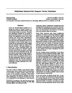
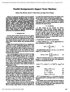
subset. We measure the discrepancy between the full kernel and the uniform-randomsubset Nyström approximation via a few quantities like the maximum difference of ˜ (deeigenvalues and the relative difference of the trace of full kernel K(A, A0 ) and K noted as Max-diff of Eigenvalue and Rel-diff of Trace, respectively in Table 2) on five real datasets, which have manageable sizes of full kernel eigenvalues and eigenvectors. We summarize the results in Table 2. In order to have a better understanding of the differences of their spectral behaviors, we plot four figures for each dataset. Each figure has four subfigures. In subfigure (a), it shows the difference between each pair of eigenvalues. In subfigure (b) and (c), we plot the eigenvalues of the full and the approximate kernels. We split them into two parts and skip the largest eigenvalue because the different scales of eigenvalues. We try to provide more details about them. In subfigure (d), we plot the squared root of eigenvalue of the full kernel 19

times the two norm of the difference of each pair of eigenvectors. That is, we plot √ (k, λk · kek − e˜k k2 ), where λk is the kth eigenvalue of K(A, A0 ) and ek is the corresponding eigenvector. e˜k denotes the kth eigenvector of the Nyström approximation q √ by uniform random subset. Note that λk · kek − e˜k k2 = 2λk (1 − cos θk ), where θk is the angle between ek and e˜k . These angles {θ1 , θ2 , θ3 , . . .} are known as the leading ˜ [7]. canonical angles between K and K We find from these figures that the quality of the approximation will depend on the rate of decay of the eigenvalues of the full kernel matrix. Also, the numerical simulations indicate that the reduced kernel generated by the uniform random selection scheme retains most of the relevant information. These observations might give an explanation why the RSVM can provide a good discriminant and regression function estimation in supervised learning tasks.

20

The Eigen−structure: Full kernel vs. Approx. kernel of Ionosphere dataset 1.5 Full kernel Approx. kernel

40 1

30 20

0.5 10 0

20

40

60

80

0

100

2

4

6 (b)

(a)

3

10

3 Full kernel Approx. kernel

2.5

2.5

2

2

1.5

1.5

1

1

0.5

0.5

0

8

20

40

60 (c)

80

0

100

20

40

60

Figure 1: The spectral analysis of Ionosphere dataset

21

80

100

The Eigen−structure: Full kernel vs. Approx. kernel of Pima dataset 0.5

100

0.4

80

0.3

60

0.2

40

0.1

20

0

20

40

60

80

0

100

Full kernel Approx. kernel

2

4

6 (b)

(a)

1

10


0.8

0.8

0.6

0.6

0.4

0.4

0.2

0.2

0 10

8

20

30 (c)

40

0

50

20

40

60 (d)

Figure 2: The spectral analysis of Pima dataset

22

80

100

The Eigen−structure: Full kernel vs. Approx. kernel of Image dataset 350 Full kernel Approx. kernel

300

1.5

250 200

1

150 100

0.5

50 0

50

100

0

150

5

10

(a)

15

(b)

7


6

2.5

5

2

4 1.5 3 1

2

0.5

1 0

20

40

60

80

100

0

120

(c)

0

50

100 (d)

Figure 3: The spectral analysis of Image dataset

23

150

The Eigen−structure: Full kernel vs. Approx. kernel 15

0.05

Full kernel Approx. kernel

0.04 10 0.03 0.02 5 0.01 0

0

50

100

0

150

5

(a)

10

15

100

150

(b)

0.2 Full kernel Approx. kernel

0.25

0.15 0.2 0.1

0.15 0.1

0.05 0.05 0

50

100

0

150

50

(c)

Figure 4: The spectral analysis of CompActiv (1000) dataset

24

The Eigen−structure: Full Kernel vs Approx. Kernel of Kin−fh−1000 0.01

2.5 Full kernel Approx. Kernel

0.008 0.006 2 0.004 0.002 0

0

50

100

1.5

150

5

10

(a)

15

(b)

0.2 1.5

Full kernel Approx. Kernel 0.15

1 0.1 0.5 0.05

0

20

40

60 (c)

80

0

100

0

50

100 (d)

Figure 5: The spectral analysis of Kin-fh (1000) dataset

25

150

5

Minimaxity and maximinity

In this section we will show that the uniform sampling design in Corollary 1 possesses some other robustness properties, namely, the minimaxity and the maximinity. The ideas are taken from robust designs [41, 42, 43, 22, 1, 2] and customized into the context of the RSVM (4). Recall the full and reduced models: full model : reduced model :

f (x) = f (x) =

m X i=1 m ˜ X

vi K(Ai , x) − γ,

(17)

v˜i K(A˜i , x) − γ.

(18)

i=1

Using kernel K corresponds to mapping the data into a feature Hilbert space with a map: Φ : X → U .3 In the feature space U, the normal vector of the SVM separating hyperplane, w0 u−γ = 0, can be expanded in terms of support vectors. The full model has the following full expansion for the normal vector full pre-image expansion : w =

m X

vi Φ(Ai ),

(19)

i=1

while the reduced model has the reduced expansion reduced pre-image expansion : w =

m ˜ X

v˜i Φ(A˜i ).

(20)

i=1

Expansions given by (19) and (20) are called pre-image expansions [36]. We now try to measure the error induced by the reduced-set approximation. For a given vector v ∈ Rm , we consider the minimization problem minm˜ k

v˜∈R

m X i=1

vi K(Ai , x) −

m ˜ X i=1

3

v˜i K(A˜i , x)k2H(dξT ) .

(21)

Here we assume the kernel spectral is done with respect to the measure ξT , i.e., K(x, z) = R 2 R φi (x)dξT = 1 and φi (x)φj (x)dξT = 0 for i 6= j. The corresponding Hilbert i λi φi (x)φi (z) with

P

space is denoted by H(dξT ).

26

By reproducing property, k

m X

vi K(Ai , x) −

i=1

m ˜ X i=1

˜ A˜0 )˜ v˜i K(A˜i , x)k2H(dξT ) = v 0 K(A, A0 )v − 2v 0 K(A, A˜0 )˜ v + v˜0 K(A, v.

˜ A˜0 )−1 K(A, ˜ A0 )v ∈ Rm˜ solves problem (21). Hence, the Then the vector v˜∗ = K(A, errors induced by the reduced-set approximation (18) and (20) are given respectively by minm˜ k

v˜∈R

m X

vi K(Ai , x) −

i=1

m ˜ X i=1

˜ v˜i K(A˜i , x)k2H(dξT ) = v 0 (K − K)v,

˜ is defined as in (15), and similarly where K = K(A, A0 ) and K minm˜ k

v˜∈R

m X

vi Φ(Ai ) −

i=1

m ˜ X

˜ v˜i Φ(A˜i )k2U = v 0 (K − K)v.

i=1

They lead to the same quantity. Below we define some more notations. All the ξ’s are assumed in the class P given by (10). The full data A is assumed fixed and the reduced set size m ˜ is also assumed fixed. • F(A) := linear span{K(Ai , ·)}m i=1 , which is the full model given training inputs ˜ ˜ := linear span{K(A˜i , ·)}m A. R(A) i=1 , which is a reduced model by the subset

A˜ ⊂ A. We will suppress the set notation and simply use F and R, if no confusion. ˜ ξ := R m˜ K(A, A˜0 )K(A, ˜ A˜0 )−1 K(A, ˜ A0 )dξ(A), ˜ where dξ(A) ˜ = dξ(A˜1 ) · · · dξ(A˜m˜ ). • K X ˜ ξ is an m × m matrix representing the average effect of low-rank approximaK ˜ ξ , it also means tion by ξ-drawn subset of size m. ˜ Note that when we use K T a low-rank approximation by ξT -drawn subset of size m, ˜ but rather not means the full kernel. o

n

˜ ξ )v ≤ η 2 . It specifies a region in F. • Fη− := f (x) = v 0 K(A, x) ∈ F : v 0 (K − K T After removing the average effect explained by ξ-drawn reduced model, we put 27

a bound on what is left unexplained. Later, when we compare the full model and a ξ-drawn reduced model via a certain bias measure, this bound is used to prevent the bias measure from escaping to infinity. • Fη+ :=

n

o

˜ ξ )v ≥ η 2 . It specifies a region in F. f (x) = v 0 K(A, x) : v 0 (K − K T

Again, after removing the average effect explained by reduced model, what is left unexplained has at least H(dξT )-norm of size η. Later, in a lack of fit test (i.e., checking if the ξ-drawn reduced model provides an adequate approximation for functions in Fη+ ) also via a bias measure, the η-distance bounds the bias measure away from zero. In other words, the η-distance guarantees a minimum (> 0) distinguishability between the ξ-drawn reduced model and Fη+ . ˜ := kf (x)−PR f k2 • For f (x) = v 0 K(A, x) ∈ F, define B(f, A) H(dξT ) , where PR f (x) is the projection of f onto R and is given by ˜ A˜0 )−1 K(A, ˜ x). PR f (x) = v 0 K(A, A˜0 )K(A, It is derived by solving a minimization problem similar to (21). This quantity ˜ reflects the bias measure induced by approximating f (x) = v 0 K(A, x) B(f, A) ˜ using the reduced model by subset A. • B(f, ξ) :=

R ˜ Xm

˜ ˜ B(f, A)dξ( A). It is straightforward to show that B(f, ξ) =

˜ ξ )v. The quantity B(f, ξ) reflects an average bias measure induced v 0 (K − K by approximating f (x) = v 0 K(A, x) using the ξ-drawn subset. There are other means of defining alternative classes Fη− and Fη+ and bias measure B(f, ξ), see, for instance, [41, 42, 43, 22, 1, 2]. The minimaxity and maximinity discussed below depend on the particular way of specifying alternative classes and also on the definition of bias measure.

28

Theorem 2 (Minimaxity) The minimax sampling design which minimizes the maximum bias B(f, ξ) for f ∈ Fη− is achieved by ξ = ξT , i.e., sup B(f, ξT ) = inf sup B(f, ξ).

f ∈Fη−

ξ∈P

(22)

f ∈Fη−

Equivalently, the uniform design with respect to ξT is the minimax sampling design. Theorem 3 (Maximinity) For f ∈ Fη+ , the maximin sampling design for B(f, ξ) is achieved by ξ = ξT , i.e., inf B(f, ξT ) = sup inf+ B(f, ξ).

f ∈Fη+

ξ∈P f ∈Fη

(23)

Both the minimaxity and maximinity are some qualities that are robust against the worst case scenarios. Theorem 2 says that the worst expected L2 error, intro˜ ξ v, is minimized by the Nyström approximation duced by the approximation Kv ≈ K ˜ξv using uniform random subset. In judging if a reduced set approximation Kv ≈ K is adequate or not, Theorem 3 says that, for a least distinguishable f ∈ Fη+ , the Nyström approximation by uniform random subset has the best testing power for a lack of fit (i.e., the best ability to detect an inadequacy for a least distinguishable f ). Theorems 2 and 3 tell us that the uniform design (a space filling design) is robust against the worst case. All the statistical properties discussed in this article, including the optimal bases sampling design, the minimaxity and maximinity, are all prior to training phenomena. Though the worst case scenarios or the prior to training phenomena might not sound practical in real experiments, the spectral analysis for real datasets in Section 4 further provides some practical view for the method. Experimental results show that the uniform random subset often provides a reasonably well approximation to the full kernel in ordinary cases.

29

6

Applicability to other kernel-based algorithms

For many other kernel-based algorithms, one has to face the same problems (P1) and (P2) stated earlier. Several authors have suggested the use of low-rank approximations to the full kernel matrix for very large problems [20, 35, 44]. These low-rank approximations all have used a thin rectangular matrix Kmm˜ consisting of a subset of m(¿ ˜ m) columns drawn from the full kernel matrix K. Lee and Mangasarian [20], Williams and Seeger [44] suggest to pick the subset randomly and uniformly over all columns. Smola and Schölkopf [35] consider finding an optimal subset. Since finding an optimal subset is a combinatorial problem involving C(m, m) ˜ possibilities and an exhaustive search is too expensive to carry out, they use a probabilistic speedup algorithm. The trick they use is: First draw a random subset of a fixed size and then pick the best basis (column) from this set. The search goes on till the stopping criterion is reached. For either Lee and Mangasarian’s, or Williams and Seeger’s random subset, or Smola and Schölkopf’s a priori random subset at each iteration in search for an optimal basis within, our theorems and optimality properties are valid referring to the random mechanism of the subset selection. For problems solved in the primal space, e.g., the proximal SVM [14], the leastsquare SVM [38, 39], the kernel Fisher discriminant [30, 29], the random subset method works by replacing the full kernel with the reduced kernel K(A, A˜0 ) and also by cutting down the corresponding number of parameters. For problems solved in the ˜ = K(A, A˜0 )K(A, ˜ A˜0 )−1 K(A, ˜ A0 ) dual space, we form the approximate kernel matrix K to replace the full matrix K. For instance, a reduced set approach for the Lagrangian SVM [28] has been implemented in [23]. To obtain the primal solution v˜, we should ˜ where v is the dual solution. solve K(A, A˜0 )˜ v = Kv, Though we have discussed the statistical properties of the uniform random subset approach mainly on the context of the reduced SVM, the use of a uniform random 30

subset is not limited to the RSVM. The uniform random subset approach can act as a supplemental-algorithm on top of a basic optimization algorithm, wherein the actual optimization takes place on the subset-approximated data. The statistical properties discussed above are still valid.

7

Conclusion

We study the RSVM from a robust design point of view and measure the discrepancy between the full kernel and the uniform-random-subset generated Nyström approximation in order to provide a better understanding of the reduced kernel technique. Our main results center on two major themes. One is on the robustness of the random subset mixture model and the other is on the spectral analysis of the reduced kernel. We show that uniformly and randomly selecting the reduced set of RSVM is the optimal sampling strategy for recruiting kernel bases in the sense of minimizing a model variation measure. We further provide two optimal properties for the RSVM, namely, the minimaxity and maximinity. As for a practical view of the RSVM in action, we have provided some spectral analysis. We compare the eigen-structures of the full kernels and the approximation kernels on five real datasets. The approximation kernels are generated by uniform random subsets. The discrepancies such as the differences between each pair of eigenvalues and eigenvectors, the relative difference of the trace are very small. These results indicate that the uniform random subset kernels can retain most of the relevant information for the learning tasks in the full kernel. We have tested the RSVM on nine datasets and compared the results to the conventional nonlinear SVM solved by the LIBSVM. Although in many cases the RSVM has a slightly bigger training error, it does not scarify any predicting accuracy on all test datasets. Furthermore, the reduced set size is smaller than the number of support vectors in conventional SVM results. Thus, the RSVM uses a simpler model 31

and is more economic in predicting new unlabeled data. This is an advantage in the testing phase of learning tasks. The usage of uniform random subset is not limited to the RSVM. The statistical properties discussed remain valid for other kernel-based algorithms combined with a uniform random subset approximation.

8

Appendix

Lemma 1 For a given nonnegative function t(z), let Pt denote the collection of probability density functions p(z) ∈ P, where P is as defined in (10), such that R

X (t(z)/p(z))dξT (z)

< ∞. (Here 0/0 is defined to be zero.) Then the solution to the

following optimization problem Z

arg min p∈Pt

q

X

(t(z)/p(z))dξT (z)

is given by p(z) = c−1 t(z), where c = Proof: Since

R

X (t(z)/p(z))dξT (z)

R q X

< ∞ and

t(z) dξT (z).

R X

p(z)dξT (z) = 1, by Hölder inequality,

we have Z X

Z

(t(z)/p(z)) dξT (z) =

X

µZ q

Z

(t(z)/p(z)) dξT (z) ·

X

p(z)dξT (z) ≥

X

¶2

t(z)dξT (z)

.

Equality holds if and only if, there exists some nonzero constant β such that t(z)/p(z) = βp(z) a.e. with respect to ξT . q

Since p(z) is a pdf, then equality holds if and only if p(z) = c−1 t(z).

2

˜ ξ 1/c2 ≤ 1. Assume In the rest of proofs, we let c20 = 10 K(A, A0 )1 and ρ0 = 10 K 0 T ˜ ξ is nonnegative definite and 0 ≤ ρ0 < 1. that m ˜ ¿ m, so that K − K T Lemma 2 supf ∈Fη− B(f, ξT ) = η 2 . 32

Proof: For f ∈ Fη− , we have B(f, ξT ) ≤ η 2 . The proof can be completed by finding an f0 ∈ Fη− such that the above equality holds. Let f0 (x) = v00 K(A, x) with v0 = √ ˜ ξ )v0 = η 2 . Here K ˜ξ = η1/(c0 1 − ρ0 ). It is easily verified that v00 (K(A, A0 ) − K T T R

˜ A˜0 )−1 K(A, ˜ A0 )dξT (A). ˜ K(A, A˜0 )K(A,

2

Lemma 3 inf f ∈Fη+ B(f, ξT ) = η 2 . Proof: Similarly, for any f ∈ Fη+ , we have B(f, ξT ) ≥ η 2 . Again by taking f0 (x) = √ ˜ ξ )v0 = η 2 . v00 K(A, x) with v0 = η1/(c0 1 − ρ0 ), we have v00 (K(A, A) − K 2 T Proof for Theorems 2 and 3: We will show that (1) inf ξ∈P supf ∈Fη− B(f, ξ) = supf ∈Fη− B(f, ξT ) and (2) supξ∈P inf f ∈Fη+ B(f, ξ) = inf f ∈Fη+ B(f, ξT ). (1) From Lemma 2 we have supf ∈Fη− B(f, ξT ) = η 2 . Part (1) can be shown by finding an f0 ∈ Fη− such that B(f0 , ξ) ≥ η 2 for all ξ, i.e. finding an f0 (x) = v00 K(A, x) such that ˜ ξ )v0 ≤ η 2 , v00 (K − K T ˜ ξ )v0 ≥ η 2 , ∀ξ. v00 (K − K For ξ 6= ξT , let ν = ξT − ξ, a signed measure. By Hahn decomposition theorem there exists a measurable set E such that ν is positive on E and negative on E c . Let ∗ ∗ v0∗ = (v01 , . . . , v0m )0 be given by

∗ v0i =

q

   1,

if Ai ∈ E,

  0,

if Ai ∈ E c .

˜ ξ )v0∗ . Then B(f0 , ξT ) = η 2 . Since ξ = ξT − ν and ν is Let v0 = ηv0∗ / v0∗ (K − K T 0

˜ ˜ξ − K ˜ ξ )v0 = v 0 K positive on E, we have v00 (K 0 ν v0 ≥ 0. Thus, T ˜ ξ )v0 = v00 (K − K ˜ξ + K ˜ ν )v0 ≥ B(f0 , ξT ) = η 2 . B(f0 , ξ) = v00 (K − K T 33

(2) From Lemma 3 we have inf f ∈Fη+ B(v, ξT ) = η 2 . Part (2) can be shown by finding an f0 ∈ Fη+ such that B(f0 , ξ) ≤ η 2 for all ξ, i.e. finding an f0 (x) = v00 K(A, x) such that ˜ ξ )v0 ≥ η 2 , v00 (K − K T ˜ ξ )v0 ≤ η 2 , ∀ξ. v00 (K − K ∗ ∗ Let ν, E and E c be as defined above. Let v0∗ = (v01 , . . . , v0m )0 be given by ∗ = v0i

q

   0,

if Ai ∈ E,

  1,

if Ai ∈ E c .

˜ ξ )v0∗ . Then B(f0 , ξT ) = η 2 . Since ξ = ξT − ν and ν is Let v0 = ηv0∗ / v0∗ (K − K T 0

˜ξ − K ˜ ξ )v0 = v 0 K ˜ negative on E c , we have v00 (K 0 ν v0 ≤ 0. Thus, T ˜ ξ )v0 = v00 (K − K ˜ξ + K ˜ ν )v0 ≤ B(f0 , ξT ) = η 2 . B(f0 , ξ) = v00 (K − K T The proof is completed.

2

Kernel boundary correction. The issue of making boundary kernels and doing boundary correction in nonparametric estimation and prediction is a pretty subtle problem and there is vast statistical literature. See, e.g., Gasser, M¨ uller and Mammitzsch [15] and references therein. Here we only provide some most basic ideas of boundary kernels and boundary correction. Let B be the set of the so called boundary points, which consist of points on and near the boundary. For simplicity consider translation-type kernels that are probability density functions. Boundary kernels are a collection of continuous varying kernels (with respect to z) {K(·, z)}z∈B satisfying R

K(x0 , z)dx = 1. For instance, one simple way to make Gaussian boundary kernels

is to fold the part of kernel outside X by reflection and add it to the interior part. Another way is simply to rescale kernels near the boundary and make them integrate to one. To correct the boundary effects, one conceptually simple way is to replace the ordinary kernels with boundary kernels for points z near the boundary. 34

Acknowledgment The authors wish to acknowledge the helpful comments and suggestions by three anonymous referees, which have enhanced the paper. The authors also thank Olvi Mangasarian for his suggestions and Hwang, Chii-Ruey for discussion and comments on the sampling design and spectral analysis and for reading the manuscript.

References [1] S. Biedermann and H. Dette. Minimax optimal designs for nonparametric regression - a further optimality property of the uniform distribution. Advances in Model-oriented Design and Analysis, pages 13–20, 2001. [2] S. Biedermann and H. Dette. Optimal designs for testing the functional form of a regression via nonparametric estimation techniques. Statist. Probab. Letters, 52:215–224, 2001. [3] C. L. Blake and C. J. Merz. UCI repository of machine learning databases, 1998. http://www.ics.uci.edu/∼mlearn/MLRepository.html. [4] C. J. C. Burges. A tutorial on support vector machines for pattern recognition. Data Mining and Knowledge Discovery, 2(2):121–167, 1998. [5] C.-C. Chang and Y.-J. Lee. Generating the reduced set by systematic sampling. In Zheng Rong Yang, Richard Everson, and Hujun Yin, editors, Proceedings of the Fifth International Conference on Intelligent Data Engineering and Automated Learning(LNCS 3177), pages 714–719, Exeter, UK, 2004. Springer–Verlag. [6] C.-C. Chang and C.-J. Lin. LIBSVM: a library for support vector machines, 2001. Software available at http://www.csie.ntu.edu.tw/~cjlin/libsvm.

35

[7] F. Chatelin. Eigenvalues of Matrices. John Wiley & Sons, Chichester, 1993. [8] N. Cristianini and J. Shawe-Taylor. An Introduction to Support Vector Machines. Cambridge University Press, Cambridge, 2000. [9] Delve. Comp-activ dataset, data for evaluating learning in valid experiments. http://www.cs.toronto.edu/∼delve/data/comp-activ/desc.html. [10] Delve. Kin-family of datasets, data for evaluating learning in valid experiments. http://www.cs.toronto.edu/∼delve/data/kin/desc.html. [11] H. Drucker, C. J. C. Burges, L. Kaufman, A. Smola, and V. Vapnik. Support vector regression machines. In M. C. Mozer, M. I. Jordan, and T. Petsche, editors, Advances in Neural Information Processing Systems -9-, pages 155–161, Cambridge, MA, 1997. MIT Press. [12] K. T. Fang, D. K. J. Lin, P. Winker, and Y. Zhang. Uniform design: theory and application. Technometrics, 42:237–248, 2000. [13] K. T. Fang, Y. Wang, and P. M. Bentler. Some applications of number-theoretic methods in statistics. Statistical Science, 9:416–428, 1994. [14] G. Fung and O. L. Mangasarian. sifiers.

Proximal support vector machine clas-

In F. Provost and R. Srikant, editors, Proceedings KDD-2001:

Knowledge Discovery and Data Mining, August 26-29, 2001, San Francisco, CA, pages 77–86, New York, 2001. Asscociation for Computing Machinery. ftp://ftp.cs.wisc.edu/pub/dmi/tech-reports/01-02.ps. [15] T. Gasser, H-G. M¨ uller, and V. Mammitzsch. Kernels for nonparametric curve estimation. J. Roy. Statist. Soc. B, 47:238–252, 1985.

36

[16] T. Hastie, R. Tibshirani, and J. Friedman. The Elements of Statistical Learning. Springer-Verlag, New York, 2001. [17] L.-R. Jen and Y.-J. Lee. Clustering model selection for reduced support vector machines. In Zheng Rong Yang, Richard Everson, and Hujun Yin, editors, Proceedings of the Fifth International Conference on Intelligent Data Engineering and Automated Learning(LNCS 3177), pages 720–725, Exeter, UK, 2004. Springer–Verlag. [18] Y.-J. Lee, W.-F. Hsieh, and C.-M. Huang. ²-SSVR: A smooth vector machine for ²-insensitive regression. IEEE Transactions on Knowledge and Data Engineering, 17:678–685, 2005. [19] Y.-J. Lee, H.-Y. Lo, and S.-Y. Huang. Incremental reduced support vector machine. In International Conference on Informatics Cybernetics and System (ICICS 2003), Kaohsiung, Taiwan, 2003. [20] Y.-J. Lee and O. L. Mangasarian. RSVM: Reduced support vector machines. Technical Report 00-07, Data Mining Institute, Computer Sciences Department, University of Wisconsin, Madison, Wisconsin, July 2000. Proceedings of the First SIAM International Conference on Data Mining, Chicago, April 5-7, 2001, CD-ROM Proceedings. ftp://ftp.cs.wisc.edu/pub/dmi/tech-reports/00-07.ps. [21] Y.-J. Lee and O. L. Mangasarian. machine.

SSVM: A smooth support vector

Computational Optimization and Applications, 20:5–22, 2001.

Data Mining Institute, University of Wisconsin, Technical Report 99-03. ftp://ftp.cs.wisc.edu/pub/dmi/tech-reports/99-03.ps. [22] K. C. Li. Robust regression designs when the design space consists of finitely many points. Ann. Statist., 12:269–282, 1984. 37

[23] K.-M. Lin and C.-J. Lin. A study on reduced support vector machines. IEEE Transactions on Neural Networks, 14:1449–1459, 2003. [24] J. S. Liu. Monte Carlo Strategies in Scientific Computing. Springer–Verlag, New York, 2001. [25] O. L. Mangasarian.

Generalized support vector machines.

In A. Smola,

P. Bartlett, B. Schölkopf, and D. Schuurmans, editors, Advances in Large Margin Classifiers, pages 135–146, Cambridge, MA, 2000. MIT Press. ftp://ftp.cs.wisc.edu/math-prog/tech-reports/98-14.ps. [26] O. L. Mangasarian and D. R. Musicant. Large scale kernel regression via linear programming. Technical Report 99-02, Data Mining Institute, Computer Sciences Department, University of Wisconsin, Madison, Wisconsin, August 1999. ftp://ftp.cs.wisc.edu/pub/dmi/tech-reports/99-02.ps. [27] O. L. Mangasarian and D. R. Musicant. Robust linear and support vector regression. IEEE Transactions on Pattern Analysis and Machine Intelligence, 22(9):950–955, 2000. ftp://ftp.cs.wisc.edu/pub/dmi/tech-reports/99-09.ps. [28] O. L. Mangasarian and D. R. Musicant. tor machines.

Lagrangian support vec-

Journal of Machine Learning Research, 1:161–177, 2001.

ftp://ftp.cs.wisc.edu/pub/dmi/tech-reports/00-06.ps. [29] S. Mika. Kernel Fisher Discriminants. PhD thesis, Electrical Engineering and Computer Science, Technische Universität Berlin, 2002. [30] S. Mika, G. Rätsch, J. Weston, B. Schölkopf, and K.-R. M¨ uller. Fisher discriminant analysis with kernels. Neural Networks for Signal Processing, IX:41–48, 1999.

38

[31] T. M. Mitchell. Machine Learning. McGraw-Hill, Boston, 1997. [32] E. Parzen. On estimation of a probability density function and mode. Ann. Math. Statist., 35:1065–1076, 1962. [33] C. E. Rasmussen and Z. Ghahramani.

Occam’s razor.

In Todd K. Leen,

Thomas G. Dietterich, and Volker Tresp, editors, Advances in Neural Information Processing Systems 13, pages 294–300, Cambridge, MA, 2001. MIT Press. [34] M. Rosenblatt. Remarks on some nonparametric estimates of a density function. Ann. Math. Statist., 27:832–835, 1956. [35] A. Smola and B. Schölkopf. Sparse greedy matrix approximation for machine learning. In Proc. 17th International Conf. on Machine Learning, pages 911–918. Morgan Kaufmann, San Francisco, CA, 2000. [36] A. Smola and B. Schölkopf. Learning with Kernels. MIT Press, Cambridge, MA, 2002. [37] A. Smola and B. Schölkopf. A tutorial on support vector regression. Statistics and Computing, 14:199–222, 2004. [38] J. A. K. Suykens and J. Vandewalle. Least squares support vector machine classifiers. Neural Processing Letters, 9(3):293–300, 1999. [39] J. A. K. Suykens and J. Vandewalle. Multiclass least squares support vector machines. In Proceedings of IJCNN’99, pages CD–ROM, Washington, DC, 1999. [40] V. N. Vapnik. The Nature of Statistical Learning Theory. Springer, New York, 1995. [41] D. P. Wiens. Designs for approximately linear regression: Two optimality properties of uniform designs. Statist. & Probab. Letters, 12:217–221, 1991. 39

[42] D. P. Wiens. Minimax designs for approximately linear regression. J. Statist. Plann. Inference, 31:353–371, 1992. [43] D. P. Wiens. Minimax robust designs and weights for approximately specified regression models with heteroscedastic errors. J. Amer. Statist. Assoc., 93:1440– 1450, 1998. [44] C. K. I. Williams and M. Seeger. Using the Nyström method to speed up kernel machines. In Todd K. Leen, Thomas G. Dietterich, and Volker Tresp, editors, Advances in Neural Information Processing Systems 13, pages 682–688, Cambridge, MA, 2001. MIT Press. [45] I. H. Witten and E. Frank. Data Mining: Practical Machine Learning Tools and Techniques with Java Implementations. Morgan Kaufmann, San Francisco, CA, 1999.

40