A MISR cloud-type classifier using reduced Support Vector Machines ´ Dominic Mazzoni1 , Akos Horv´ ath1 , Michael J. Garay2 , Benyang Tang1 , and Roger Davies1 1. Jet Propulsion Laboratory, California Institute of Technology, Pasadena, CA 91109, USA
[email protected] 2. University of California, Los Angeles Los Angeles, CA 90095, USA
[email protected] Abstract. We are developing a pixel-level cloud-type classifier for the Multi-angle Imaging SpectroRadiometer (MISR), an instrument used to study clouds and aerosols from NASA’s Terra satellite. To augment MISR’s existing high-level products (including cloud masks, cloud heights, and aerosol optical depth retrievals), our cloudtype classifier labels each 1.1-km pixel as clear, or as belonging to one of several types of cloud. In the past, similar classifiers have been developed for other remote-sensing instruments using various machine learning techniques, such as artificial neural networks. However, support vector machines (SVMs) are not typically used, in part because the computational cost of evaluating new examples with an SVM can be much higher. Our novel approach to achieving high classification accuracy within the computational requirements of the operational MISR processing system involves training a very large multi-class SVM using thousands of training points and then applying cutting-edge reduced-set techniques to yield a computationally manageable number of support vectors. The resulting product will help provide new insights for those constructing cloud climatologies, modeling radiative transfer through clouds, and studying the effects of clouds on climate, in addition to demonstrating the effectiveness of using SVMs in a production science setting.
data analysis it is useful to separate stratiform (layered) clouds from cumuliform (puffy) clouds, at the very minimum. This is because the radiative and hydrological impacts of these two cloud types are very different. Stratiform clouds are thin and relatively dry clouds that cover large areas. They have a profound effect on the radiative properties of the earthatmosphere system due to their ability to reflect large amounts of solar radiation back to space. However, stratiform clouds contain only a very small portion of the total atmospheric liquid water. Cumuliform clouds behave in the opposite manner. These clouds cover small areas and have only a small radiative impact, but contain most of the atmospheric liquid water. Additionally, these two cloud types are indicative of the direction of atmospheric heat transport: stratiform clouds tend to transport heat horizontally, while cumuliform clouds represent heat transport primarily in the vertical.
A second motivation for classifying satellite observations of clouds into different cloud types is that this allows satellite observations to be related to surfacebased observations. Surface weather observers are trained to group clouds into 10 standard types and extensive global compliations exist of these observations. Comparison between satellite and surface observations is facilitated by grouping satellite measurements into similar categories. The International Satellite Cloud Climatology Project (ISCCP), for example, attempts to do this by associating exactly one cloud type with particular ranges of cloud-top height and cloud optical thickness [1]. However, comparisons of ISCCP and surface climatologies (e.g., Hahn et 1 Scientific Motivation al. [2]) have found that this simple approach does Because different cloud types are formed by different not quite work properly and ISCPP can only reliably mechanisms, cloud type is often indicative of underly- distinguish a limited set of combined cloud classes. ing atmospheric processes. In that regard, in satellite Clearly, it would be desirable to do better.
An increasingly important motivation for cloud classification in satellite imagery is climate monitoring. Global changes in the amounts of different cloud types is a potential signal of climate change. Within the operational forecast community as well there is interest in methods of automatic satellite cloud classification. Although weather forecasters typically rely on imagery from geostationary satellites, such as the Geostationary Operational Environmental Satellites (GOES), techniques for automatic cloud classification developed for other satellite instruments, such as the Multi-angle Imaging SpectroRadiometer (MISR) onboard NASA’s Terra satellite, could potentially lead to new insights that could be incorporated into an automatic cloud classifier for GOES imagery.
tures. Saitwal et al. [10] extended Tian et al.’s work to nighttime classification. Baum et al. [11] used fuzzy logic to detect multilayer systems in AVHRR scenes based on examples getting classified into more than one of eight trained cloud types. Azimi-Sadjadi and Zekavat [12] used a hierarchical arrangement of support vector machines to classify six different cloud types in infrared GOES-8 imagery, while Lee et al. [13] investigated using a multi-class support vector machine to distinguish between ice and water clouds in MODIS images. Li et al. [14] used the maximum likelihood technique to improve on the basic cloud classification provided in the MODIS standard product.
3 2
Background
Related Work
Perhaps the most visible example of automatic cloudtype classification using machine learning is Bankert’s real-time classifier for GOES images available on the web [3]. While the classification algorithm it uses is simple (1-nearest-neighbor), the features were selected carefully using a backward sequential selection (BSS) algorithm, and the system boasts an impressively large collection of training data (10 cloud types classified in over 5,000 GOES scenes). More details about the approach are described in a Tag, Bankert et al. paper on Advanced Very High Resolution Radiometer (AVHRR) cloud-type classification [4]. Overall their approach leads to fast and accurate classification. However, some shortcomings are apparent, including limited detection of thin cirrus clouds and small cumulus clouds, as well as multilayer systems of cirrus over low clouds being misclassified as mid-level clouds. The latter problem, in particular, occurs when low and high cloud infrared temperatures are averaged to obtain the associated cloud height, a problem that would be alleviated if cloud heights could be determined by another method. Dozens of other papers exist on automatic satellite cloud-type classification using learning algorithms. Some pioneering work was done by Welch et al. [5], comparing the use of discriminant analysis and two types of neural networks to classify pixels in AVHRR images as one of a number of classes, including five cloud types. Bankert et al. [6] [7] [8] compared neural networks to decision trees and a 1-nearest-neighbor classifier in GOES data. Tian et al. [9] used probabalistic neural networks to classify 10 cloud types in GOES images using both spatial and temporal fea-
We used Support Vector Machines (SVMs) to construct a cloud-type classifier for image data from the Multi-angle Imaging SpectroRadiometer (MISR) satellite instrument. This section provides a brief overview of SVMs and the characteristics of the MISR instrument. 3.1
Support Vector Machines
SVMs [15] are a popular technique for supervised classification. Training a binary SVM is a quadratic optimization procedure that finds an optimal hyperplane separating positive and negative example vectors, balancing accuracy with generalization performance by maximizing the margin. The margin is simply the distance from the hyperplane to the nearest positive and negative labeled feature vectors. However, since most problems are not linearly separable, SVMs typically use a kernel function that implicitly projects two example vectors in input space (Xi , Xj ) into (possibly infinite) feature space vectors (Φ(Xi ), Φ(Xj )) and returns their dot product in that feature space. Popular kernels (with model selection parameters a, p, σ) include: linear: K(u, v) = u · v, polynomial: K(u, v) = (u · v + a)p , RBF: K(u, v) = exp(− 2σ1 2 ||u − v||2 ) It is also common to use normalized kernels, which makes it more practical to work with high-degree polynomials: 1
1
Knorm (u, v) := K(u, v)K(u, u)− 2 K(v, v)− 2
km × 1.1 km per pixel (plus limited coverage at 275 m × 275 m). The images are projected to a common grid and coregistered during automatic ground processing, resulting in nine views of each scene with a swath width of about 350 km. There are at least three ways that MISR’s multiple angles yield cloud information not available via conventional satellite means. First, thin clouds and aerosols are more opaque at oblique angles because the photon path length is longer, making these atmospheric constituents more apparent against the background surface. Second, objects in MISR imagery can be identified by their angular signature. Because aerosols and clouds scatter radiation differently into different directions at different wavelengths, this knowledge can be exploited to help characterize clouds and aerosols. Third, because the cameras are registered to the surface ellipsoid, objects above the surface appear displaced due to the parallax effect (see Figure 1). Operationally, an automatic pattern-matching algorithm is used in the instrument software to determine the disparity of each pixel and infer the height using triangulation. This is complicated by the fact that there is a seven minute delay between the imaging times of the first and last cameras to view each scene and approximately a one minute delay between images taken by each camera, during which time clouds may have moved. However, the cloud-top height (± 500 m at a spatial resolution of 1.1 km) and the height-resolved mesoscale wind (± 4 m/s at a spatial resolution of 70.4 km) can be retrieved operationally by various stereoscopic combinations of views [19] [20]. The stereoscopicallyderived height provides an independent check against the cloud-top height measurements made by other instruments using measurements of emitted radiation and assumptions about the thermal structure of the atmosphere. While several methods have been developed to obtain scientifically useful measurements from multiangle satellite data, the full parameter space of infor3.2 MISR mation remains largely unexplored. We have found The Multi-angle Imaging Spectroradiometer (MISR) that machine learning techniques allow us to explore is one of five instruments aboard NASA’s Terra satel- this parameter space much more quickly. lite, which follows LandSat 7 in polar orbit around the Earth at an altitude of 705 km with an equatorial crossing time of 10:30 am (local time) for the 4 Previous Work descending portion of the orbit. MISR has nine pushbroom cameras pointed in different directions along This work builds on our previous successes developthe orbital path, ranging from 70◦ forward to 70◦ aft- ing pixel classifiers for MISR [21]. We created a biward. Each camera views four spectral bands (blue, nary cloud mask (distinguishing cloudy pixels from green, red, and near-infrared) with a resolution of 1.1 clear pixels) using a total of 156 features as input.
The hyperplane resulting from SVM training is defined implicitly by a vector of weights αi on the original training examples. Many of these αi will be zero and the associated example vectors can be discarded. The example vectors whose corresponding αi is nonzero – called support vectors – are needed in order to determine the classification of new points. Note that when a linear kernel is used, it is possible to compute the hyperplane normal vector by summing the α-weighted support vectors. For any nonlinear kernel, though, the hyperplane normal vector exists in feature space and may not have a pre-image in input space. As a result, classifying a new example using a SVM can be expensive, requiring one dot-product calculation per support vector. Because more difficult classification problems tend to require more support vectors, SVMs have developed a reputation for being powerful but inefficient. SVM reduced-set methods [16] use various techniques to decrease the number of support vectors, either by eliminating those support vectors that contribute the least (and re-weighting the remaining ones) or by explicitly solving for the pre-image of the hyperplane normal vector. While previous results have shown impressive reductions in the number of support vectors with minimal loss of generalization performance on some problems, many other problems proved to be irreducible, and the reduction algorithms were typically very slow. However, recent breakthroughs (described in greater detail below) have resulted in even more sophisticated reduced-set techniques that overcome many of these limitations. Although there have been methods developed for “true” multi-class SVMs (e.g., [17]), it is usually more practical to perform multi-class classification by training several binary SVMs [12] [18]. Common methods for solving multi-class problems using binary SVMs include one-vs-one, one-vs-all, and directed acyclic graph (DAG).
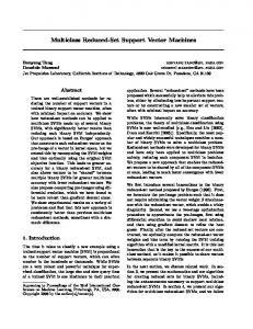
Fig. 1. On the left, MISR’s view of multilayer clouds over the Molucca Sea, with the northeastern tip of the Indonesian island of Sulawesi in the upper-left of the image, taken on December 1, 2004. On the right, MISR’s 70-degree forward view of the same scene. Note both the increased opacity of the cirrus clouds and the vertical displacement of the clouds due to their height above the surface. Path 111, Orbit 26354, Blocks 89-90, courtesy Langley Atmospheric Sciences Data Center.
The features were derived from raw MISR radiances from all four spectral bands and the three most nadirpointing cameras, as well as several neighboring pixels for context. We trained two separate SVMs: one specializing in clouds over water and one over land (the MISR standard product identifies whether each pixel is over water or over land). We used two of MISR’s existing cloud masks to provide training labels for these two SVMs, but only over surfaces where we knew the existing cloud masks tended to be accurate. The resulting SVMs we trained over water and land had 656 and 2456 support vectors, respectively. To validate the performance, we independently labeled 3,500 pixels randomly distributed throughout the globe, finding that the existing cloud masks each had error rates of approximately 12% relative to these expert labels, while our SVM cloud mask had an error rate of approximately 6%. Subsequently, we developed improved reduced-set techniques that successfully reduced both SVMs used in the cloud mask to 20 support vectors each. The accuracy of the land SVM remained unchanged, while the accuracy of the water SVM decreased by only 0.3%. The resulting classifier requires just slightly more than 156 × 20 multiply-add instructions per pixel, which we determined was fast enough to run as part of the standard MISR data processing. We have completed a test of processing the SVM cloud mask at the NASA Langley Atmospheric Sciences Data Center and are working on integrating it and making it available as a standard MISR product later this year.
We also developed two other binary classifiers for MISR using the same approach. Thin cirrus clouds can have potentially large radiative effects on the atmospheric and surface energy budgets and they present an impediment to the operational retrieval of clear sky atmospheric and surface properties. However, thin cirrus clouds are notoriously difficult to detect using standard satellite remote sensing techniques. Our SVM cirrus cloud detector was trained using expert labels with essentially the same inputs as the cloud mask described above. However, instead of using the three most nadir pointing MISR cameras, we used the three most forward cameras in the northern hemisphere and three most aftward cameras in the southern hemisphere. This approach took advantage of the unique capabilities of MISR relative to other instruments by utilizing the increased path length of photons being scattered in the forward direction at these oblique viewing angles. Finally, a SVM smoke detector was developed to distinguish smoke and some related aerosols from cloudy and clear pixels in MISR imagery. Because the detection, as opposed to the precise location, of the smoke was of primary interest, we experimented with using data from five of MISR’s nine cameras as input. This resulted in improved detection of smoky regions due to the increased photon path length for the oblique cameras used, as well as the characteristic angular signature of smoke, which was made more apparent through the use of a larger number of angles. These two classifiers have been validated, but not yet to the
same degree of precision as the cloud mask. We hope to finish the validation effort and make both these classifiers available as MISR data products later in the year, as well.
5
Methodology
Our previous three MISR classifiers were binary (e.g. cloudy vs. clear). As our goal in this new research was to develop a cloud-type classifier, we needed to deal with many new issues associated with a multiclass learning problem, such as how to handle examples that could conceivably belong to more than one class. After choosing the classes to label, we began by creating expert labelings of 30 scenes, each one approximately a quarter of a MISR swath, about 400 × 5, 000 pixels. Our strategy was not to label every pixel, nor to choose individual scattered pixels; instead we used a graphical interface to rapidly “paint” labels over the top of the image wherever we were reasonably confident about the classification, avoiding cloud edges and multilayer systems. Using this technique we labeled over 3 million pixels across the 30 scenes. With practice, we found that MISR is particularly amenable to expert labeling by visual inspection, because we could rapidly flip between the different camera views of one scene and see its unambiguous three-dimensional structure. We originally considered 12 classes, made up of 4 non-cloud classes and 8 cloud types, but later combined some of the classes that were difficult to distinguish, resulting in the choice of the following eight classes: Abbrev. Ocean Land Ice m Sc sm Cu Cb Ci St
Class Clear Ocean Clear Land Ice or Snow Marine Stratus or Stratocumulus Small Cumulus Cumulus Congestus or Cumulonimbus Cirrus Other Stratiform
Examples from every class showed up in at least three distinct scenes. To construct the feature vectors for classification, we started with the feature vector we used successfully for cloud detection, which will now be described in greater detail. One of the principal ideas behind our feature vectors is deceptively simple: in order to
classify a single pixel, we use all the values from a 5 × 5 (or larger) region of pixels surrounding the central pixel as features. One source of inspiration for this idea was the observation that SVMs were able to successfully classify images of handwritten digits from the MNIST database with a feature vector consisting simply of all of the 27 × 27 grayscale values making up the image [22]. Using these feature vectors, we trained a multiclass SVM using the one-vs-all method. Of the 30 labeled scenes available, we arbitrarily chose 24 for training and 6 as holdouts for validation. To choose the SVM hyperparameters (the kernel function and regularization parameter C), we chose 2,000 training examples (250 from each class) and 2,000 test examples. We then exhaustively searched a space of several dozen kernel functions and values of C from 0.1 . . . 3000, training a multi-class SVM with each set of parameters. We chose the kernel and C combination that had roughly the lowest test error. However, all other things being equal, we favored parameters that resulted in fewer support vectors, based on our general observation that the same accuracy with fewer support vectors is more likely to generalize. The best choice turned out to be a normalized polynomial kernel with p = 17 and a = 1, and C = 50. After selecting the hyperparameters, we trained a larger SVM using 8,000 training examples (1,000 from each class) using the one-vs-all method. (We also tried one-vs-one and got similar results, but one-vs-all was preferable for reducing, as will be seen later.) On a holdout set of 8,000 examples, the overall accuracy was 78.6%, with the following confusion matrix: Ocean Land Ice m Sc sm Cu Cb Ci St Ocean 88.2% 0.0% 0.0% 0.6% 10.5% 0.0% 0.7% 0.0% Land 0.0% 99.7% 0.0% 0.0% 0.1% 0.0% 0.2% 0.0% Ice 0.0% 0.0% 58.5% 0.2% 0.8% 21.2% 13.1% 6.2% m Sc 0.5% 0.0% 0.1% 66.7% 10.1% 13.6% 3.7% 5.3% sm Cu 18.1% 2.9% 0.1% 12.5% 61.9% 0.0% 4.5% 0.0% Cb 0.0% 0.0% 4.0% 7.0% 0.1% 87.1% 1.5% 0.3% Ci 1.2% 0.3% 0.2% 5.4% 7.2% 2.9% 82.8% 0.0% St 0.0% 0.0% 0.0% 4.4% 0.0% 9.9% 0.7% 85.0%
From the confusion matrix, we gathered that the most difficult classes to separate were ice, marine stratocumulus and small cumulus. Interestingly, we found that ice was often being misclassified as cumulonimbus, perhaps because they are both highly reflective surfaces. However, it would be easy to distinguish between these two classes with additional height information available from MISR.
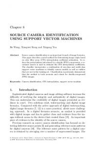
Fig. 2. On the left is the image of the automatically generated stereo height product for the MISR image seen in Figure 1. Darker-colored pixels are higher above the surface, up to a maximum of about 12 km in this particular scene. The noise is mainly due to blunders from the stereo matching algorithm. On the right is the smoothed stereo image used to provide an additional feature for our SVM. Ocean Land Ice m Sc sm Cu Cb Ci St The misclassification of small cumulus as ocean Ocean 87.9% 0.0% 0.0% 0.6% 8.5% 0.0% 3.0% 0.0% (and vice versa) is not unexpected. Small cumulus Land 0.0% 99.9% 0.0% 0.0% 0.1% 0.0% 0.0% 0.0% Ice 0.0% 0.0% 87.2% 1.0% 1.5% 1.7% 2.5% 6.1% cloud fields are often broken, which allows the ocean m Sc 0.4% 0.0% 0.3% 71.0% 9.8% 7.7% 4.1% 6.7% surface to be seen between clouds. This will create sm Cu 14.3% 4.3% 0.0% 12.8% 68.1% 0.1% 0.4% 0.0% Cb 0.0% 0.0% 0.1% 6.0% 0.2% 92.1% 1.4% 0.2% particular difficulties at the edges of cloud fields. The Ci 0.4% 0.4% 0.0% 3.0% 1.7% 2.9% 91.6% 0.0% vertical development of these clouds also introduces St 0.0% 0.0% 0.0% 1.6% 0.0% 9.4% 1.2% 87.8% a parallax effect that can cause the classifier to incorrectly classify pixels as cloudy because clouds are The confusion matrix shows that the most challenging classes all improved their accuracies significantly. seen in one camera and not another.
5.2 5.1
Incorporating stereo height
Initially we were concerned about incorporating height information because MISR’s stereo-derived height product, while extremely accurate overall, tends to be noisy at the pixel level. Therefore, we developed an appropriate smoothing algorithm for this product to allow its use as an additional input for our feature vectors. An image of the stereo height product before and after smoothing can be seen in Figure 2. Adding the smoothed stereo height to our feature vector resulted in significant improvement in the classifier performance as shown in the confusion matrix below. Overall, after incorporating stereo height, the accuracy improved from 78.6% to 85.5%:
Smoothing the results and applying the cloud mask
The resulting multi-class SVM classified each pixel as one of eight different classes. Based on visual inspection of the results, in many regions the classification appeared to be quite good. However, we found that the resulting classification images were quite noisy. As was done in [4] and several other cloud-type classifiers, we attempted to smooth the resulting image and avoid noise. The results of our smoothed classification can be seen in Figure 3. Rather than just using the class of each pixel in the smoothing, we found it was advantageous to use the relative weights of each binary SVM in the smoothing process, taking advantage of the fact that we were using a one-vs-all multi-class SVM. In the one-vs-all paradigm, one binary SVM for each class is designed to determine whether the example is in that class, or in one of the other classes. The output of the binary SVM is a scalar, indicating the distance between that example and the decision hyperplane, with a larger
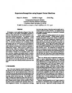
Fig. 3. On the left is the same MISR image seen in Figure 1. On the right, the result of our final, smoothed cloud-type classification algorithm, which has detected regions of cumulonimbus (Cb), cirrus (Ci), some small cumulus clouds (sm Cu), some small marine stratocumulus (m Sc), water and land.
value indicating a farther distance from the hyperplane and the sign indicating whether it falls on the positive or negative side. Class membership is then decided by taking the argmax of all of the binary SVMs. So for every pixel we have a vector of eight binary SVM outputs, one for each of our eight classes. In the simplest case, one of these outputs will be positive and the other seven will be negative, indicating that the pixel in question clearly belongs to one class. However, for ambiguous pixels, or those on the border between regions, several classes may have positive values, in which case the largest one is chosen as the most likely class. In order to smooth the classifier, then, we averaged each vector with the vectors of several neighboring pixels, with a neighbor contributing less depending on the square of its distance from the pixel in question. After this averaging, the argmax of each vector was taken to determine the class. To better understand the consequences of this type of smoothing, consider a single, isolated pixel classified as class 1, when all of its neighbors were classified as class 2. If the isolated pixel was very confidently class 1 (the class 1 binary SVM output was very large, and the other values were very negative), the averaging would not change anything. However, if the isolated pixel was right on the border, perhaps with classes 1 and 2 having almost equal weight, then the averaging would change the pixel’s classification to class 2. We felt that this strategy did the best job of encouraging regions to be more homogeneous while allowing small heterogeneous regions when they were detected with above average confidence. One could
imagine making the degree of smoothing a tunable parameter. Finally, in generating the final cloud-type classification product, we made use of our existing SVM cloud mask and the existing MISR land/water classification to refine our results. The idea is that when training our cloud-type classifier, we were focusing on how best to distinguish between different types of clouds, and less on how to determine whether a pixel was cloudy or clear. Especially after our smoothing, we found that far more pixels were classified as some type of cloud than would normally be considered cloudy pixels. Therefore, as an additional pass, we replaced each pixel which our SVM cloud mask marked as “clear,” with either the clear land or clear water class, as appropriate.
5.3
Reducing the multi-class SVM
Several higher-level products are generated from the raw radiance data and distributed along with MISR data. These include several cloud masks, the stereoderived height products, aerosol optical depths, and top-of-atmosphere albedos. Our goal was to create a classifier that was computationally fast enough that we could integrate it into the data processing system that automatically generates MISR products at the Langley Atmospheric Sciences Data Center. While it was difficult to determine the exact amount of processing time potentially available, very roughly we determined that we could run a single binary SVM that gathered approximately 150 features and used
in the vicinity of 200-300 support vectors. Unfortunately, the multi-class SVM we had trained to do cloud-type classification had 3,340 support vectors (total, including all eight binary SVMs in the onevs-all framework), at least one order of magnitude too many.
to 85.5% accuracy for the unreduced SVM. In the future, we hope to develop methods that “share” support vectors between different binary SVMs within the multi-class classifier for possibly even greater reductions. However, our current techniques have given us SVMs that are at least in the right order of magSome of our previous research includes methods to nitude that we can experiment with running them in classify new examples using SVMs more efficiently the operational MISR software framework. [23] by reordering the support vectors on the fly, skipping most of the support vectors for “easy” examples, and only using the full SVM for the most difficult 6 Conclusions and Future Work (ambiguous) examples. While we have seen speedups as high as 12× with this technique, actual speedups We have investigated the use of SVMs to perform on this particular problem were less, and any efficient cloud-type classification of individual pixels in MISR implementation of this algorithm is enormously more data. Using a combination of radiance and stereo complicated than the normally straightforward SVM height information and a large amount of training evaluation formula, making it a poor candidate for data, we were able to train a classifier that could integrating into a production software system. classify over 85% of the pixels correctly, relative to Instead, we investigated the use of reduced-set human expert labels. Additionally, reduced-set techmethods [16], which attempt to approximate the hy- niques were developed and applied to yield more efperplane normal vector using a small number of vec- ficient SVMs with similiar accuracy, but much faster tors instead of all of the support vectors. While we runtime for use in an operational setting. found the theory to be quite solid, the pre-image We hope that this research helps open the door for algorithm in [16], which maps a feature space vec- future use of SVMs in remote-sensing pixel classificator back to the input space, often got stuck in local tion problems. While neural networks, decision trees, minima, making the reduction process very frustrat- genetic algorithms, and several other techniques have ing. Therefore, we developed our own pre-image al- been popular in such problems for years, support vecgorithm, using Differential Evolution [24] to find a tor machines have many advantages, and now that rough pre-image, then applying gradient descent to it is possible to use them with no associated speed refine it. Another improvement we made is that after penalty, they should be considered more often. the reduced-set vectors have been computed we readOur immediate plans are to further develop our just the weights and bias through a modified SVM reduced-set techniques for multi-class support vector training algorithm. The details of our approach will machines, continue to refine our cloud classifier with be presented in a future paper. more training examples and eventually turn a final We had great success applying our new reduced-set version of the classifier into an operational product. method to binary SVMs, for example reducing our bi- In addition, we intend to explore incorporating texnary cloud mask over land from 2456 support vectors ture features, which are likely to help distinguish beto exactly 20, with essentially no loss in overall accu- tween certain classes of clouds. racy. We are still researching the best way to reduce a multi-class SVM. One straightforward technique that we have used successfully is to reduce each of the in7 Acknowledgements dividual binary SVMs in a one-vs-all classifier, allocating a different number of support vectors to each binary classifier based on its difficulty. Specifically, We would like to thank Dave Diner and Rebecca we build each reduced binary SVM up one support Casta˜ no for their support of this work. The research vector at a time, each round adding a new support described in this paper was performed at the Jet vector to the SVM with the lowest accuracy (relative Propulsion Laboratory, California Institute of Techto the unreduced SVM). We stop when the overall nology, under a contract with the National Aeronaumulti-class SVM has acceptible accuracy. This tech- tics and Space Administration. The MISR data used nique has yielded a new multi-class SVM with a total here were obtained from the NASA Langley Research of 300 support vectors and 84.5% accuracy, relative Center Atmospheric Sciences Data Center.
References
14. Li, J., Menzel, W.P., Yang, Z., Frey, R.A., Ackerman, S.A.: High-spatial-resolution surface and cloud-type 1. Rossow, W.B., Schiffer, R.: ISCCP cloud data prodclassification from MODIS multispectral band meaucts. Bulletin of the American Meteorological Society surements. Journal of Applied Meteorology 42 (2003) 72 (1991) 2–20 204–226 2. Hahn, C.J., Rossow, W.B., Warren, S.G.: ISCCP 15. Cortes, C., Vapnik, V.: Support-vector network. Macloud properties associated with standard cloud types chine Learning 20 (1995) 273–297 identified in individual surface observations. Journal 16. Burges, C.J.C.: Simplified support vector decision of Climate 14 (2001) 11–28 rules. In: Proceedings of the Thirteenth International 3. Bankert, R.: Naval research laboratory monConference on Machine Learning. (1996) 71–77 terey GOES cloud classification (website) (2005) 17. Weston, J., Watkins, C.: Support vector machines for http://www.nrlmry.navy.mil/sat-bin/clouds.cgi. multiclass pattern recognition. In: Proceedings of the 4. Tag, P.M., Bankert, R.L., Brody, L.R.: An AVHRR Seventh European Symposium On Artificial Neural multiple cloud-type classification package. Journal of Networks. (1999) Applied Meteorology 39 (2000) 125 – 134 18. Hsu, C.W., Lin, C.J.: A comparison of methods for 5. Welch, R., Sengupta, S., Goroch, A., Rabindra, P., multi-class support vector machines. IEEE TransacRangaraj, N., Navar, M.: Polar cloud and surface tions on Neural Networks 13 (2002) 415–425 classification using AVHRR imagery: An intercom- 19. Moroney, C., Muller, J.P., Davies, R.: Operational parison of methods. Journal of Applied Meteorology retrieval of cloud-top heights using MISR data. IEEE 31 (1992) 405–420 Transactions on Geoscience and Remote Sensing 40 6. Bankert, R.L.: Cloud pattern identification as part (2002) 1532 – 1540 of an automated image analysis. In: Preprints, 20. Horv´ ath, A., Davies, R.: Simultaneous retrieval of 7th American Meteorological Society Conference on cloud motion and height from polar-orbiter multianSatellite Meteorology and Oceanography, Boston, gle measurements. Geophysical Research Letters 28 MA (1994) 441–443 (2001) 2915 – 2918 7. Bankert, R.L.: Cloud classification of AVHRR im- 21. Garay, M.J., Mazzoni, D.M., Davies, R., Diner, D.: agery in maritime regions using a probabilistic neural The application of support vector machines to the network. Journal of Applied Meteorology 33 (1994) analysis of global datasets from MISR. In: Proceed909–918 ings of the Fourth Conference on Artificial Intelli8. Bankert, R.L., Aha, D.W.: Automated identification gence Applications to Environmental Science, San of cloud patterns in satellite imagery. In: Preprints, Diego, CA (2005) 14th Conference on Weather Analysis and Forecast- 22. DeCoste, D., Sch¨ olkopf, B.: Training invariant suping, American Meteorological Society, Dallas, TX port vector machines. Machine Learning 46 (2002) (1995) 313–316 23. DeCoste, D., Mazzoni, D.: Fast query-optimized ker9. Tian, B., Azimi-Sadjadi, M.R., Vonder Haar, T.H., nel machine classification via incremental approxiReinke, D.: Temporal updating scheme for probablismate nearest support vectors. In: Proceedings of tic neural network with application to satellite cloud the Twentieth International Conference on Machine classification. IEEE Transactions on Neural Networks Learning, Washington, DC (2003) 11 (2000) 903–920 24. Storn, R., Price, K.: Differential evolution - a sim10. Saitwal, K., Azimi-Sadjadi, M.R., Reinke, D.: A ple and efficient heuristic for global optimization over multichannel temporally adaptive system for contincontinuous spaces. Journal of Global Optimization 11 uous cloud classification from satellite imagery. IEEE (1997) 341–359 Transactions on Geoscience and Remote Sensing 41 (2003) 1098 – 1104 11. Baum, B.A., Tovinkere, V., Titlow, J., Welch, R.: Automated cloud classification of global AVHRR data using a fuzzy logic approach. Journal of Applied Meteorology 36 (1997) 1519–1540 12. Azimi-Sadjadi, M.R., Zekavat, S.A.: Cloud classification using support vector machines. In: Proceedings of the 2000 IEEE Geoscience and Remote Sensing Symposium (IGRASS 2000). Volume 2., Honolulu, HI (2000) 669–671 13. Lee, Y., Wahba, G., Ackerman, S.: Cloud classification of satellite radiance data by multicategory support vector machines. Journal of Atmospheric and Oceanic Technology 21 (2004) 159–169