REDUCING GRAPHS IN GRAPH CUT SEGMENTATION

Author manuscript, published in "International Conference on Image Processing, China (2010)"

REDUCING GRAPHS IN GRAPH CUT SEGMENTATION Nicolas Lermé1,2 , François Malgouyres1 , Lucas Létocart2 (1) LAGA UMR CNRS 7539, (2) LIPN UMR CNRS 7030 Université Paris 13 –Avenue J.B. Clément 93430 Villetaneuse - France {nicolas.lerme,lucas.letocart}@lipn.univ-paris13.fr [email protected]

hal-00522302, version 1 - 30 Sep 2010

ABSTRACT In few years, graph cuts have become a leading method for solving a wide range of problems in computer vision. However, graph cuts involve the construction of huge graphs which sometimes do not fit in memory. Currently, most of the maxflow algorithms are impracticable to solve such large scale problems. In the image segmentation context, some authors have proposed heuristics [1, 2, 3, 4] to get round this problem. In this paper, we introduce a new strategy for reducing graphs. During the creation of the graph, before creating a new node, we test if the node is really useful to the max-flow computation. The nodes of the reduced graph are typically located in a narrow band surrounding the object edges. Empirically, solutions obtained on the reduced graphs are identical to the solutions on the complete graphs. A parameter of the algorithm can be tuned to obtain smaller graphs when an exact solution is not needed. The test is quickly computed and the time required by the test is often compensated by the time that would be needed to create the removed nodes and the additional time required by the computation of the cut on the larger graph. As a consequence, we sometimes even save time on small scale problems. Index Terms— segmentation, graph cut, reduction.

1. INTRODUCTION Graph cuts provide a global optimization method based on max-flow/min-cut for solving a wide range of problems encountered in computer vision. Since pioneer work of Greig et al. [5], the graph cuts have recently known a quick development with the arrival of a fast max-flow algorithm [6]. At the same time, the resolution of images acquired by digital devices increase constantly. In biomedical imaging, high-resolution data can involve massive graphs containing billion of nodes, which do not fit in memory. For these instances, global optimization methods such as graph cuts are impractical due to memory requirements.

To overcome this problem, Delong and Boykov [7] have recently published a new parallelized max-flow algorithm yielding near-linear speedup with the number of processors. This algorithm is able to segment large volumes while keeping optimality on solutions but remains less effective than standard graph cuts on small graphs. On the other side, some authors have also proposed heuristics based on multiresolution schemes [3, 2]. The principle is to generate a graph in a narrow band constrained from the segmentation result for a subsampled image. These algorithms reduce drastically speed and memory usage but fail to recover thin structures in images. This drawback is reduced but remains true in [2] for images with low contrast. In medical imaging, this is a real drawback since thin structures like blood vessels are ubiquitous. Other heuristics [1, 4] use adjacency graphs. The idea is to pre-segment the image thanks to a low-level algorithm (e.g watershed [1] or mean shift [4]) and build an adjacency graph where each node corresponds to a pre-segmented region. Results highly depend both on the image structure and the low-level segmentation algorithm. By drastically reducing the number of nodes in the graph, these heuristics greatly increase the speed of graph cuts and reduce the memory usage. Nevertheless, the performances are better when over-segmentation occurs, i.e. when the size of the adjacency graph is equivalent to the size of the graph in standard graph cuts. In the present work, we propose an algorithm for reducing graphs. The idea is to gradually build the graph by only adding nodes which satisfy a condition in a small window. The rest of the paper is organized as follows. In section 2, we review the graph cuts framework. Next, our approach is detailed in section 3 and compared to standard graph cuts in section 4. 2. BACKGROUND Let us briefly summarize the work of Boykov and Jolly for N-D image segmentation. An N-D image can be defined by a pair (P, I) consisting of a finite discrete set P ⊂ Zd (d > 0) of N-D points (pixels in Z2 , voxels in Z3 , etc.) and a function I that maps each point p ∈ P to a value I(p) in some value

hal-00522302, version 1 - 30 Sep 2010

space. For an image, we can construct the associated directed weighted graph G = (V, E, c) consisting of a set of nodes V = P ∪ {s, t}, a set of edges E and a positive weighting function c : V 2 → R+ defining the edge capacity. We distinguish two special nodes of V : the source node s specifying the « object » terminal and the sink node t specifying the « background » terminal. Furthermore, we split the set of edges E in two disjoint sets En and Et denoting respectively n-links (neighborhood links) and t-links (terminal links). Next, we associate a neighborhood N (p) to any point p ∈ P. In this setting, we will use the following neighborhoods : Pd N0 (p) = {q : i=1 |qi − pi | = 1} ∀p ∈ P, N1 (p) = {q : |qi − pi | ≤ 1 ∀1 ≤ i ≤ d} ∀p ∈ P, where pi denote the ith coordinate of the point p. For instance, each pixel has 4 and 8 neighbors in 2D, 6 and 26 neighbors in 3D and finally 8 and 80 neighbors in 4D 1 . In the sequel, the terms « connectivity 0 » and « connectivity 1 » will correspond respectively to the use of a N0 and N1 neighborhood. In [8], Boykov and Jolly showed that the image segmentation problem can be efficiently solved by minimizing a Markov Random Field of the form : X X E(u) = Ep (up ) + β · Ep,q (up , uq ), (1) p∈P

p,q∈P q∈N (p)

where u ∈ {0, 1}N . As usual, the data fidelity term Ep (.) forces up to fit the input data while the smoothness term Ep,q (.) penalize neighboring pixels p and q if they have different labels. According to [9], the minimizer of the energy (1) corresponds to a min-cut in a graph and can be efficiently computed by the algorithm described in [6] 2 .

@ Connectivity 0 @ @ 2D 6426 3D 319 4D 68

Connectivity 1

Table 1: Maximum values of image size in function of d and connectivity with a fixed amount of RAM of 2GB. solution u0 identical or very close to u. Ideally, we want to 0 | 0 maximize the reduction rate ρ = 1 − |V |V| s.t. u ' u . Howe0 ver, the method for determining G also needs to be fast and this rules out the resolution of such an optimization problem. Before describing our method for building G 0 , let us introduce

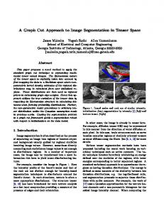
Fig. 1: Illustration of flow passing through t-links (right) for segmenting a 2D image (left). some terminology. In accordance with the graph construction given in [9], we consider (without loss of generality) that a node is linked to at most one terminal, i.e : (s, p) ∈ Et ⇒ (p, t) 6∈ Et

3. REDUCING GRAPHS As we have seen before, the memory usage for segmenting high-resolution data by graph cuts can be prohibitive. As an illustration, the max-flow algorithm of Boykov and Kolmogorov [6] (version 2.2) allocates 24|P| + 14|En | bytes. In table 1, we observe that for a fixed amount of RAM, the maximum volume size decreases quickly as dimension d increases. Nevertheless, we observe on figure 1 that most of the nodes are useless because not traversed by any flow. On the right hand-side of figure 1, we represent the flow passing through the t-links. Light gray pixels (respectively dark gray pixels) indicates that a strictly positive amount of flow is passed from s to node p (respectively from node p to t). Clearly, only a small part of nodes is used during the max-flow computation. When reducing such a graph, one would like extract the smallest possible graph G 0 = (V 0 , E 0 , c) from G while keeping a 1 Typically, larger neighborhood systems yield better results but increase running times and memory consumptions. 2 An implementation of the max-flow algorithm is freely available at http://www.cs.cornell.edu/People/vnk/software.html

4459 219 45

∀p ∈ P.

Also, we summarize the capacities of the t-links at any node p ∈ P by c(p) = c(s, p) − c(p, t). For any B ⊂ Zd and ex the set translation of B by the point x ∈ P, we denote by B e x : Bx = {b+x | b ∈ B}. Moreover, for Z ⊂ P and B ⊂ Zd , we define the dilation of Z by B as : [ ez . ZeB = {z + b | b ∈ B, z ∈ Z} = B z∈Z

We also define, for any Z ⊂ P, the maximal amount of flow coming in and out through the n-links by P P Pin (Z) = p∈Z,q6∈Z c(p, q), Pout (Z) = p∈Z,q6∈Z c(p, q). p∈N (q)

q∈N (p)

Finally, we define the maximum amount of flow passing through the t-links and the flow orientation by X X A(Z) = |c(p)|, O(Z) = sign(c(p)), p∈Z

p∈Z

where sign(t) = 1 if t > 0, 0 if t = 0 and −1 otherwise.

Let B ⊂ Zd , in order to build G 0 , we remove from the nodes of G any Z ⊂ P such that either eB ) = +|Z eB | and A(ZeB \ Z) ≥ Pout (Z eB ), or O(Z e e e e O(ZB ) = −|ZB | and A(ZB \ Z) ≥ Pin (ZB ).

(2)

hal-00522302, version 1 - 30 Sep 2010

As an illustration of those conditions, notice for instance that the last condition implies that all the flow that might come in the region ZeB comes from its boundary and can be absorbed eB \ Z. Building such sets Z is done by testing by the band Z each individual pixels of Z. In order to do so, we establish (in a forthcoming paper) that the conjonction of conditions (2) for every z ∈ Z implies (2) for Z. Considering B, a square window of size (2r + 1) (r > 0) centered at the origin, a more conservative test for z ∈ Z is ( ez c(q) ≥ +δ · γ ∀q ∈ B or (3) ez , c(q) ≤ −δ · γ ∀q ∈ B where γ ∈ [0, 1] and δ =

P (B) (2r+1)2 −1 ,

with

P (B) = max(|{(p, q), p ∈ Z, q 6∈ Z and p ∈ N (q)}|, |{(p, q), p ∈ Z, q 6∈ Z and q ∈ N (p)}|). If all the capacities of the n-links are smaller than 1 (which is true for most interesting energies) and (3) holds, the inegality (2) holds for Z = {z}. Then, G 0 is determined by the set of nodes V 0 = {p ∈ P not satisfying (3)} ∪ {s, t}. We have theoretical and empirical evidence suggesting that this graph reduction provides an exact solution when γ = 1. It becomes an heurisitic as γ decreases to 0. Morever, the condition (3) is simple and a straightforward implementation has a worstcase complexity of O(|B|). Decomposing this test along the d dimensions yields an algorithm with complexity O(1), except for image borders. 4. EXPERIMENTAL RESULTS This section compares the performance of standard graph cuts and our method in terms of speed, memory and segmentation accuracy with two energy models : T V + L2 [10] and Boykov/Jolly [8]. Experiments are performed on an Athlon Dual Core 6000+ 3GHz with 2GB RAM for segmenting 2D/ 3D images in connectivity 1. Times are averaged over 10 runs. 4.1. T V + L2 energy model Total variation has originally been introduced by Rudin et al. for image denoising. The authors of [10] have proposed to use the T V + L2 model for image segmentation. First, the middle row of figure 2 describes the influence of the window parameter r. For r = 0, time and memory usage correspond to standard graph cuts. The general trend is that the amount of allocated memory first decreases and then increases as r increases. This corresponds to the fact that in (3), each individual test |c(q)| ≥ δ is easier to satisfy when r is

large, because δ decreases with r. However, the test on the signs are more difficult to satisfy since the window is larger. Note that the value of r which minimizes the memory usage depends both on the image structure and the model’s parameters. Except for the image « plane », our algorithm is generally faster than standard graph cuts. Second, figure 2 also illustrates the role of the γ parameter. The window radius is chosen to minimize both normalized time and memory usage. The differences between the reference and the segmentation are evaluated using the Dice Similarity Coefficient (DSC) and the Hausdorff distance 3 . For all images, the memory usage can be significantly reduced by lowering the γ parameter while getting nearly the same solution up to a certain value. 4.2. Boykov and Jolly’s energy model Introduced in [8], this model has quickly become a standard in applications. From a user viewpoint, it consists of marking some parts of the image as « object » and « background ». For more information, we refer the reader to [8]. Figure 3 compares time and memory usage between standard graph cuts and our method for segmenting real images. The second image represents a simulated brain MRI generated by Brainweb with 3% of noise 4 while the third image shows an abdominal CT with a pulmonary tumor. In these experiments, the model’s parameters are optimized for better visualization while γ parameter is set to 1. The window radius is chosen such that memory usage is minimized. Seeds were placed by hand but are not represented here because space limitations. For all images, the amount of allocated memory for the graph is reduced by a factor ranging from 4.8x to 7.7x. For the first image, our algorithm is 1.7x faster and require 4.8x less memory while getting exactly the same result. Moreover, altough the graphs induced by the volumes « brain » and « ct-thorax » do not fit in memory when no reduction is performed, we observe that our algorithm is able to segment them in less than 10 seconds. 5. REFERENCES [1] Yin. Li, Jian. Sun, Chi-Keung. Tang, and Heung-Yeung. Shum, “Lazy snapping,” ACM Transactions on Graphics, vol. 23, no. 3, pp. 303–308, 2004. [2] A.K. Sinop and L. Grady, “Accurate banded graph cut segmentation of thin structures using laplacian pyramids,” in MICCAI, 2006, vol. 9, pp. 896–903. [3] H. Lombaert, Y.Y. Sun, L. Grady, and C.Y. Xu, “A multilevel banded graph cuts method for fast image segmentation,” in ICCV, 2005, vol. 1, pp. 259–265. 3 Details on these evaluation measures are available at http://lts08.bigr.nl/about.php 4 The Brainweb simulator is freely accessible at http://mouldy.bic.mni.mcgill.ca/brainweb/

hal-00522302, version 1 - 30 Sep 2010

(a) plane – 1443 × 963

(b) cells – 1536 × 1536

(c) lena – 2048 × 2048

(d) woman – 211 × 172 × 92

(e) Image « plane »

(f) Image « cells »

(g) Image « lena »

(h) Image « woman »

(i) Image « plane »

(j) Image « cells »

(k) Image « lena »

(l) Image « woman »

Fig. 2: Influence of window radius (middle row) and γ parameter (bottom row) for segmenting 2D/3D images (top row) with a T V + L2 energy model. On the two last rows, blue curve with squares and red curve with triangles correspond respectively to time execution and amount of memory allocated by the graph. On bottom row, green curve with circles and purple curve with diamonds correspond respectively to the DSC and the Hausdorff distance between normal and γ-parametrized segmentations. maximum a posteriori estimation for binary images,” Journal of the Royal Statistical Society, vol. 51, no. 2, pp. 271–279, 1989.

(a) book – 3012 × 2048

Image book brain ct-thorax

(b) brain – 181 × (c) ct-thorax – 245 × 217 × 181 245 × 151

Original Time Memory 5.58 1.08 Gb / 3.59 Gb / 4.58 Gb

Our algorithm Time Memory 3.25 231.25 Mb 9.02 734.64 Mb 8.25 606.27 Mb

Fig. 3: Speed (secs) and memory usage compared to standard graph cuts for segmenting 2D/3D images (top) with a Boykov/Jolly’s energy model [8].

[4] C. Cigla and A.A. Alatan, “Region-based image segmentation via graph cuts,” in ICIP, 2008, pp. 2272– 2275. [5] D. M. Greig, B. T. Porteous, and A. H. Seheult, “Exact

[6] Y. Boykov and V. Kolmogorov, “An experimental comparison of min-cut/max-flow algorithms for energy minimization in vision,” IEEE Transactions on PAMI, vol. 26, no. 9, pp. 1124–1137, 2004. [7] A. Delong and Y. Boykov, “A scalable graph-cut algorithm for n-d grids,” in CVPR, 2008, pp. 1–8. [8] Y. Boykov and M-P. Jolly, “Interactive graph cuts for optimal boundary and region segmentation of objects in n-d images,” in ICCV, 2001, vol. 1, pp. 105–112. [9] V. Kolmogorov and R. Zabih, “What energy functions can be minimized via graph cuts ?,” IEEE Transactions on PAMI, vol. 26, no. 2, pp. 147–159, 2004. [10] F. Ranchin, A. Chambolle, and F. Dibos, Total Variation Minimization and Graph Cuts for Moving Objects Segmentation, pp. 743–753, 2007. [11] L. Dice, “Measure of the amount of ecological association between species,” Ecology, vol. 26, no. 3, pp. 297–302, 1945.