Parameter Selection for Graph Cut Based Image Segmentation∗ Bo Peng†
Olga Veksler
[email protected]
[email protected]
Hong Kong Poltechnic University Hung Hom, Kowloon, Hong Kong
University of Western Ontario London, ON N6A 5B7 Canada
Abstract
The graph cut based approach has become very popular for interactive segmentation of the object of interest from the background. One of the most important and yet largely unsolved issues in the graph cut segmentation framework is parameter selection. Parameters are usually fixed beforehand by the developer of the algorithm. There is no single setting of parameters, however, that will result in the best possible segmentation for any general image. Usually each image has its own optimal set of parameters. If segmentation of an image is not as desired under the current setting of parameters, the user can always perform more interaction until the desired results are achieved. However, significant interaction may be required if parameter settings are far from optimal. In this paper, we develop an algorithm for automatic parameter selection. We design a measure of segmentation quality based on different features of segmentation that are combined using AdaBoost. Then we run the graph cut segmentation algorithm for different parameter values and choose the segmentation of highest quality according to our learnt measure. We develop a new way to normalize feature weights for the AdaBoost based classifier which is particularly suitable for our framework. Experimental results show a success rate of 95.6% for parameter selection.
1 Introduction General purpose image segmentation is a highly ambiguous problem. In many applications, such as medical imaging, user guidance is available to help reduce the ambiguities in segmentation. Sometimes, even with a small amount of user interaction, segmentation quality is largely improved. Thus interactive segmentation techniques are becoming increasingly popular over the last decade. In this paper we consider the most common type of interactive segmentation: segmentation of the object of interest from its background. There are many different approaches to interactive segmentation, such as snakes [9], livewire [6], and level sets [14]. In recently years, interactive segmentation based on a graph cut [3, 4] has become very popular. The original work is due to Boykov and Jolly [3], followed by extensions [1, 12, 18]. Probably the biggest advantage of the graph ∗ This † This
work was partially supported by NSERC Canada work was done while Bo Peng was a student at the University of Western Ontario.
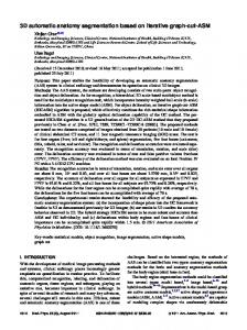
(a)
(b) λ = 2
(c) λ = 10
(d) λ = 18
(e) λ = 26
(f) λ = 34
(g)λ = 42
(h) λ = 50
Figure 1: (a) is the original image with the seeds; (b-h) show the object segment for an increasing value of parameter λ ; (b,c) are oversegmentations, (d,e) are good segmentations, and (f-h) are undersegmentations. cut algorithm is that it addresses segmentation in a global optimization framework and guarantees a globally optimal solution for wide class of energy functions [11]. Another advantage is that both the regional and the boundary properties can be used. In addition, the user interface is simple and convenient - the user marks some object and background ”seeds”. The seeds can be loosely positioned inside the object and background regions, which is easier compared to placing seeds exactly on the boundary, like in livewire [6]. A fundamental, but far from having been solved issue in graph cut segmentation is parameter selection. Inappropriate choice of parameters may result in unsatisfactory segmentation, and the user may have to spend a significant amount of time correcting the segmentation. In this paper, we address selecting one of the most important parameters in graph cut segmentation, which we call parameter λ (see Sec. 2). Fig. 1 (b-h) shows the results of segmenting the image in Fig. 1(a) under different values of λ . The parameter λ controls under/over segmentation of an image. Here, oversegmentation means that the boundary between the object and background regions is too long. In oversegmentation, the object region is not coherent, i.e. it consists of too many pieces or its boundary is not smooth, see Fig. 1(b,c). Undersegmentation means that the boundary between the object and background segments is too short. In undersegmentation, the boundary is too smooth and the background segment may contain pieces of the foreground (or vice versa), see Fig. 1(f-h). For low values of λ , an oversegmentation, and for larger values of λ , an undersegmenation tend to occur. There is a good range of λ values where neither undersegmentation no oversegmentation occurs (Fig. 1(d,e)), however, for each particular image, the range of appropriate λ values may be different [10]. Usually, λ is fixed to a certain value by the developers of the segmentation algorithm, and it is expected to give satisfactory segmentations for the images similar to those that were used to tune the parameters. But when given a different class of images, the results might not be satisfactory. For better performance, λ has to be estimated for each image separately. Statistical approaches, such as [20] lead to computationally intractable estimators. We pursue an empirical approach. Given segmentation results for different λ values, such as in Fig. 1, we choose the best one, according to the measure of segmentation quality that we develop.
We investigate different measures of segmentation quality proposed previously, and develop a measure similar to [15]. Our measure of segmentation quality is based on intensity, gradient, contour continuity, and texture features. We approach the problem of segmentation quality as a binary classification problem (good segmentation vs. bad segmentation), and train a classifier using the AdaBoost algorithm [7]. The idea of selecting parameters based on a segmentation quality measure is not novel, although our particular segmentation quality classifier is novel. The novelty of our work comes from a new way to normalizing feature weights used for the classifier. Our approach to feature normalization is uniquely appropriate for the parameter selection problem, and leads to a big improvement in performance, from error rate of approximately 15% with standard feature normalization to only 4.4% error rate with our normalization. There are several reasons why we address selection of only a single parameter λ . First of all, this parameter has the greatest effect on segmentation results, yet it is the hardest parameter to estimate from the image itself, because it is related to the length of the expected boundary between the object/background regions. Other parameters in the graph cut framework can be reasonably well estimated from the given image. The other reason is computational, since we have to re-run the graph cut algorithm for different parameter values. Therefore the parameter search space has to be low-dimensional. Our training set consists of 80 images with 10 segmentations each, under different λ settings. Segmentations were manually labeled into two classes, ”good” (positive), and ”bad” (negative). Leave one out cross validation error rate is 4.4%, namely the top quality segmentation chosen for an image is a ”bad” segmentation in only 4.4% of cases.
2 Interactive segmentation with a graph cut We now review the interactive segmentation framework of [3]. Segmentation of an object from the background is formulated as a binary labeling problem. Given a set of labels L and a set of pixels P, the task is to assign to each pixel p ∈ P a label f p ∈ L . For binary image segmentation, the label set is L ={0, 1}, where 0 corresponds to the background and 1 corresponds to the object. Let f = { f p | f p ∈ L } stand for a labeling, i.e. label assignments to all pixels. An energy function is formulated as: E( f ) =
∑
D p( f p ) + λ ·
p∈P
∑
w pq · I ( f p 6= fq )
(1)
(p,q)∈N
The first sum in Eq. (1) is called the data term and it measures how pixels like the labels in labeling f . D p ( f p ) measures how well label f p fits pixel p. A common approach, and the one we use in our work, is to build a foreground and background intensity models from the foreground seeds and background seeds, respectively. Then the D p ( f p ) terms are the negative log likelihoods of the constructed background/foreground models. The second sum in Eq. (1) is called the smoothness term and it counts the weighted sum of discontinuities in f . Here I ( f p 6= fq ) is 0 if f p = fq and 1 otherwise. N is a neighborhood system, we use the 4-connected grid which consists of ordered pixel pairs (p, q). The smoothness term prefers a labeling f which does not have many jumps between labels 0 and 1, that is a labeling f is expected to have shorter boundaries between regions labeled as 1 and 0. To encouraged the boundary to lie on the intensity edges in the image, a common choice ([3]) is w pq = e
(I −I )2 − p 2q 2σ
, where I p is the intensity of pixel p.
Parameter σ is related to the level of variation in the image, and it is set to the average absolute intensity difference between the neighboring pixels. Boykov et.al. [3] show how to minimize this energy in Eq. (1) with a minimum cut on a certain graph. We use the efficient algorithm of [2] for computing the minimum cut. The parameter λ in the energy in Eq. (1) controls the relative weight of the data term versus the smoothness term. If λ is too small, an oversegmentation of an image tends to occur. If λ is too large, an undersegmentation typically occurs. Choosing an appropriate λ is a challenging task, and is the main goal of this paper.
3 Segmentation Evaluation Segmentation evaluation is closely tied to the question of what is a good segmentation. While evaluating segmentation results is an important task in itself, in this paper, segmentation evaluation is a crucial task since it forms an integral part of the proposed parameter selection method. See [21] for a review of segmentation evaluation. Many algorithms evaluate segmentation subjectively. Other algorithms use ground truth for evaluation, this is called supervised segmentation evaluation [13, 16]. Supervised evaluation is appropriate if the goal is to compare different segmentation algorithms or to find the best fixed parameters for a single segmentation algorithm. Our goal is to tune λ for each particular image, and thus no ground truth is available. Unsupervised evaluation methods do not rely on ground truth. Heuristics for measuring segmentation quality are designed. The heuristics are based on some cues related to the Gestalt grouping principles, such as intra-region uniformity, inter-region contrast, etc. Many methods design segmentation evaluation heuristically, a review is in [5]. No single cue is enough for a successful segmentation evaluation, therefore multiple cues have to be combined. Cue combination is challenging to address heuristically. Another unsupervised evaluation approach is based on learning an evaluation function from a database with ground truth [15, 19]. Just as the unsupervised approaches, the method in [15] is based on computing different features or statistics on segmentation results. However, the advantage of [15] is that a combination of different features is done in a principled manner, through training a classifier on a hand-segmented database. Our approach to segmentation evaluation is inspired by [15]. In [15], they formulate the problem of determining whether a segmentation is good as binary classification. They train a linear classifier, which given an image and its segmentation, returns 1 if the segmentation is good and -1 otherwise. For training images of good segmentations, they use images segmented by humans [15]. For bad segmentations, they randomly pair a human segmentation with a different image (not the image where this segmentation came from). Their features are computed from ”superpixels” provided by image oversegmentation. We also train a classifier h(x) to recognize a good segmentation. Our training data consists of segmentation results under different values of λ . We manually label good segmentations as positive examples, and bad segmentations (undersegmentation and oversegmenation) as negative examples. Our training data is harder than in [15]. In [15], the negative examples are created by pairing a segmentation provided by a human with a random image. Therefore, even though segment boundaries are smooth, there is no contrast on the boundary and no coherency inside regions, in most cases. The good segmentations (positive examples) have a good contrast on the boundary. Therefore it should be
relatively easy to separate the two classes, and, in fact, [15] find that a linear classifier is sufficient. In our training set, all segmentations are produced by the graph cut algorithm for different values of λ , and all of them tend to have segment boundaries coinciding with intensity edges in the image, which makes our classification problem harder. An input to the classifier h(x) is a feature vector x which consist of features extracted from a segmentation example. We discuss the features that we use in Sec. 4. Unlike [15], we did not find it necessary to compute ”superpixels” to base our features on. We use the Real AdaBoost [7] to train a classifier h(x). Real AdaBoost, in addition to the class label, provides confidence estimates, c(x). A high positive value of c(x) indicates that the classifier is very confident that x is in the positive class (i.e. a good segmentation). Thus instead of just a binary decision, namely a good or a bad segmentation, we take the confidence value c(x) as the final measure of segmentation goodness, which gives a real range of values. We use implementation of [17].
4 Segmentation Features We now describe the features that we use for classifier training. We use features based on intensity, texture, gradient direction, and corners. The features are computed based on the original image I, and its segmentation S. Here I p is the intensity of pixel p, S p = 0 and S p = 1 mean that pixel p is assigned, respectively, to the background or the object. In general, there may be multiple object/background segments. We use gray level images because their segmentation is more challenging compared to color images. Intensity Features One of the most intuitive and frequently used features for quantifying the quality of a segmentation is based on the intra-region uniformity and inter-region dissimilarity. Often in the object region, image pixels might have nearly constant or slowly varying intensity, and the intensity differences between pixels on the boundary of the object and background regions are often greater than the differences within the object region. In the case of images with little texture, these intensity based intra-region and inter region criteria prove to be effective and simple. So we combine two properties for measuring the quality of segmentation: the inter-region differences across the boundary and the intra-region differences between neighboring pixels within each object region1. First intensity feature is based on the pairwise average absolute intensity differences: Fintensity1 (I, S) =
∑(p,q)∈B |I p − Iq | ∑(p,q)∈O |I p − Iq | − |B| |O|
where B is the set of pairs of neighboring pixels along the object boundary, i.e. B = {(p, q)|S p = 1, Sq = 0 or S p = 0, Sq = 1}; O is the set of pairs of pixels inside an object region, i.e. O = {(p, q)|S p = 1, Sq = 1}; |B| and |O| are the sizes of sets B and O, respectively. For a good segmentation, Fintensity1 should be positive and large. We also compare the histogram of absolute intensity differences of pixel pairs in B and the histogram of pixel pairs in O. Their histograms should be distinct. To measure the dissimilarity between the histograms, we use the χ 2 statistic, which is given by: 1 As mentioned before, we assume that there is coherency only within the object region, and therefore we do not measure intra-region similarity within the background region.
Fintensity2 (I, S) = ∑ i
2 ˆ (H(i, B) − H(i)) ˆ H(i)
ˆ = [H(i, B) + H(i, O)]/2 where H(i, X) is the value of the histogram of X at bin i, and H(i) is the mean histogram. Our two intensity based features are based on the assumption that the object has constant or slowly changing intensities. They may be misleading if the object has strong texture, in which case texture features are more helpful, see section below. Gradient Direction Features The gradient of an image is anther important feature. For a good segmentation, we expect the gradient to change smoothly in most places on the boundary, unless the object or background have strong texture. The gradient magnitude is already captured in Fintensity1 and Fintensity2 . However, sometimes there is a weak boundary with very weak gradient ~ magnitude but very consistent gradient direction. Let G(p) be the gradient direction at pixel p. We can capture gradient direction consistency in the following feature: Fgradient1 (I, S) =
~ ~ − G(q)| ∑(p,q)∈B |G(p) , |B|
where, as before, B is the set of pixel pairs on the boundary of background/object regions. Fgradient1 is the average value of gradient direction differences. The smaller it is, the higher is the quality of the extracted boundary. We also have another feature based on gradient direction which is based on variance: q ~ ~ ¯ 2 − G(q)| − G) ∑(p,q)∈B (|G(p) Fgradient2 (I, S) = , |B| where G¯ is the average difference of gradient directions on the boundary. A small value of Fgradient2 indicates a good segmentation. Boundary Corner Feature Smoothness of a boundary is a strong cue for human perception system. Therefore we expect that a good segmentation will have smooth boundaries with only a few corners. We use SUSAN corner detector to detect any corners on the object/background boundary. We detect corners in the ”mask” image M corresponding to segmentation S. That is M p = 0 if S p = 0 and M p = 255 if S p = 1, where M p is the value of image M at pixel p. For the boundary feature, we simply set Fboundary(S) to be the number of corners detected in the segmentation S. Notice that we do not need the original image I for this feature. Texture Feature The last feature we use for our classifier is based on texture. It helps to detect a good segmentation when strong texture is present in the object. A standard way to describe texture
is through a bank of Gabor filters [8]. To compare texture of the object and background, we compute the histograms of Gabor filter bank responses separately for the object and the background. Then we set Ftexture to be the χ 2 distance between these histograms. As a measure of the quality of segmentation, the texture difference between the object and background is expected to be large for a good segmentation and small for a bad one. In the case of undersegmentation, a part of object might be classified as a part of background (or vice versa), thus Ftexture will be small. However, the drawback of this feature is it cannot detect oversegmentation, which may receive a high score under Ftexture .
5 Feature Normalization Before training the classifier, features have to be normalized, since they vary widely across different images and cannot be directly compared. There are two standard ways for feature normalization. First way is used to make sure different features are on approximately the same scale, since this is desirable for some classifiers. Let x1 , x2 , ...xn be the n trainj ing samples, and let the jth feature of ith sample be xi . In such case, if d is the total j j j number of features, then for j = 1, ..., d, jth feature values x1 , x2 , ..., xn are normalized to be approximately in some fixed range, usually in [0, 1] or [−1, 1]. This is done either j j j by linearly stretching the range, or by normalizing values x1 , x2 , ..., xn to have zero mean, unit variance. Such feature normalization has no effect on our AdaBoost classifier. Second way is to normalize each training image itself, for example, by linearly stretching all the intensity values to some fixed range, usually between [−1, 1]. The idea is that any features computed from normalized examples will be roughly in the same range. We found that the standard approach to feature normalization does not work well. The error rate, at best, was around 15% when we tried different ways of normalizing the training images. The reason is as follows. In different images, the average contrast on the boundary between the object of interest and the background can be very different, sometimes only a few gray level values, and sometimes as large as a hundred gray level values. Thus the range of Fintensity1 , Fintesnsity2 and other features values that correspond to a good segmentation varies widely across different images, even after image normalization. Thus there is no single threshold for any of the feature that works reasonably well for any feature, leading to a weak classifier performance. Let I be some image. Recall that we perform segmentation for different λ values. Let S1 , S2 , ..., Sk be the k different segmentations of image I, and let x1 , x2 , ..., xk be the k training examples2 corresponding to these segmentations. Let J be another image and y1 , y2 , ..., yk be the k training examples corresponding to the k segmentations of image J. j j For these examples, let us consider the values of some fixed feature j, that is x1 , x2 , j j j j ..., xk for image I and y1 , y2 , ..., yk for image J. Suppose the jth feature corresponds to Fintensity1 , so the larger the feature value, the better is the separation between the object and the background. The range of xij ’s maybe between (0.1, 0.4) and the range of yij ’s between (0.3, 0.7). Due to the contrast differences in the images I and J, a value of 0.3 most likely signals a good segmentation for image I, but not a good segmentation for image J. Therefore, for image I, we should care about how large the values of xij are compared to the range of values in x1j , x2j , ..., xkj , that is compared to the other values 2 Each training example x corresponds to a vector of features extracted from image I and segmentation S . i k The features are as described in Sec. 4.
in its own range. In other words, we do not care about the absolute values of features x1j , x2j , ..., xkj , but only about their rank in relation to each other. So our feature normalization is as follows. Given k examples (feature vectors) x1 , x2 , ..., xk corresponding to the k segmentations of an image I under different λ settings, for each feature j, we replace xij with its rank in the set {x1j , x2j , ..., xkj }. We found this normalization to be very effective, see Sec. 6. Our feature normalization is uniquely suitable for the parameter selection problem, since for a given image, we normalize feature values with respect to all segmentations for this image. Therefore, our measure of segmentation quality can only be applied to a set of segmentation results for a single image, i.e. it cannot be applied to a single segmentation, and therefore it is not a stand-alone measure like the one in [15].
6 Experimental Results We have collected 80 images of natural scenes from the web, and performed graph cut segmentation with λ in the range from of 2 to 74 with a step size of 8, which gives 10 segmentation results per image. We manually labeled each segmentation result as ”good” (the positive class) or ”bad” (the negative class). Currently, our system is applied after the user enters all the brush strokes. The system could be rerun after user makes corrections. Since our data set is small, we use leave one out cross validation (LOOCV). We take one image out of 80 (which means that we take out all 10 segmentations for different values of λ for this image) and train the classifier on the remaining 79 images. Then we test the classifier on the image (all the 10 segmentation associated with it) we took out. If we compute the overall classification error (bad segmentations classified as good, and vice versa), it is 16.1%. However, our goal is to return to the user the segmentation result which we think is the best one, therefore we measure error rate differently. Out of 10 segmentation results for the image that was held out, we return to the user the segmentation with the highest confidence value for being in the positive class. Now the natural measure of error is how many bad segmentations are returned to the user, that is how often the segmentation with the highest confidence for being a good segmentation is actually a bad segmentation. The error rate is only 4.37%. Our new feature normalization scheme makes a big difference in results. If we use a standard normalization approach, the error rate is around 15%, where, again, the error is measured as the percentage of bad segmentations returned to the user (the overall classification error rate is worse than 30%). We also test how well our parameter selection works compared to using a fixed λ . We perform segmentation with a fixed value of λ in the range from 2 to 114 in step size of 8. For each fixed λ , we compute the error rate, that is the percentage of bad segmentations. The error rate starts at 100% for λ = 2, then goes down to 39.5% for λ = 66 and then goes up again to 83.9% for λ = 114. Thus if segmentation with a fixed λ is performed, the best error rate would be 39.5%, which is significantly worse compared to choosing an appropriate λ using our system. Some randomly chosen results for automatically selecting parameter λ are in figure 2. The average running time to perform graph cut segmentation, compute the features, and classify the results is under 3 minutes. To improve efficiency, we could use the parametric max flow algorithm of [10], which allows computing the series of minimum cuts corresponding to different values of λ with only slight increase in cost compared to com-
puting a single cut. Note however, that the majority of time for our algorithm is spent on computing features, thus the speedup would be relatively modest.
References [1] A. Blake, C. Rother, M. Brown, P. Perez, and P.H.S. Torr. Interactive image segmentation using an adaptive gmmrf model. In ECCV, pages Vol I: 428–441, 2004. [2] Y. Boykov and V. Kolmogorov. An experimental comparison of min-cut/max-flow algorithms for energy minimization in vision. TPAMI, 26(9):1124–1137, 2004. [3] Yuri Boykov and M. P. Jolly. Interactive graph cuts for optimal boundary and region segmentation. In ICCV, volume I, pages 105–112, 2001. [4] Y.Y. Boykov and G. Funka Lea. Graph cuts and efficient n-d image segmentation. International Journal of Computer Vision, 69(2):109–131, September 2006. [5] S. Chabrier, B. Emile, H. Laurent, C. Rosenberger, and P. Marche. Unsupervised evaluation of image segmentation application to multi-spectral images. In ICPR, pages 576–579, 2004. [6] A. X. Falaco, J.K. Udupa, S. Samarasekara, and S. Sharma. User-steered image segmentation paradigms: Live wire and live lane. In Graphical Models and Image Processing, volume 60, pages 233–260, 1998. [7] Yoav Freund and Robert E. Schapire. A decision-theoretic generalization of on-line learning and an application to boosting. J. Comput. Syst. Sci., 55(1):119–139, 1997. [8] S.E. Grigorescu, N. Petkov, and P. Kruizinga. Comparison of texture features based on gabor filters. TIP, 11(10):1160–1167, 2002. [9] M. Kass, A. Witkin, and D. Terzopoulos. Snakes: Active contour models. IJCV, 2:321–331. [10] V. Kolmogorov, Y.Y. Boykov, and C. Rother. Applications of parametric maxflow in computer vision. pages 1–8, 2007. [11] Vladimir Kolmogorov and Ramin Zabih. What energy function can be minimized via graph cuts? TPAMI, 26(2):147–159, February 2004. [12] Y. Li, J. Sun, C.K. Tang, and H.Y. Shum. Lazy snapping. ACM Trans. Graph., 23(3):309–314. [13] David R. Martin, Charless Fowlkes, Doron Tal, and Jitendra Malik. A database of human segmented natural images and its application to evaluating segmentation algorithms and measuring ecological statistics. In ICCV, pages II: 416–423, 2001. [14] S. Osher and J.A. Sethian. Fronts propagating with curvature dependent speed: Algorithm based on hamilton jacobi formulations. Journal of Computational Physics, 79:12–49, 1988. [15] X. Ren and J. Malik. Learning a classification model for segmentation. In ICCV, volume 1, pages 10–17, 2003. [16] R. Unnikrishnan, C. Pantofaru, and M. Hebert. Toward objective evaluation of image segmentation algorithms. PAMI, 29(6):929–944, 2007. [17] A. Vezhnevets. http://research.graphicon.ru/machine-learning/gml-adaboost-matlab- toolbox.html. [18] S. Vicente, V. Kolmogorov, and C. Rother. Graph cut based image segmentation with connectivity priors. In CVPR, page to appear, 2008. [19] Hui Zhang, Sharath Cholleti, Sally A. Goldman, and Jason E. Fritts. Meta-evaluation of image segmentation using machine learning. In CVPR, pages 1138–1145, 2006. [20] Li Zhang and Steven M. Seitz. Estimating optimal parameters for mrf stereo from a single image pair. TPAMI, 29(2):331–342, February 2007. [21] Y.J. Zhang. A review of recent evaluation methods for image segmentation. ISSPA, 1:148– 163, 2001.
Figure 2: Segmentation results produced by automatically selecting λ .