Refining neural network predictions for helical ... - CiteSeerX

Refining neural network predictions for helical transmembrane proteins by dynamic programming Burkhard Rost ◊, EMBL, 69012 Heidelberg, Germany EBI, Hinxton, Cambridge CB10 1RQ, U.K. [email protected] Abstract For transmembrane proteins experimental determina-tion of three-dimensional structure is problematic. However, membrane proteins have important impact for molecular biology in general, and for drug design in particular. Thus, prediction method are needed. Here we introduce a method that started from the output of the profile-based neural network system PHDhtm (Rost, et al. 1995). Instead of choosing the neural network output unit with maximal value as pre-diction, we implemented a dynamic programming-like refinement procedure that aimed at producing the best model for all transmembrane helices compatible with the neural network output. The refined prediction was used successfully to predict transmembrane topology based on an empirical rule for the charge difference between extra- and intra-cytoplasmic regions (posi-tive-inside rule). Preliminary results suggest that the refinement was clearly superior to the initial neural network system; and that the method predicted all transmembrane helices correctly for more proteins than a previously applied empirical filter. The resul-ting accuracy in predicting topology was better than 80%. Although a more thorough evaluation of the method on a larger data set will be required, the results compared favourably with alternative methods. The results reflected the strength of the refinement procedure which was the successful incorporation of global information: whereas the residue preferences output by the neural network were derived from stretches of 17 adjacent residues, the refinement procedure involved constraints on the level of the entire protein.

Rita Casadio, and Piero Fariselli Lab. of Biophysics, Dep. of Biology Univ. of Bologna, 40126 Bologna, Italy [email protected]

Introduction Given the rapid advance of large-scale genesequencing projects (Fleischmann, et al. 1995), most protein sequences of key organisms will probably be known in a few years' ◊ Corresponding author. Abbreviations: 3D, three-dimensional; HTM, transmembrane helix (also abbreviated by H in figures, L used for nontransmembrane regions); PDB, Protein Data Bank of experimentally determined 3D structures of proteins; PHDhtm, Profile based neural network prediction of helical transmembrane regions; SWISS-PROT, data base of known protein sequences.

time. Currently, the gap between the number of known protein sequences and protein threedimensional (3D) structures is still increasing (Rost 1995). However, experimental structure determination is becoming more of a routine (Lattman 1994). Thus, within the next decades we may know the three-dimensional (3D) structure for most proteins. Even in such an optimistic scenario, experimental information is likely to remain scarce for integral membrane proteins. These challenge experimental structure determination: X-ray crystallography is problematic as the hydrophobic molecules hardly crystallise; and for nuclear magnetic resonance (NMR) spectroscopy transmembrane proteins are usually too long. Today, 3D structure is known for only six membrane proteins (Rost, et al. 1995). Can theory predict structural aspects for integral membrane proteins? Theoretical predictions for helical transmembrane proteins. The prediction of structural aspects is simpler for membrane proteins than for globular proteins as the lipid bilayer imposes strong constraints on the degrees of freedom of 3D structure (Taylor, et al. 1994). Most prediction tools focus on helical transmembrane proteins for which some experimental information about 3D structure is

available (Manoil & Beckwith 1986, Hennessey & Broome-Smith 1993). Methods have been designed to predict the locations of transmembrane helices

better prediction of topology require to predict more accurately each residue (per-residue

Input: topology: out N

extracytoplasmic lipid bilayer of membrane

search align predict predict similar homologues preferences locations sequences BLAST

N topology: in

intracytoplasmic

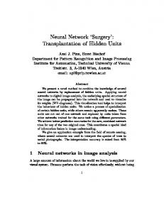
Fig. 1. Definition of topology. In one of the two known classes of membrane proteins, typically apolar helices are embedded in the lipid bilayer oriented perpendicular to the membrane surface. The helices can be regarded as more or less rigid cylinders. 'Topology' is defined as out when the N-term (first residue) starts on the extra-cytoplasmic side and as in if it starts on the intra-cytoplasmic side.

(Kyte & Doolittle 1982, Engelman, et al. 1986, von Heijne 1986, von Heijne 1992, Edelman 1993, Jones, et al. 1994, Persson & Argos 1994, Donnelly & Findlay 1995), and the orientation of transmembrane helices with respect to themembrane (dubbed topology, Fig. 1; (von Heijne 1986, Hartmann, et al. 1989, von Heijne 1989, Sipos & von Heijne 1993, Jones, et al. 1994, Casadio & Fariselli 1996). If the transmembrane helix locations and topology are known with sufficient accuracy, 3D structure can be successfully predicted for the membrane spanning segments by an exhaustive search of the entire structure space (Taylor, et al. 1994). Further improvement of prediction accuracy necessary?. There are two incentives to aim at improving the accuracy of predicting transmembrane helix locations. (1) In general, current prediction methods are probably not accurate enough to be used for the 3D prediction proposed by Taylor and colleagues (Taylor, et al. 1994). (2) A simple means to predict topology (Fig. 1) is the positive-inside rule: positively charged residues are abundant in periplasmic loops of membrane proteins (von Heijne 1986, von Heijne & Gavel 1988, Hartmann, et al. 1989, Boyd & Beckwith 1990, von Heijne 1992). To successfully apply this rule, a correct prediction of the nontransmembrane regions is required. Would a

helical membrane protein sequence of unknown helix location

MaxHom

PHDhtm

PHDhtm filter

Intermediate output: preferences for each residue to be in a transmembrane helix

Fig. 2. Neural network predictions for transmembrane helix preferences (PHDhtm). Input was a protein sequence; output were the locations of transmembrane helices. (1) Similar sequences were searched for in SWISS-PROT (Bairoch & Boeckmann 1994) by the fast alignment algorithm BLAST (Altschul, et al. 1990)). (2) The resulting sequences were realigned by the multiple alignment algorithm MAXHOM (Sander & Schneider 1991) . (3) Profiles derived from the alignment were input into the neural network system PHDhtm (Rost, et al. 1995) . (4) The final output of PHDhtm were the locations of transmembrane helices assigned according to the output unit with maximal value (winner-takes-all).

accuracy), or would it suffice to predict more trans-membrane helices correctly (per-segment accuracy; (Rost, et al. 1994, Rost, et al. 1995)? Here we introduce a conceptually simple method that started from the output of the profile-based neural network system PHDhtm (Fig. 2). The preferences for residues to be in transmembrane helices output from the neural network system were post-processed by a dynamic programming-like algorithm. A similar algorithm has been used before to improve statistics-based predictions for transmembrane helices (Jones, et al. 1994). The algorithm constitutes an example for a problem-specific improvement of neural network output. The resulting predictions were used to predict topology based on charge differences between extra- and intra-cytoplasmic residues (Fig. 1). The method is described in detail; and some preliminary results are given.

Database and evaluation of method

Selection of proteins. We based our analyses on a set of 68 proteins for which experimental information about the locations of transmembrane helices is annotated in the SWISS-PROT database (von Heijne 1992, Bairoch & Boeckmann 1994). The locations of transmembrane helices used are listed in our previous work (Rost, et al. 1995). The observed topology was taken from SWISS-PROT or (Jones, et al. 1994)(Jones, et al. 1994; names listed in Table 2). Note that the set was the same as used previously (Rost, et al. 1995), except for melittin, that was excluded for the purpose of topology prediction. Cross-validation test. For the prediction of transmembrane propensities by the neural network system (PHDhtm; (Rost, et al. 1995), the set of 68 transmembrane proteins (Table 2) was divided into 55 proteins used for training the networks and 13 used for deriving the propensities (test set). This was repeated five times (five-fold cross-validation) such that each protein was in one test set. The sets were chosen such that no protein in the multiple alignments used for training the networks had more than 25% pairwise sequence identity to any protein in the multiple alignments of the proteins for which the propensities were predicted. The crossvalidation procedure yields estimates for prediction accuracy that are likely to hold for proteins of yet unknown topology (Rost & Sander 1993, Rost & Sander 1995, Rost & Sander 1996). Measuring prediction accuracy. We compiled results for per-residue scores capturing the accuracy of predicting HTM placement (Table 1); and per-segment scores capturing the accuracy of predicting entire HTM's correctly. Due to the length of HTM's and the prediction accuracy, the definition of segment-based scores was straightforward (in contrast to the case of secondary structure predictions for globular proteins (Rost, et al. 1994)). We regarded a transmembrane helix to be predicted correctly, if the overlap between observed and predicted helix was at least five residues (Table 1). Furthermore, we compiled the percentage of proteins for which all HTM's were correctly

Post-processing neural network output by dynamic programming

Neural network predictions of HTM propensities. Our previously published prediction tool PHDhtm (Rost, et al. 1995) uses multiple sequence alignments as input to a neural network system (Fig. 2). The network output are two values for each residue, describing the propensity of that residue to be in a transmembrane helix (H) or to be in a region outside of the lipid bilayer (L). We used two levels of networks: a first sequence-to-structure level and a

Input: neural network output, i.e., preference for each residue: HTM / non-HTM Convert preferences to propensities Generate pool with all possible HTM's Compile average propensity for HTM Find HTM µ with maximal propensity Add segment µ to model Compile score over all residue propensities for model with µ HTM's loop

Materials and methods

predicted (QM) and the percentage of proteins for which topology was correctly predicted (Q T). Note: the topology prediction was regarded as correct if and only if all HTM's and the orientation of the HTM's with respect to the membrane were correctly predicted.

Score for model µ > score for model µ - 1 ? yes

exclude HTM µ and all overlapping HTM's from pool

no terminate ! final prediction: model µ -1

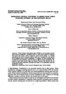
Output: number and locations of best model, i.e., predicted HTM's Fig. 3. Flow chart for refinement algorithm. Input to the refinement are the PHDhtm preferences for each residue to be in the HTM or in the non-HTM state. Output are the predictions of the number and locations of all segments in the protein.

second structure-to-structure level (Rost 1996). The second level captures correlations between adjacent residues, i.e., learns to regard transmembrane helices as objects of a minimal length. The effect of the second level is an increase in the average length of a predicted helix. However, the second level frequently predicts too long helices. We previously corrected this by introducing an empirical filter (PHDhtm filter) that relied crucially on choosing free parameters (Rost, et al. 1995). Finding the optimal path through all predicted propensities (dynamic programming). The simplest way to obtain predictions for HTM locations from propensities is to predict each residue to be in the state (H or L) with largest propensity. An alternative for generating predictions from propensities is an algorithm similar to dynamic programming which has been investigated for predicting transmembrane topology by Jones, Taylor and Thornton (Jones, et al. 1994). The main purpose of this algorithm, as we implemented it, was to generate the optimal placements of HTM segments compatible with the neural network output. The network residue preferences were derived from information largely local in sequence (input to neural network: profiles for 17 adjacent residues). The refinement involved using information about the entire protein, and hence, the procedure - to some extent - made use of global information. The refinement was implemented by the following four steps (Fig. 3). (1) Converting neural network output to propensities. The residue preferences output by PHDhtm were converted to residue propensities p , normalised to sum to one for each residue: H oi H pi = H L and piL = 1 - pH i , for i = 1, .., Nres( oi +oi 1) where Nres was the number of residues (protein length), o iH and o Li the values of the network output unit coding for the HTM and the nonHTM state of residue i . (2) Compiling average propensity for all possible transmembrane helices. The average propensity for all possible HTM's T were compiled by summing the HTM propensities over all residues of T :

i+Lm-1 1 pH Tj = L k, m k=i

∑

(2)

for i = 1, .., Nres and m = Lmin, ..., Lmax where Lm described the length of the j-th HTM Tj ; L m i n and L max were the minimal and maximal length allowed for HTM's (eq. 7 ). The index j labelled all possible HTM's, running from 1 to the number of all possible HTM's Nseg : N\S\DO3(seg)=(N\S\DO3(seg)Lmax- Lmin Lmax+1)× (Lmax-Lmin+1)+ k (3) k=1 Note: Nseg is usually much larger than the number of residues as the index j labels all constructable HTM's, e.g. for HTM's between 58 residues and a protein of 8 residues the following 10 HTM's could be constructed (residue number of first and last residue in HTM): 1-5, 1-6, 1-7, 1-8, 2-6, 2-7, 2-8, 3-7, 3-8, 4-8. (3) Building optimal path by successively adding strongest HTM. The dynamic programming aspect of the algorithm was implemented by starting from a model M0 with no HTM and iteratively adding the HTM with maximal value T (eq. 2 ): max Tj (4) Mµ = Mµ-1 + j=1, ..., Nseg where, e.g., Mµ=1 described the model which predicted the protein to contain a single HTM. The compilation of the maximum over all HTM's T was object to two constraints. (i) All segments that overlap with the segment added at iteration step µ were excluded for the following steps (this guaranteed that at any step µ the resulting model was the best model consistent with the assumption that the protein consists of exactly µ HTM's). (ii) The regions excluded were extended by a minimal loop region of length four residues to separate two adjacent HTM's (eq. 7 ). The score for the model with µ HTM's was defined by the sum over all perresidue properties: Nres 1 H L L pH (5) Pµ = N k δk + p k δk res k=1

∑

∑

1, if residue k in a HTM , and δ Lk=10, else  

with δ H k = H

δk (4) Selecting model with best score. Finally, the model with maximal score was chosen as prediction. However, we kept all 'sub-optimal' models to enable users to focus on the strongest helices predicted. Thus, expert information about the protein could be used to favour a model that has a lower. Defining the reliability of the best model. The refinement procedure results in various possible models (i.e. different predictions for the number of HTM's). In particular, the difference between the score of the best and the second best model rendered a measure for the reliability of the final best model, i.e., for the reliability that the predicted protein had, say µ' , HTM's: RiM = Pµ' - max Pµ (6) µ≠µ' Choosing free parameters. The dynamic programming-like refinement procedure was less arbitrary than was the previously used filter (Rost, et al. 1995), since only three parameters had to be chosen. The choices were made by optimising the performance on a subset of 10 proteins. For the minimal and maximal length of HTM's, and the minimal length of nontransmembrane regions inserted between two HTM's, we used: Lmin = 18 , Lmax = 25 , Lloop = 4 ( 7 ) Using the refined model to predict transmembrane topology

Verifying the positive-inside rule. Gunnar von Heijne established that integral membrane proteins of various species contain more positively charged residues (Arginine and Lysine) on the cytoplasmic side of transmembrane helices than on the periplasmic side (von Heijne & Gavel 1988, von Heijne 1992). Before applying this rule to our method not specifically tailored to particular proteins, we first verified that the rule holds for our data set (Results). Compiling charge-differences for best model. We implemented the positive-inside rule in the

following two steps. (1) All non-transmembrane (loop) regions for the best model resulting from the refinement procedure were grouped into odd and even loops. (2) The difference between the positive charges C in all even and all odd loop regions was compiled: INT(Nloop/2) INT(Nloop/2) ∆C = C - C2 l+1( 8 2l l=1 l=0 ) Ll 1 δR+K δLk , with Cl=L k l k=1  1, if loop residue k either R or K and δR+K = k  0, else where N l o o p was the number of nontransmembrane regions, INT(x) the integer value of x, and Ll the length of the l-th loop. For ∆C ≤ 0 the protein N-term (begin) was predicted to be extra-cytoplasmic, and for ∆C > 0 to be intra-cytoplasmic. Modifying topology prediction. For our final predictions, we added the following two corrections to eq. 8 . (1) The sums over the charges C were compiled over the profiles obtained from the multiple sequence alignments, i.e., for all aligned sequences the percentages of positively charged residues were summed. (2) Globular regions of more than 60 residues obscure the positive-inside signal (von Heijne & Gavel 1988). Thus, only the first 15 (N-term) and the last 25 (C-term) residues of loops longer than 60 residues were considered when compiling the charge difference ∆C . Defining the reliability of the topology prediction. In analogy to the reliability for the correctness of the best model (eq. 6 ), we defined the reliability of the topology prediction with respect to the second best model: RiT = ∆Cbest model - ∆Csecond best model ( 9 ) where ∆ C best model was the difference between positively charged residues in even and odd loop regions for the best

∑

∑

∑

Method

Set Nprot

Per-residue accuracy Q2 CorH I

Number of HTM's Nobs

Nprd

Ncor

Per-segment accuracy %obs

QH

%prd

QH

Correctly predicted proteins QM QT

PHDhtm no filter

68

92.3

0.78

0.58

257

226

196

76.3

86.7

41.2

39.7

PHDhtm filter

68

95.0

0.85

0.65

257

252

247

96.1

98.0

83.8

75.0

PHDhtm refined

68

93.9

0.80

0.57

257

265

253

98.4

94.4

86.8

83.8

Jones et al., 1994

83

79.5

77.1

Table 1. Accuracy for set of 68 proteins. The names of our 68 test proteins are listed in Table 2; those used by Jones et al. represent a super-set of the 68 (Jones et al., 1994). Abbreviations for methods: PHDhtm no filter, raw neural network results used as starting point for the refinement procedure; PHDhtm filter, neural network with empirical filter (Rost, et al. 1995); PHDhtm refined, refinement of neural network prediction as described here; Jones et al., 1994, prediction method based on statistics, results compiled from the original publication (Jones et al., 1994). Abbreviations for scores: N prot , number of proteins in set; Q 2 , percentage of residues predicted correctly in either of the two states: HTM, or not-HTM; CorH, Matthews correlation coefficient for state H (Matthews 1975); I, information entropy of per-residue prediction

(Rost & Sander 1993)); Nobs , number of HTM's observed; N\S\DO3(prd ), number of HTM's predicted; Ncor, number of HTM's correctly predicted; Q %obs = 100 * (number of HTM's H predicted correctly / number of HTM's observed), i.e., percentage of correctly predicted %prd = 100 * (number of HTM's HTM's; QH predicted correctly / number of HTM's predicted), i.e., likelihood that predicted HTM's were predicted correctly; Q M , percentage of proteins for which all HTM's were predicted correctly; Q T, percentage of proteins for which all HTM's and the topology were predicted correctly. (Note: from left to right the scores capture increasingly more aspects about global structural aspects.)

model, and ∆Csecond best model that for the second best model.

network achieved a correct prediction of all HTM's only for 41% of the proteins (Table 1). In other words, the incorporation of global information by the refinement procedure more than doubled the percentage of proteins globally predicted correctly. Better segment prediction by refinement than by filter. The refinement procedure achieved a similar goal as the empirical filter: too long helices were split. How did the performance of the refinement algorithm compare to the empirical filter, in detail? Per-residue accuracy of the filtered prediction was clearly higher than for the refined prediction (Table 1). However, the refinement was clearly superior to the filter in terms of the more global per-segment scores or the percentage of proteins for which all segments were correctly predicted (Table 1).

Results and discussion Significant improvement by refining neural network output. The post-processing of the neural network output by the dynamic programming-like algorithm yielded a significant improvement over the simple winner-takes-all decision (prediction = output state with maximal value) made by PHDhtm. The per-residue accuracy was marginally better for the refinement procedure than for the PHDhtm (Table 1). However, the really significant leap was in the per-segment accuracy. For 86% of the test proteins the refined version of PHDhtm predicted all segments correctly, while the simple

Second best model occasionally better than best model. One feature of the dynamic programming-like refinement was the generation of a list of possible models. For nine (of 68) proteins, the prediction of some HTM's was wrong. For two of these (both with one HTM: il2b_human and myp0_human, Table 2), the second best model was entirely correct. For another five the second best model was also incorrect but more accurate than the best model (cyoa_ecoli, cyoe_ecoli, iggb_strsp, pt2m_ecoli,

Number of proteins

15

15 positive 'in'

10

10

5

10

15 positive 'out'

0

50

10

15 hydrophobic 'in'

5 negative 'out'

15

10

polar 'in'

5 hydrophobic 'out'

15

10

10

10

5

5

5

5 0

15 negative 'in'

5

15

suis_human; Table 2). For six of the seven proteins for which the second best model was more accurate, the reliability of the predicted model (eq. 6 ) was below the average value of 0.044 (exception myp0_human; Table 2). In general, entirely correct and partly correct models separated in terms of the average reliability: for 59 correct models the average was 0.047, for nine partly false models the average was 0.021.

polar 'out'

0 0 0 0 50 100 0 50 100 Percentage of of residues with given property in even loop regions percentage of residues with given property in all loop regions 100

0

50

100

Fig. 4. Differences between intra- and extracytoplasmic regions. Distributions of the percentages of positive, negative, hydrophobic and polar residues shown separately for proteins with topology in and o u t (Fig. 1). The horizontal axes describe the excess of residues of a given bio-chemical property in even loop regions. Grey lines indicate the distinction between an abundance of a given residue type in intra- or in extra-cytoplasmic regions. For

example, most proteins with topology in have less positive residues in even loops than in odd loops (upper left quadrant; peak < 50%), whereas most proteins with topology out have more positive residues in even than in odd loops (upper left quadrant; peak > 50%). Hence, the differences in positive charges distinguish between intra- and extra-cytoplasmic regions.

Positive residues best discriminator for topology. For our data set of 68 proteins from various species, we could verify that positively charged residues occurred clearly more often in intra-cytoplasmic than in extra-cytoplasmic loops (Fig. 4). Other bio-chemical properties of amino acids (hydrophobicity, negative charge, polarity) could not be used successfully to distinguish between 'in' and 'out' (Fig. 4). Using the positive-inside rule and starting from the observed HTM's (i.e., an entirely correct

prediction) the topology was correctly assigned to 65 of the 68 proteins (false assignments occurred for glra_rat, heam_measi, and lep_ecoli). Topology prediction unravels quality of refinement. Was it more important for the prediction of topology to predict residues more accurately (better per-residue accuracy of PHDhtm filter) or to predict the segments more accurately (better per-segment accuracy of PHDhtm refined)? The accuracy in predicting

topology was significantly better for the global refinement of the local neural network output than both for the simple network and for the filtered version (Table 1). (Note: given the HTM locations, a random prediction of topology would yield an accuracy of 52%.) The limiting factor was not the insufficiency of the positive-inside rule, but the incorrect prediction of the number of HTM's, as topology was predicted correctly for 97% of the proteins for which all HTM's had been correctly predicted. Higher rate of false positives. The refinement method falsely predicted HTM's for more than 10% of proteins without HTM's (false positives). Thus, when using the method for an automatic prediction service (Rost 1996) we would still use the previously designed filter for the task of distinguishing proteins with and without HTM's (expected rate of false positives about 6% false positives; (Rost, et al. 1995). However, a similar idea as the one on which the refinement was based proved to enable the design of a method name 1prc_H 1prc_L 1prc_M 4f2_human 5ht3_mouse a1aa_human a2aa_human a4_human aa1r_canfa aa2a_canfa adt_ricpr bach_halss bacr_halha cb21_pea cek2_chick cyoa_ecoli cyob_ecoli cyoc_ecoli cyod_ecoli cyoe_ecoli edg1_human egfr_human fce2_human glp_pig glpa_human glpc_human glra_rat gmcr_human gp1b_ human gpt_crilo hema_cdvo hema_measi hema_pi4ha hg2a_human

N

N

N

cor

obs

prd

1 5 5 1 4 7 7 1 7 7 12 7 7 3 1 2 13 5 3 6 7 1 1 1 1 1 3 1 1 10 1 1 1 1

1 5 5 1 4 7 7 1 7 7 12 7 7 3 1 2 15 5 3 7 7 1 1 1 1 1 4 1 1 10 1 1 1 1

1 5 5 1 4 7 7 1 7 7 12 7 7 3 1 4 13 5 3 7 7 1 1 1 1 1 3 1 1 10 1 1 1 1

Ri M

Top obs

Top prd

Ri T

0.056 0.054 0.048 0.030 0.032 0.001 0.035 0.021 0.042 0.000 0.012 0.050 0.059 0.004 0.009 0.030 0.011 0.075 0.107 0.028 0.040 0.008 0.046 0.127 0.106 0.150 0.016 0.040 0.078 0.012 0.030 0.029 0.025 0.035

out in in in out out out out out out in out out in out out out in in in out out in out out out out out out out in in in in

out in in out out out out out out out in out out in out in in in in in out out in out out out out out out out in in in in

11 -10 -7 2 1 16 16 3 14 16 -7 5 6 -1 12 -6 -3 -9 -6 -3 12 13 -2 3 3 8 0 8 9 7 -5 -5 -9 -14

tailored to reduce the rate of false positives significantly (Rost, et al. 1996). Prediction accuracy compares favourably with other methods. One of the most accurate methods for predicting transmembrane helices and topology appears to be the one of Jones, Taylor and Thornton (Jones, et al. 1994). Since Jones et al. used a slightly different data set than we, a strict comparison with our method is not possible. However, the data sets overlap sufficiently to conclude that the refined postprocessing of PHDhtm was more accurate than the method published by Jones et al. (Table 1). Conclusion Dynamic programming-like post-processing of neural network output successful. Postprocessing the neural network output by a segment-oriented dynamic programming algorithm resulted in significantly better

name iggb_strsp il2a_human il2b_human ita5_mouse lacy_ecoli lech_human leci_mouse lep_ecoli magl_mouse malf_ecoli motb_ecoli mprd_human myp0 _human nep_human ngfr_human oppb_salty oppc_salty ops1_calvi ops2_drome ops3_drome ops4_drome opsb_human opsd_bovin opsg_human opsr_human pigr_human pt2m_ecoli sece_ecoli suis_human tcb1_rabit trbm_human

N

N

N

cor

obs

prd

1 1 1 1 12 1 1 2 1 8 1 1 1 1 1 6 6 7 7 7 7 7 7 7 7 1 6 3 1 1 1

1 1 1 1 12 1 1 2 1 8 1 1 1 1 1 6 6 7 7 7 7 7 7 7 7 1 6 3 1 1 1

3 1 2 1 12 1 1 2 1 8 1 1 2 1 1 6 6 7 7 7 7 7 7 7 7 1 9 3 3 1 1

Ri M

Top obs

Top prd

Ri T

0.021 0.059 0.016 0.052 0.006 0.048 0.044 0.045 0.025 0.020 0.050 0.072 0.056 0.022 0.032 0.048 0.015 0.031 0.028 0.029 0.031 0.050 0.050 0.046 0.046 0.018 0.010 0.095 0.003 0.063 0.029

out out out out in in in out out in in out out in out in in out out out out out out out out out in in in out out

in out in out in in in out out in in out in in out in in out out out out out out out out out in in in out out

-14 34 -2 8 -9 -3 0 13 3 -8 -11 0 -13 -8 16 -12 -13 10 9 9 10 8 9 7 7 17 -4 -4 -4 26 21

trsr_human vmt2_iaann vnb_inbbe

1 1 1

1 1 1

1 1 1

0.018 0.200 0.162

in out out

out out out

0 8 8

Table 2. Predicted and observed topology for 68 proteins. For the 68 transmembrane proteins used for cross-validation, the following data are listed: (1) protein name, given by the SWISSPROT identifier (Bairoch & Boeckmann 1994); if the 3D structure is known, the PDB code plus chain identifier is used (Bernstein, et al. 1977,

Kabsch & Sander 1983); (2) number of transmembrane helices observed, predicted and correctly predicted; (3) reliability of refinement prediction (eq. 6 ); (4) observed topology (data taken from (Jones, et al. 1994)); (5) predicted topology; (6) reliability of topology prediction (eq. 9 ).

predictions of transmembrane helices than the original neural network. Furthermore, the refinement procedure solved the problem of too long helices predicted by the second level of neural networks (Rost, et al. 1995, Rost 1996) in a more eloquent manner than did the previously designed empirical filter (Rost, et al. 1995). The method involved only three free parameters (eq. 7 ), and was relatively stable with respect to the choice of these (data not shown). Better per-segment prediction of refinement. Compared based on local per-residue scores the filtered version of PHDhtm was slightly superior to the refined version. However, the real strength of the refinement procedure was the successful use of global (in terms of sequence) constraints. The effect was an improvement of per-segment accuracy (Table 1). The superior performance in terms of HTM's made the refined PHDhtm more useful for the final topology prediction. Better prediction of topology by refinement. Initially, we (i) trained neural networks to predict topology, and (ii) implemented a topologyprediction algorithm similar to the one described by Jones et al. (1994). Both methods were less successful than the simple positive-inside rule established by von Heijne (von Heijne & Gavel 1988). In combination with the prediction of transmembrane helices obtained by the refinement of PHDhtm, we succeeded to predict the topology correctly for more than 80% of the 68 test proteins (Table 1). False predictions of topology resulted primarily from false predictions of the number of helices: for 97% of the correctly predicted proteins the positiveinside rule yielded the correct topology. Results only preliminary. The results presented here are preliminary in three respects. (1) The experimental assignment of transmembrane helices and topology is not

completely reliable (only four of the 68 test proteins are known by X-ray crystallography). (2) Although the refinement operated with very few free parameters, and although we chose those parameters on a subset of 10 of the 68 proteins, we still shall have to test the method on new proteins. (3) Performance accuracy would have to be compared to other (non-neural network) methods based on identical test sets. Ready to digest entire genomes? In principle, the refined version of PHDhtm with the following topology prediction could be a valid tool for genome analysis. For experiments in molecular biology or pharmacology it may be important to know, e.g., all Haemophilus influenzae proteins that stick with both ends in the cell and have seven transmembrane helices. After completion of a more thorough evaluation of the refined version of PHDhtm and after reduction of the rate of false positives, the method described here will be ready to digest entire genomes (Rost, et al. 1996). Method available. The refined version of PHDhtm and the topology prediction are available via an automatic prediction service (send the word help to the internet address [email protected] , or use the World Wide Web site (WWW) http://www.emblheidelberg.de/predictprotein/predictprotein.html ). Generic results? We showed that a problem specific post-processing of the neural network output by dynamic programming resulted in more accurate predictions than did a simple winner-takes-all decision. This implied that the network output contained useful information about protein structure, that had been ignored by the simple network prediction. Would this hold up for other applications of neural networks, e.g., for the prediction of secondary structure and

solvent accessibility (Rost 1996)? The answer has yet to be investigated thoroughly. The algorithm proposed here was particularly simplified by the small number of segments in membrane proteins. Another interesting result was the answer to the question: which prediction was better 'refinement or filter'? Only when using global per-segment scores and when applying the method to predict topology, we could answer the question (refinement was superior). This sheds light on a general point: the evaluation of prediction method should mimic, as closely as possible, the demands of the user. Acknowledgements. B.R. thanks Chris Sander (EMBL Heidelberg) for his financial support. Also, thanks to two of the referees for their valuable and detailed comments. Finally, thanks to all who deposit experimental results in public databases. References

Altschul, S. F.; Gish, W.; Miller, W.; Myers, E. W. and Lipman, D. J. 1990. Basic local alignment search tool. J. Mol. Biol. 215:403410. Bairoch, A. & Boeckmann, B. 1994. The SWISS-PROT protein sequence data bank: current status. Nucl. Acids Res. 22:3578-3580. Bernstein, F. C.; Koetzle, T. F.; Williams, G. J. B.; Meyer, E. F.; Brice, M. D.; Rodgers, J. R.; Kennard, O.; Shimanouchi, T. and Tasumi, M. 1977. The Protein Data Bank: a computer based archival file for macromolecular structures. J. Mol. Biol. 112:535-542. Boyd, D. & Beckwith, J. 1990. The role of charged amino acids in the localization of secreted and membrane proteins. Cell 62:10311033. Casadio, R. & Fariselli, P. 1996. HTP: a neural network method for predicting the topology of helical transmembrane domains in proteins. CABIOS 12:41-48. Donnelly, D. & Findlay, J. B. C. 1995. Modelling alpha-helical integral membrane proteins. In Bohr, H. and Brunak, S. eds. Protein folds: a distance based approach. Boca Raton, Florida: CRC Press. Edelman, J. 1993. Quadratic minimization of predictors for protein secondary structure: application to transmembrane α-helices. J. Mol. Biol. 232:165-191.

Engelman, D. M.; Steitz, T. A. and Goldman, A. 1986. Identifying nonpolar transbilayer helices in amino acid sequences of membrane proteins. Annu. Rev. Biophys. Biophys. Chem. 15:321-353. Fleischmann, R. D., et al. 1995. Whole-genome random sequencing and assembly of Haemophilus influenzae Rd. Science 269:496512. Hartmann, E.; Rapoport, T. A. and Lodish, H. F. 1989. Predicting the orientation of eukaryotic membrane-spanning proteins. Proc. Natl. Acad. Sc. U.S.A. 86:5786-5790. Hennessey, E. S. & Broome-Smith, J. K. 1993. Gene-fusion techniques for determining membrane-protein topology. Curr. Opin. Str. Biol. 3:524-531. Jones, D. T.; Taylor, W. R. and Thornton, J. M. 1994. A model recognition approach to the prediction of all-helical membrane protein structure and topology. Biochem. 33:3038-3049. Kabsch, W. & Sander, C. 1983. Dictionary of protein secondary structure: pattern recognition of hydrogen bonded and geometrical features. Biopolymers 22:2577-2637. Kyte, J. & Doolittle, R. F. 1982. A simple method for displaying the hydrophathic character of a protein. J. Mol. Biol. 157:105-132. Lattman, E. E. 1994. Protein crystallography for all. Proteins 18:103-106. Manoil, C. & Beckwith, J. 1986. A genetic approach to analyzing membrane protein topology. Science 233:1403-1408. Matthews, B. W. 1975. Comparison of the predicted and observed secondary structure of T4 phage lysozyme. Biochim. Biophys. Ac. 405:442-451. Persson, B. & Argos, P. 1994. Prediction of transmembrane segments in proteins utilising multiple sequence alignments. J. Mol. Biol. 237:182-192. Rost, B. 1995. Fitting 1-D predictions into 3-D structures. In Bohr, H. and Brunak, S. eds. Protein folds: a distance based approach. Boca Raton, Florida: CRC Press. Rost, B. 1996. PHD: predicting onedimensional protein structure by profile based neural networks. Meth. Enzymol. 266:525-539. Rost, B.; Casadio, R. and Fariselli, P. 1996. Topology prediction for helical transmembrane proteins at 86% accuracy. Prot. Sci. submitted February, 1996.

Rost, B.; Casadio, R.; Fariselli, P. and Sander, C. 1995. Prediction of helical transmembrane helices at 95% accuracy. Prot. Sci. 4:521-533. Rost, B. & Sander, C. 1993. Prediction of protein secondary structure at better than 70% accuracy. J. Mol. Biol. 232:584-599. Rost, B. & Sander, C. 1995. Progress of 1D protein structure prediction at last. Proteins 23:295-300. Rost, B. & Sander, C. 1996. Bridging the protein sequence-structure gap by structure predictions. Annu. Rev. Biophys. Biomol. Struct. 25:in press. Rost, B.; Sander, C. and Schneider, R. 1994. Redefining the goals of protein secondary structure prediction. J. Mol. Biol. 235:13-26. Sander, C. & Schneider, R. 1991. Database of homology-derived structures and the structurally meaning of sequence alignment. Proteins 9:5668. Sipos, L. & von Heijne, G. 1993. Predicting the topology of eukaryotic membrane proteins. Eur. J. Biochem. 213:1333-1340. Taylor, W. R.; Jones, D. T. and Green, N. M. 1994. A method for α-helical integral membrane protein fold prediction. Proteins 18:281-294. von Heijne, G. 1986. The distribution of positively charged residues in bacterial inner membrane proteins correlates with the transmembrane topology. EMBO J. 5:3021-3027. von Heijne, G. 1989. Control of topology and mode of assembly of a polytopic membrane protein by positively charged residues. Nature 341:456-458. von Heijne, G. 1992. Membrane protein structure prediction. J. Mol. Biol. 225:487-494. von Heijne, G. & Gavel, Y. 1988. Topogenic signals in integral membrane proteins. Eur. J. Biochem. 174:671-678.