remote sensing Article
Regional Mapping of Plantation Extent Using Multisensor Imagery Nathan Torbick 1, *, Lindsay Ledoux 1 , William Salas 1 and Meng Zhao 2 1 2
*
Applied Geosolutions, Newmarket, NH 03857, USA;
[email protected] (L.L.);
[email protected] (W.S.) Department of Mathematics and Statistics, University of New Hampshire, Durham, NH 03824, USA;
[email protected] Correspondence:
[email protected]; Tel.: +1-603-292-1192
Academic Editors: Xiangming Xiao, Jinwei Dong, Randolph H. Wynne and Prasad S. Thenkabail Received: 31 December 2015; Accepted: 4 March 2016; Published: 14 March 2016
Abstract: Industrial forest plantations are expanding rapidly across Monsoon Asia and monitoring extent is critical for understanding environmental and socioeconomic impacts. In this study, new, multisensor imagery were evaluated and integrated to extract the strengths of each sensor for mapping plantation extent at regional scales. Two distinctly different landscapes with multiple plantation types were chosen to consider scalability and transferability. These were Tanintharyi, Myanmar and West Kalimantan, Indonesia. Landsat-8 Operational Land Imager (OLI), Phased Array L-band Synthetic Aperture Radar-2 (PALSAR-2), and Sentinel-1A images were fused within a Classification and Regression Tree (CART) framework using random forest and high-resolution surveys. Multi-criteria evaluations showed both L-and C-band gamma nought γ˝ backscatter decibel (dB), Landsat reflectance ρλ , and texture indices were useful for distinguishing oil palm and rubber plantations from other land types. The classification approach identified 750,822 ha or 23% of the Taninathryi, Myanmar, and 216,086 ha or 25% of western West Kalimantan as plantation with very high cross validation accuracy. The mapping approach was scalable and transferred well across the different geographies and plantation types. As archives for Sentinel-1, Landsat-8, and PALSAR-2 continue to grow, mapping plantation extent and dynamics at moderate resolution over large regions should be feasible. Keywords: plantations; rubber; oil palm; PALSAR-2; Sentinel-1; random forest; classification; data fusion; Myanmar; Kalimantan
1. Introduction The expansion of industrial forest plantations is a critical driver of land cover land use changes in Monsoon Asia. The Food And Agriculture Organization (FAO) estimated 187,086,000 hectares (ha) of forest plantation in 2000 with a rate of 4.5 million new ha/year from 1990 to 2000 [1]. Approximately 79% of the estimated total area was located in Asia. Forest plantations in this report were defined as having a minimum area of 0.5 ha, tree crown cover of at least 10 percent, and a total adult height above 5 m. More recently, a survey conducted by the FAO targeting major producing nations, following up on the Global Forest Resources Assessment, reported plantation extents of 103,728,000 ha and 140,818,000 for 1990 and 2005 worldwide [2]. The report described an augmented approach for data assimilation compared to the 2000 report (e.g., separating productive vs. protective plantations). The report also highlights significant regional and subregional variations between and within years. The discrepancy in these figures emphasize the challenges of producing accurate plantation estimates and the scale of land conversion. Furthermore, the need for tools to accurately characterize the
Remote Sens. 2016, 8, 236; doi:10.3390/rs8030236
www.mdpi.com/journal/remotesensing
Remote Sens. 2016, 8, 236
2 of 21
distribution and dynamics of forest plantations is amplified by international agreements focused on carbon, conservation, and land management. Satellite remote sensing is playing an important role in mapping the spatial distribution and temporal dynamics of forest plantations. A number of studies have used optical satellite images (Landsat, Spot, and Moderate Resolution Imaging Spectroradiometer (MODIS)) to identify and map industrial forest plantations [3], specifically rubber [4,5], oil palm [6,7], eucalyptus [8,9], teak [10], acacia [11,12], and bamboo [13,14]. The main difficulty in mapping industrial forest plantations is the similar spectral characteristics between natural forests and forest plantations. This is especially evident when trying to implement traditional classifiers. One approach to mapping plantations using optical data has been to take advantage of phenological characteristics unique to a particular species (e.g., rubber, oil palm) in order to separate them from similar cover types such as natural forest. However, the known limitation of optical data in the tropics due to cloud cover remains an obstacle for operational (automated) mapping over large areas and transferability of phenological approaches to different regions or species. Higher temporal resolution MODIS data has been utilized to circumvent temporally inconsistent moderate scale optical imagery. A limitation of MODIS imagery is the relatively coarse spatial resolution, as this is an obstacle in studying fragmented landscapes with patch sizes smaller than the sensor’s spatial resolution. Some studies have also used synthetic aperture radar (SAR) observations to map rubber and oil palm plantations [15,16]. The sensitivity of SAR to structural information (biomass, density, vertical layering) make SAR advantageous especially in the tropics where cloud cover is high. Miettinen and Liew [17] investigated statistical backscatter signatures of four (wattle, rubber, oil palm, and coconut) closed canopy plantations in Malaysia and Indonesia. They found statistical differences in backscatter and HH-HV (horizontal transmitting, horizontal receiving—horizontal transmitting, vertical receiving) L-band difference able to distinguish oil palm and coconut from other types and attributed this to the unique structure of palm stands (i.e., branchless stem, flat crown with leaves, open space below canopy). Highlighted is the need for testing in other conditions, species, and geograhpic areas. Multi-sensor and data fusion techniques that integrate multiple types of observations and data modalities will continue to improve map detail and accuracy. This is partially driven by open data policies such as the release of Landsat and Phased Array L-band Synthetic Aperture Radar-1 (PALSAR-1) archives and the open distribution of Sentinel-1 and Sentinel-2. By integrating the strengths of different sensors the limitation of any one sensor can be overcome or complimented, and additional information can often be derived. Several studies have combined optical and SAR observations to map rubber plantations [18,19] and oil palm plantations [20]. Recently, Koh et al. [21] illustrate for a small area how using vegetation indices derived from historical Landsat can help map timing of events, within a landscape already classified using PALSAR and Landsat, to estimate rubber plantation stand age. The overarching goal of this research application was to map plantations at regional scales across distinct geographies. The specific objectives were to (1) develop multisensor data fusion techniques for mapping plantations; (2) evaluate transferability across regions and plantation species; and (3) evaluate new sensors including Sentinel-1 C-band, PALSAR-2 L-band, Landsat-8 Operational Land Imager (OLI) using 2015 data. The study was carried out in two hot spot regions with rapid plantation development: West Kalimantan, Indonesia and Tanintharyi, Myanmar. 2. Materials and Methods 2.1. Study Areas 2.1.1. Tanintharyi, Myanmar The Tanintharyi administrative region is a long narrow body of land adjacent to the Andama Sea and bordering Thailand (Figure 1). The total land area is 43,344 km2 with a population of 1.5 million. The region is influenced by its tropical monsoon climate and receives upwards of 3000 mm of rain
Remote Sens. 2016, 8, 236
3 of 21
per year with monthly temperatures above 18 ˝ C. The landscape ranges from coastal villages to high mountain terrain. The FAO estimated a plantation extent increase from 394,000 ha to 849,000 between 3 21 Remote2005 Sens. 2016, 8, 236 3 of 1990 and within Myanmar. In 2013, the volume of timber exports reached 3.3 million m with a value of $1.6 billion US, which has tripled in the past decade [22]. As designated historical timber areas between 1990 and 2005 within Myanmar. In 2013, the volume of timber exports reached 3.3 million are declining, additional natural forested regions are highly susceptible to development. Large-scale m3 with a value of $1.6 billion US, which has tripled in the past decade [22]. As designated historical land acquisitions fordeclining, commercial agriculture a likely outcome as thesusceptible government begins to evolve timber areas are additional naturalare forested regions are highly to development. and encourage more foreign investment. The Myanmar Forest Department is charged with oversight Large-scale land acquisitions for commercial agriculture are a likely outcome as the government on timber however, many forested areas remain outside management, policy and coordinated beginsestates; to evolve and encourage more foreign investment. The Myanmar Forest Department is regulation. Myanmar has some of thehowever, most remote andforested last remaining “pristine” tracts of chargedTanintharyi, with oversight on timber estates; many areas remain outside management, and coordinated regulation. Tanintharyi, hasrich some of the most remote tropical forests in policy the region. Much of the concessions in thisMyanmar ethnically and land conflict prone and last remaining “pristine” tracts of tropical forests in the region. Much of the concessions in this region is driven by oil palm and rubber [22]. Chain of custody and official government data are limited ethnicallythe richneed and for landrobust conflictand prone region is driven by oil palm and rubber Chain of (MRV) custodytools. emphasizing transparent Monitoring, Reporting, and[22]. Verification and official government data are limited emphasizing the need for robust and transparent One report estimated that 28,327 ha of lowland forest was cleared or burned in 2010 and 2011 for oil Monitoring, Reporting, and Verification (MRV) tools. One report estimated that 28,327 ha of lowland palm in Tanintharyi concessions, many which are suggested to be located in forest reserves of high forest was cleared or burned in 2010 and 2011 for oil palm in Tanintharyi concessions, many which conservation valueto[22,23]. are suggested be located in forest reserves of high conservation value [22,23].
Figure Tanintharyi, Myanmar Myanmar and and West West Kalimantan, study areas in tropical Figure 1. 1. Tanintharyi, Kalimantan,Indonesia Indonesia study areas in tropical South/Southeast Asia with Landsat path rows overlaid and training and validation polygons South/Southeast Asia with Landsat path rows overlaid and training and validation polygons highlighted in red. highlighted in red.
2.1.2. West Kalimantan
2.1.2. West Kalimantan
West Kalimantan is one of five provinces making up the Indonesian part of Borneo. The
boundaries of West Kalimantan the rugged terrainup around Kapuas River and border West Kalimantan is one ofnearly fivefollow provinces making the the Indonesian part of Borneo. Malaysia. The has an area nearly of 147,307 km2 and 4.5terrain millionaround people. the ThisKapuas study focused The boundaries ofprovince West Kalimantan follow the nearly rugged River and onMalaysia. western West plantations hot147,307 spots including entire (kabupaten) border TheKalimantan province has an area of km2 and the nearly 4.5regencies million people. Thisofstudy Landak, Sanggau, andKalimantan Sekadau andplantations portions of Bengkayang, Ketapang,the Melwai, focused on western West hot spots including entirePontianak, regencies Sambas, (kabupaten) and Sintang. Kalimantan is characterized by the tropical rainforest climate with average monthly of Landak, Sanggau, and Sekadau and portions of Bengkayang, Ketapang, Melwai, Pontianak, Sambas, rainfall of 60mm or more. Recent estimates state that half of the world’s oil palm supply comes from and Sintang. Kalimantan is characterized by the tropical rainforest climate with average monthly Sumatra and Kalimantan and the Agricultural Ministry shows a 600% increase in oil palm between rainfall ofto60mm Recent estimates thatconsidered half of thea world’s oilspot” palmfor supply comes 1990 2010. or Formore. these reasons, Kalimantanstate is often major “hot tropical from deforestation Sumatra and Kalimantan and the Agricultural Ministry shows a 600% increase in oil and industrial plantations have been identified as the primary driver of extensive losspalm between 1990 to 2010. For[17,24]. these reasons, is often “hot spot” for tropical of peat swamp forest Carlson etKalimantan al. [7] note that fire isconsidered often cited aasmajor a driver of deforestation in West Kalimantan; however, they elaborate on that process to that oil driver palm was the direct loss deforestation and industrial plantations have been identified asreport the primary of extensive cause of 27% of total and 40% of peatland The is FAO estimates that Indonesia as whole of peat swamp forest [17,24]. Carlson et al. deforestation. [7] note that fire often cited as a driver of deforestation contained plantations areas of 2,209,000 ha and 3,399,000 for 1990 and 2005, respectively. Carlson et al.direct in West Kalimantan; however, they elaborate on that process to report that oil palm was the
Remote Sens. 2016, 8, 236
4 of 21
cause of 27% of total and 40% of peatland deforestation. The FAO estimates that Indonesia as whole contained plantations areas of 2,209,000 ha and 3,399,000 for 1990 and 2005, respectively. Carlson et al. used Landsat and a decision tree approach to map oil palm extent in 1990, calculated to be 90,300 ha to 3,164,000 in 2010 and emphasized the critical role of plantations (extent, distribution, and dynamics) in carbon emissions and driving land use and cover change, which they state is largely undocumented. 2.2. Data Preprocessing 2.2.1. ALOS-2 PALSAR-2 The Advanced Land Observing Satellite (ALOS-2) carries the PALSAR-2 building on the lineage of ALOS-1 PALSAR-1 and Japanese Earth Resources Satellite 1 (JERS-1). ALOS-2 orbits at an altitude of 628 km in a Sun-synchronous pattern with a 14-day revisit cycle. In this study, PALSAR-2 images were collected in Single Look Complex (SLC 1.1) to optimize the complete signal and adjust the effective number of looks considering the ground range resolution, the pixel spacing in azimuth, and incidence angle. Images were co-registered using a cubic convolution cross-correlation approach considering shifts in range and azimuth dependency. A Lee speckle filter was applied to remove spatially random multiplicative noise (speckle). Images were radiometrically calibrated and normalized by eliminating local incident angle effects and antenna gain and spread loss patterns using cosine correction. Terrain geocoding used a Digital Elevation Model (DEM) following the range-Doppler approach to provide gamma nought γ˝ dB for the study areas. Local incidence angle θ and layover/shadow maps were generated for potential post classification processing to adjust for poor data pixels. Twenty-eight (28) and twenty-three (23) single and dual polarization L-band images were used for Tanintharyi and western West Kalimantan, respectively (Appendix 1). 2.2.2. Sentinel-1A Sentinel-1A carries a C-band imager at 5.405 GHz with an incidence angle between 20˝ –45˝ . The platform follows a sun-synchronous, near-polar, circular orbit at a height of 693 km. The 1A platform has a 12-day repeat cycle at the equator. The additional 1B platform planned for launch will increase the repeat coverage by an order of magnitude. Sentinel-1 collects in four modes with different resolutions. The Interferometric Wide (IW) swath collection strategy observes in single and dual polarization VV;VH (vertical transmitting, vertical receiving; vertical transmitting, horizontal receiving) with a 250 km footprint in range direction. All data are freely available from the European Space Agency (ESA) Data Hub. This study utilized SLC and ground range detected (GRD) products that have been focused, multilooked, and projected in ground range. The Sentinel-1 collection strategy began with different observations for SLC and GRD depending on geography, which can be viewed on the ESA Data Hub. Now all regions are operating in the full observation strategy. Images were converted into gamma nought γ˝ dB for analyses and mapping. Layover and shadow map were generated for post processing using a DEM. Twenty (20) and fourteen (14) single and dual pol (VV;VH) Sentinel-1 C-band images were obtained for wall-to-wall coverage of Tanantharyi and West Kalimantan, respectively. Multitemporal imagery for wet and dry seasons were collected to consider the potential influence of phenology in distinguishing rubber and oil palm from other land covers. 2.2.3. Landsat-OLI Landsat 8 OLI data were collected to provide surface reflectance ρλ and optical indices to help characterize the landscape. This study used L8SR code to generate surface reflectance and Function of MASK (FMASK) to screen out poor quality optical pixels due to clouds and shadows following lineage of Landsat 5 and 7 preprocessing workflows, i.e., [25–29]. All Landsat data were obtained from United States Geological Survey (USGS) Earth Explorer with phenology and image quality diligently considered during selection. The best available imagery between 2013 and 2015 were selected based on phenology and then mosaicked. A set of well-established indices was also used
Remote Sens. 2016, 8, 236
5 of 21
to help classify the landscape. Indices are less sensitive to image-to-image noise, viewing geometry, and atmospheric attenuation making them advantageous over reflectance products in some regard for large area (i.e., multiple scenes over many path rows) and multitemporal mapping. This study used the Normalized Difference Vegetation Index (NDVI; Equation (1)) [30,31], a useful metric of greenness and vigor across a landscape, it is one of the most applied indices for land surface monitoring. The Land Surface Water Index (LSWI; Equation (2)) given its sensitivity to water or equivalent water thicknessRemote and leaf moisture Sens. 2016, 8, 236 has been successfully applied for mapping inundation, forest 5characteristics, of 21 and agricultural landscapes [32,33]. The Normalized Difference Till Index (NDTI; Equation (3)) was Vegetation Index (NDVI; Equation (1)) [30,31], a useful metric of used for the its Normalized sensitivity Difference to residue and crop management practices [34]. The Soil-Adjusted Total greenness and vigor across a landscape, it is one of the most applied indices for land surface Vegetation Index (SATVI; Equation (4)) has demonstrated utility in mapping senescent biomass, monitoring. The Land Surface Water Index (LSWI; Equation (2)) given its sensitivity to water or ground residue, and surface conditions compensating for varying soil brightness equivalentplant waterlitter, thickness and leaf moisture has beenwhile successfully applied for mapping inundation, forest characteristics, and agricultural landscapes [32,33]. The Normalized Difference Till Index and background artifacts [35]. (NDTI; Equation (3)) was used for its sensitivity to residue and crop management practices [34]. The ρnir ´ ρred I “Equation (4)) has , (1) Soil-Adjusted Total Vegetation IndexNDV (SATVI; ρnir ` ρred demonstrated utility in mapping senescent biomass, ground residue, plant litter, and surface conditions while compensating for varying soil brightness and background artifactsρnir [35]. ´ ρswir
LSW I “
=ρnir ` ρswir ,
,
ρswir−´ ρswir2 NDTI “= , , ρswir+` ρswir2 SATV I “ 2.3. Mapping Approach
` ρswir = ´ ρred swir ˘ ˚ , 1.1 ´ p q . ρswir ` ρred ` 0.1 2 ∗ (1.1 − ( )). = .
(2)
(1) (2)
(3)
(3)
(4)
(4)
2.3. Mapping Approach Summarizing, our mapping approach centered on generating a suite of complementing inputs Summarizing, mapping approach centered on generating a suite of complementing and an integrated stack our from Landsat-8, PALSAR-2, and Sentinel-1 (Figure 2). Theinputs preprocessed integrated stack from Landsat-8, and Sentinel-1 (Figure 2). classification. The preprocessedA suite of imagery and andanderivatives were stacked intoPALSAR-2, a data cube for analyses and imagery and derivatives were stacked into a data cube for analyses and classification. A suite of evaluation techniques was used to investigate classification inputs and accuracies. The fused satellite evaluation techniques was used to investigate classification inputs and accuracies. The fused satellite observations were fed into classifier totomap extent the study regions. observations were fed ainto a classifier mapplantation plantation extent for for the study regions.
Figure 2. Conceptual engineering mapping of regional plantation Figure 2. Conceptual engineeringofofmultiscale multiscale mapping of regional plantation extent. extent.
Remote Sens. 2016, 8, 236 Remote Sens. 2016, 8, 236
6 of 21 6 of 21
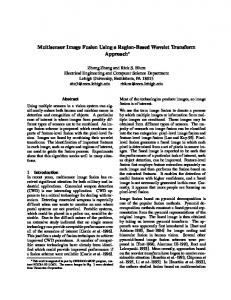
A particular focus was investigating separability of plantations from natural forest, as these A particular focus was investigating separability of plantations from natural forest, as these tend tend to be the most easily confused classes based on spectral information. Training and independent to be the most easily confused classes based on spectral information. Training and independent validation polygons were developed using multiple high resolution (HR) and field data sources. validation polygons were developed using multiple high resolution (HR) and field data sources. The The first HR data were collected over Kalimantan across 15 sites covering nearly ~65,000 ha in a first HR data were collected over Kalimantan across 15 sites covering nearly ~65,000 ha in a stratified stratified approach. Very high resolution airborne data covering the visible spectrum (R:G:B) at 50 cm approach. Very high resolution airborne data covering the visible spectrum (R:G:B) at 50 cm spatial spatial resolution were collected in November (26 November 2014). used to help resolution were collected in November (26 November 2014). These dataThese were data used were to help interpret interpret imagery and generate polygons. Figure 3 illustrates very high resolution airborne data over imagery and generate polygons. Figure 3 illustrates very high resolution airborne data over areas of areas of oil palm, forest, and highlights their structural characteristics (e.g.,spaces, planting spaces, oil palm, naturalnatural forest, and highlights their structural characteristics (e.g., planting natural natural forest canopy variation). forest canopy variation).
Figure Examplesfrom fromairborne airborneimagery imagery used used to to help forfor training Figure 3. 3. Examples help guide guidedevelopment developmentofofpolygons polygons training and validation. (A) shows oil palm plantation (top) and natural forest (bottom); (B) shows oil palm and validation. (A) shows oil palm plantation (top) and natural forest (bottom); (B) shows oil palm plantation (bottom right) and natural forest (top) highlighting natural forest canopy variability; plantation (bottom right) and natural forest (top) highlighting natural forest canopy variability; shows palmstand standwith withstructured structured planting planting and (C)(C) shows oiloilpalm and cleared cleared ground; ground;(D) (D)shows showsrepresentative representative natural forest canopy. natural forest canopy.
The second data source used for interpretation was a limited set of geofield photos. In an effort The second data source for interpretation was a limited geofield photos. In an to promote transparency andused improved land cover validation our teamset hasofbeen growing an online effort to promote transparency and improved land cover validation our team has been growing archive of field-level photos collected using a GPS-enabled camera (“geofield photos”). All geofield anphotos onlineare archive collected a GPS-enabled camera (“geofield linkedoftofield-level shape files photos or keyhole markupusing language (KML) files to store, display, andphotos”). share Allphotos. geofield photos are linked shape with files attributes or keyhole language files to store, KML files use a tag basedtostructure thatmarkup allow display. These (KML) photos are available display, and share photos. KML files a tag based structure with attributes that allow for viewing and sharing in Google Earthuse or any GIS platform at www.eomf.ou.edu/photos [36]. Atdisplay. this website, users search and a library of globalingeoreferenced photos product at These photos arecan available for share viewing and sharing Google Earthfield or any GISforplatform
Remote Sens. 2016, 8, 236
7 of 21
Remote Sens. 2016, 8, 236 of 21 www.eomf.ou.edu/photos [36]. At this website, users can search and share a library 77of global Remote Sens. 2016, 8, 236 of 21 georeferenced field photos for product development and validation. Figure 4 shows a representative development and validation. Figure 4 shows a representative geofield photo for creating an development validation. Figure 4 shows a representative geofield for creating geofield photo forand creating an agricultural training site. All photos forphoto the study regionsanwere agricultural training site. All photos for the study regions were considered for help interpreting agricultural training site. All imagery photos for the study regions were considered for help interpreting considered for help interpreting (Figure 5) and generating polygons. imagery (Figure 5) and generating polygons.
imagery (Figure 5) and generating polygons.
Figure 4. Geofield photo (A) riceagricultural agricultural site near West Kalimantan (B). (B). Figure 4. Geofield photo (A) ofof rice nearSingkawang, Singkawang, West Kalimantan Figure 4. Geofield photo (A) of rice agricultural site site near Singkawang, West Kalimantan (B).
Figure 5. Co-located examples of (A) airborne imagery; (B) Sentinel-1 (R:VV,G:VH,B:VH2);
Figure 5. Co-located examples 2 of (A) airborne imagery; (B) Sentinel-1 (R:VV,G:VH,B:VH ); 2 Figure Co-located examples of (A)(D) airborne imagery; (B) Sentinel-1 (R:VV,G:VH,B:VH ); ); and Landsat-8 (R:5, G:4, B:3). (C)5. PALSAR-2 (R:HH,G:HV,B:HV 2); and (D) Landsat-8 (R:5, G:4, B:3). (C) PALSAR-2 (R:HH,G:HV,B:HV (C) PALSAR-2 (R:HH,G:HV,B:HV2 ); and (D) Landsat-8 (R:5, G:4, B:3). 2
Remote Sens. 2016, 8, 236
8 of 21
We combined the high resolution imagery and field data with high resolution Google Earth Pro imagery to make final polygons. Google Earth Pro contains time series high resolution data that enables some temporal tracking of landscapes respective of the available dates. A total of 509 polygons containing 1,771,563 30 m pixels were carefully digitized across both study regions (Table 1). A range of plantation ages and landscape conditions (i.e., patch size, slope, interjuxtaposition, distance to urban areas) were included to build a robust calibration and validation data set. Plantation stand age was characterized into three broad classes (young, mixed, mature) based on visual interpretation and examining time-series high resolution imagery in Google Earth Pro. Table 1. Training data characteristics across both study regions. Class
# of Polygons
# of Pixels
Min Patch (ha)
Max Patch
Average Patch
Agriculture Developed Forest Plantation Water
87 94 100 134 94
32,992 37,262 1,103,423 282,215 315,671
0.5 0.4 0.8 4.0 1.3
636 557 1211 3865 11,370
33 35 1102 192 420
A suite of derivative indices was generated from both the SAR and optical data. These included common ratios (HH/HV2 ) and vegetation indices (NDVI, LSWI, SATVI, and NDTI) that have been found useful in other agroforest mapping studies, i.e., [18,19,32,33,35,37]. Texture indices were also generated in an effort to capture the “uniformity” or homogeneity of plantation canopy, spacing, and structure relative to natural forests. Several studies have found the integration of texture indices useful for mapping forest biometrics, i.e., [37]. Texture indices (Equations (5)–(12)) keyed off gray-level co-occurrence matrix (GLCM) included mean, variance, homogeneity, contrast, dissimilarity, entropy, second moment, and correlation [38]. Next, image statistics for the radar and optical variables were extracted to form a large database for mining, exploration, and model training. Sum Average pmeanq “
ÿ 2Ng ´ i “2
Variance psum of squares varianceq “
¯ ippx`yq piq ,
ÿ ÿ i
j pi ´ uq
(5) 2
ppi, jq,
˜ Homogeneity pinverse difference moment equationq “ Contrast “
ÿ Ng ´1
2 n“0 n
1
ÿ ÿ i
j
1 ` pi ´ jq2
!ÿ N ÿ N g g i “1
) ppi, jq , j “1
|i ´ j| “ n ) ÿ Ng ´1 !ÿ Ng ÿ Ng 2 Dissimilarity “ n ppi, jq , n “1 i “1 j “1 |i ´ j| “ n ÿ ÿ ` ˘ Entropy “ ´ i j ppi, jqlog ppi, jq , ÿ ÿ 2 Second Moment “ i j tppi, jqu , ř ř i j pi, jqppi, jq ´ u x uy Correlation “ σx σy
(6) ¸ ppi, jq,
(7) (8)
(9)
(10) (11) (12)
p(i,j) is the (I,j)th entry in a normalized gray-tone spatial-dependence matrix; Ng = Number of distinct gray levels in the quantized image; µx, µy are the means of px and py; σx, σy are the standard deviations of px and py. In this study, a classification and regression tree framework was carried out using the multiscale SAR and optical data (Figure 2). The ensemble, machine-learning, random forest algorithm [39]
Remote Sens. 2016, 8, 236
9 of 21
was employed to classify the remote sensing inputs for mapping plantation extent. A random forest is generated through the creation of a series of Classification and Regression Trees (CARTs) using bootstrapping, or resampling with replacement. Random forest is a flexible and powerful nonparametric technique that many mapping applications have recently implemented for a range of studies including mapping crops [40–42], wetlands [43–45], canopy height [46], algal blooms [47], urban sprawl [48], biomass [49], and many other thematic areas. For random forests as applied here, a number of decision trees were built and each time a split in a tree is considered, a random sample of m (m