remote sensing Article
Evaluation of Green-LiDAR Data for Mapping Extent, Density and Height of Aquatic Reed Beds at Lake Chiemsee, Bavaria—Germany Nicolás Corti Meneses *, Simon Baier, Juergen Geist
ID
and Thomas Schneider
ID
Aquatic Systems Biology Unit, Limnological Research Station Iffeldorf, Department of Ecology and Ecosystem Management, Technical University of Munich, Hofmark 1-3, 82393 Iffeldorf, Germany;
[email protected] (S.B.);
[email protected] (J.G.);
[email protected] (T.S.) * Correspondence:
[email protected]; Tel.: +49-(0)8856-810-50 Received: 25 October 2017; Accepted: 9 December 2017; Published: 13 December 2017
Abstract: Aquatic reed is an important indicator for the ecological assessment of freshwater lakes. Monitoring is essential to document its expansion or deterioration and decline. The applicability of Green-LiDAR data for the status assessment of aquatic reed beds of Bavarian freshwater lakes was investigated. The study focused on mapping diagnostic structural parameters of aquatic reed beds by exploring 3D data provided by the Green-LiDAR system. Field observations were conducted over 14 different areas of interest along 152 cross-sections. The data indicated the morphologic and phenologic traits of aquatic reed, which were used for validation purposes. For the automatic classification of aquatic reed bed spatial extent, density and height, a rule-based algorithm was developed. LiDAR data allowed for the delimitating of the aquatic reed frontline, as well as shoreline, and therefore an accurate quantification of extents (Hausdorff distance = 5.74 m and RMSE of cross-sections length 0.69 m). The overall accuracy measured for aquatic reed bed density compared to the simultaneously recorded aerial imagery was 96% with a Kappa coefficient of 0.91 and 72% (Kappa = 0.5) compared to field measurements. Digital Surface Models (DSM), calculated from point clouds, similarly showed a high level of agreement in derived heights of flat surfaces (RMSE = 0.1 m) and showed an adequate agreement of aquatic reed heights with evenly distributed errors (RMSE = 0.8 m). Compared to field measurements, aerial laser scanning delivered valuable information with no disturbance of the habitat. Analysing data with our classification procedure improved the efficiency, reproducibility, and accuracy of the quantification and monitoring of aquatic reed beds. Keywords: LiDAR; ALS; Phragmites australis; aquatic reed; OPALS; point cloud; classification; vegetation mapping
1. Introduction Reed beds provide important structural elements of lake ecosystems. Along a horizontal gradient that runs from the lake towards the bank, reed stocks are classified into three different ecological zones that occur either in water, transition, or in land zones [1]. The water reed at the expansion front of a reed stock is considered the most sensitive zone of a reed bed [2]. According to their definition, land reed beds are located in areas above water level, comprising an onshore/shoreward stock of multiple species, and usually growing in meadows [2]. Aquatic reed beds grow in locations that were flooded throughout the year. Lakewards stocks are pure stands of Phragmites australis, and are characterized by their low stem density (stems/m2 ) and longer sparse fertility [2]. Stocks of this macrophyte act as a buffer between land and water. They provide a key habitat for several endangered species [1], they physically protect banks from erosion, and they provide a food resource for various arthropods, Remote Sens. 2017, 9, 1308; doi:10.3390/rs9121308
www.mdpi.com/journal/remotesensing
Remote Sens. 2017, 9, 1308
2 of 17
birds, and mammals [3]. Aquatic reed beds are threatened, mainly due to mechanical, hydrological, anthropogenic, biological, and climatic causes [3–9]. Global warming influences, such as an increase in water temperature, extreme drought, and heavy rain events could additionally affect the growth and status of aquatic reed populations of freshwater lakes [10,11]. Changes in the abundance and density of reed beds can be quantified through the implementation of field measurements and remote sensing methodologies. Although on-site evaluations deliver highly accurate results, they are associated with high personnel, time, and financial expenses, as well as ecological disturbance of protected habitats [12]. Visual interpretation of multispectral aerial imagery has been the standard method to bypass this problem [7,13–15]. In the same way, analysis of satellite imagery has also been implemented [16–19]. These methodologies have contributed to the global monitoring of reed beds in wetlands and large lakes, where tens of hectares are covered by this type of vegetation. In the monitoring of small lakes with a limited presence of aquatic reed beds, spatial resolutions provided by satellite constellations are still too coarse for identifying stocks that are sparsely distributed or only comprise single reed individuals. This difficulty poses a serious limitation to monitoring spatial occurrence. The accurate identification of aquatic reed beds by analysis of optical imagery is affected by sun illumination, plant phenology, and spatial resolution. The position of the leaves’ and the stems’ incidence angle towards the sun causes differences in the spectral response and therefore, causes variances in the extent of quantification of sparse aquatic reed beds [7]. The imagery of official surveys is recorded normally for updating cadaster data and topographic maps, and not usually in the growth season (i.e., August to mid-September) when aquatic reed beds have their peak growth and maximum vitality. Accurate assessment is additionally hindered by shades, light reflection on the water surface, or vegetation reflectance. Although spatial resolution is sufficient for other purposes, sparse aquatic reeds cannot be identified in imagery with spatial resolutions lower than 20 cm per pixel [20,21]. Technological advancements in remote sensing science offer new possibilities in the characterisation of reed beds based on 3D data analysis. Very high spatial resolution multispectral imagery recorded with unmanned aerial vehicles and close range aerial photogrammetry have already supported the accurate mapping of land and aquatic reed beds [22]. In the same way, the biomass of wetland Phragmites australis [23], of wetland vegetation mapping [24–26], and characterisation of the land reed bed habitat quality [27] have all been achieved by applying Light Detection and Ranging (LiDAR) technologies alone or in combination with other data types (e.g., hyperspectral data). Nevertheless, the level of agreement at which height of, extent of, and density of aquatic reed beds can be mapped with LiDAR data remains unknown. The new LiDAR system configured to function in the green wavelength of the electromagnetic spectrum offers new possibilities in the research of aquatic reed beds. Green light, the opposite of infrared, propagates in water by reflecting off the bottom surface, or in medium content materials [28]. In addition, green light not only propagates in water but can also reflect off land surfaces. These characteristics make the Green-LiDAR scanner suitable in mapping bathymetry [29], bottom structures [30,31], or even for topo-bathymetric applications [32,33]. Extents are important in the monitoring of aquatic reed beds, in which the mapping of the shoreline and the frontline are crucial. The technological benefits of a Green-LiDAR scanner could contribute to the accurate mapping of red bed boundaries. The frontline is scanned from reed stems and leaves above the water surface and thanks to green light propagation, the shoreline can be obtained independent of the water surface level during surveying. Aquatic reed is an important indicator for the ecological assessment of freshwater lakes listed by the European Water Framework Directive (EU-WFD). As in other European countries, German federal state environmental agencies have to regularly report on the ecological status of freshwater lakes which involves a substantial monitoring effort. The core objective of the present study was to evaluate the applicability of Green-LiDAR technology in aquatic reed monitoring. We addressed the following research questions by focusing on the accuracy of diagnostic determination:
Remote Sens. 2017, 9, 1308
3 of 17
evaluate the applicability of Green-LiDAR technology in aquatic reed monitoring. We addressed the 3 of 17 by focusing on the accuracy of diagnostic determination:
Remote Sens. 2017, 9, 1308 following research questions
• •• ••
How accurate is the estimation of aquatic reed extent in LiDAR point clouds? How accurate accurate is is the the estimation estimation of of aquatic aquatic reed reed extent densityininLiDAR LiDARpoint pointclouds? clouds? How How accurate accurately aquatic reed DSMs bedensity calculated from LiDAR point clouds? How is can the estimation of bed aquatic reed in LiDAR point clouds?
• How accurately can aquatic reed bed DSMs be calculated from LiDAR point clouds? 2. Material and Methods 2. Material and Methods 2.1. Study Area 2.1. Study Area The Chiemsee is the largest lake in Bavaria (80 km2) with a maximum depth of 73 m and a 3 volume 2048 hmis [34]. It is located km southeast of depth Munich at m anand approximate Theof Chiemsee the largest lake inapproximately Bavaria (80 km280 ) with a maximum of 73 a volume altitude of 3518 m It above sea level (m.a.s.l.). During last five the extent of the reed of 2048 hm [34]. is located approximately 80 km the southeast ofdecades, Munich at anspatial approximate altitude of population by about 50%the at the [2].the Substantial reed of beds thepopulation Chiemsee has are 518 m abovehas seadeclined level (m.a.s.l.). During lastChiemsee five decades, spatial extent the at reed still existent and their has been well documented this lake wasexistent selectedand for declined by about 50%decrease at the Chiemsee [2]. Substantial reed which beds atwas the why Chiemsee are still our study. On the northwest side of the Chiemsee and at the Herreninsel, the most representative their decrease has been well documented which was why this lake was selected for our study. On the stocks of aquatic reed are stilland present Throughthe anmost analysis of previous surveyed data, northwest side of the Chiemsee at the[21]. Herreninsel, representative stocks of aquatic reedfield are observations, distribution stocks, andofof water depth, thedata, areasfield of interest (AOI)distribution were selected for still present [21]. Through an analysis previous surveyed observations, stocks, gathering validation data. The actual density of reed stems obtained from field observation was also and of water depth, the areas of interest (AOI) were selected for gathering validation data. The actual considered. A total of from 14 AOIs the occurrence Phragmites A australis at a mean of density of reed stemsnumber obtained fieldwith observation was alsoofconsidered. total number of 14area AOIs 2 (100 m in length at varying width) were selected for this 2 1694 m study. AOIs were delimited at with the occurrence of Phragmites australis at a mean area of 1694 m (100 m in length at varying width) Aiterbacher at the shores of Holzen (AOI-2,) atWinkel Keilbacher Eck at (AOI-3), in Kailbacher were selectedWinkel for this(AOI-1), study. AOIs were delimited at Aiterbacher (AOI-1), the shores of Holzen Winkel (AOI-4 and -5), Scheren (AOI-6), atWinkel the shores town (AOI-7 andat-8), at (AOI-2,) at Keilbacher Eckat (AOI-3), in Kailbacher (AOI-4ofand -5), Mühln at Scheren (AOI-6), the and shores Herreninsel (AOI-9, -10, -11, -12, -13, -14). In order to consider the variability of vegetation status, of town Mühln (AOI-7 and -8), and at Herreninsel (AOI-9, -10, -11, -12, -13, -14). In order to consider the AOIs wereofselected in areas ofAOIs different of protection: (a) protected long, (b) variability vegetation status, werelevels selected in areas of different levelsall of year protection: (a) protected protected only during breeding season,the andavian (c) inbreeding areas without any form of areas environmental protection all year long,the (b)avian protected only during season, and (c) in without any form of (Figure 1). environmental protection (Figure 1).
Figure 1. Location of the study area at country (a) and local level (b). Distribution of Areas of Interest (AOIs) at the Chiemsee. Coordinate System is Deutsches Hauptdreiecksnetz (DHDN) Gauss Krüger Zone 4 (European Petroleum Survey Group (EPSG) 31468).
Remote Sens. 2017, 9, 1308
4 of 17
Figure 1. Location of the study area at country (a) and local level (b). Distribution of Areas of Interest at the Chiemsee. Coordinate System is Deutsches Hauptdreiecksnetz (DHDN) Gauss Krüger4 of 17 Remote(AOIs) Sens. 2017, 9, 1308 Zone 4 (European Petroleum Survey Group (EPSG) 31468).
2.2. Airborne Airborne Laser Laser Scanning Scanning Processing Processing Chain Chain 2.2. The analysis analysis and and classification of Airborne The classification of Airborne Laser Laser Scanning Scanning (ALS) (ALS) datasets datasets was was performed performed with with the modular program system OPALS 2.2.0.0 [35]. The software provides modules for aa complete the modular program system OPALS 2.2.0.0 [35]. The software provides modules for complete processing ALS data. data. Pre-processed Pre-processed LiDAR LiDAR point point clouds clouds were were imported imported into into the the OPALS OPALS data data processing chain chain of of ALS manager and the quality was assessed according to strip adjustment and outliers (noise). According manager and the quality was assessed according to strip adjustment and outliers (noise). According to the the information obtained from from the the quality quality control, control, no no further further calibration calibration (e.g., (e.g., strip strip adjustment, adjustment, to information obtained geometry calibration) calibration) was was needed. Point cloud cloud classification classification was was then then performed, performed, and and raster raster and and geometry needed. Point vector file results were compared to field data and aerial imagery (Figure 2). vector file results were compared to field data and aerial imagery (Figure 2).
Figure 2. Airborne Laser Scanning (ALS) processing and decision chain applied for modelling aquatic Figure 2. Airborne Laser Scanning (ALS) processing and decision chain applied for modelling aquatic reed beds. reed beds.
The topo-bathymetric data collection took place on 21 September 2015, between 15h00 and 16h30 The topo-bathymetric collection took on 21 September 2015,VQ-880G between(Riegl 15h00LMS, and (UTC) during sunny weatherdata conditions using theplace hydrographic laser scanner 16h30 duringThis sunny weather using the hydrographic scanner VQ-880G Horn, (UTC) Österreich). device is aconditions progressive palmer scanner withlaser a laser beam in the (Riegl green LMS, Horn, Österreich). This device is a progressive palmer scanner with a laser beam in set the to green wavelength (532 nm) of the electromagnetic spectrum. The laser pulse repetition rate was 550 wavelength (532 nm) of the electromagnetic spectrum. The laser pulse repetition rate was set to kHz and the laser beam divergence was set to 1 mrad. The mission was executed at an altitude of 550 kHz and the laser beam divergence was set to 1 mrad. The mission was executed at an altitude of approximately 400 m above ground. The scan width was about 400 m and the footprint was 40 cm approximately 400 m above ground. The scan width was about 400 m and the footprint was 40 cm (diameter). A total of 58 strips was collected for the study area (29 back and forward scans). Point (diameter). total of 58with strips collected obtained for the study (29 back forwardSystem scans). (POS) Point clouds wereAregistered thewas information by aarea Position and and Orientation clouds were registered with the information obtained by a Position and Orientation System (POS) mounted on-board, and were improved by correction measurements sent by a Differential Global mounted on-board, and were improved byland. correction measurements a Differential Global Positioning System (DGPS) base station on Orientation data was sent also by recorded by the Inertial Positioning System (DGPS)during base station land.photographs Orientation data by the Inertial Measurement Unit (IMU) flight.on Aerial withwas a 0.1also m recorded spatial resolution were Measurement Unit (IMU) during flight. Aerial photographs with a 0.1 m spatial resolution were additionally recorded during the same flight for validation purposes. additionally recorded during same flight purposes. Data pre-processing wastheexecuted by for thevalidation data provider (AHM Airborne Hydro Mapping Data pre-processing was executed by the data provider (AHM Hydro Mapping GmbH) GmbH) using the software RiProcess. Strip adjustment was the firstAirborne step in the pre-processing chain. using the software RiProcess. Strip adjustment was the first step in the pre-processing The acquired accuracy was 10 cm (Standard Deviation). Secondly, based on the laser data,chain. well The acquired accuracy was 10 cm (Standard Deviation). Secondly, based on the laser data, well distributed Ground Control Points (GCP) from roof corners and streets lane markers were defined distributed Ground Control from roof corners and streets lane markers were defined across the study area. The 48Points GCPs(GCP) were measured by the research team with a tachymeter Leica across the study area. The 48 GCPs were measured by the research team with a tachymeter Leica TCRP 1201 R300 for fine registration. Absolute registration achieved an accuracy of 8 cm, and the TCRP 1201 R300 Absolute registration achieved an accuracy of 8 outliers). cm, and the point 2 (which point density of for thefine rawregistration. data was approximately 200 points/m included Finally, 2 (which included outliers). Finally, outliers density of the raw data was approximately 200 points/m outliers were filtered and the point clouds from the specific AOIs were exported in Log ASCII were filtered and1.4 theformat. point clouds from the specific AOIs were exported in Log ASCII Standard (LAS) Standard (LAS) 1.4 format.
Remote Sens. 2017, 9, 1308
5 of 17
Quality control was performed before processing the ALS data sets. Point clouds were firstly, visually inspected. Attributes stored in the OPALS Data Manager (ODM) were examined in a 3D environment (opalsView) to identify potential errors in the already pre-processed product. Special attention was paid to the point geometry and the outlier filtering in water-land transition areas. An absence of points from water surfaces was identified in shallow water areas. Planar water surfaces cause specular reflections and therefore surface echo dropouts [32]. The overall low amount of noise in the point clouds delivered from the provider revealed that additional filtering was not needed. The package opalsQuality was then used for the quantification of point cloud quality. Cloud density and strip differences were analysed by means of density maps and statistical measurement. Since light propagates differently in water than in air, the points under the water surface appeared to have shifted and therefore had to be corrected. The module implemented for the refraction correction was opalsSnellius [28]. This correction was computed with the refractive index, coordinates of origin, incidence angle, and specification of the water lever. First, to calculate the refractive index, the sine of the angle of incidence was divided by the sine of the angle of refraction [36]. Refractive index varies depending on properties of transmission media (e.g., temperature, pH) and wavelength of incoming radiation. For variable temperature and salinity conditions, and for a green laser (532 nm wavelength), the refractive index is n = 1.33538 [36]. Second, the coordinates of the laser origin and the incidence angle were obtained from the trajectory information recorded by IMU and POS. Third, the Air–Water Interface (AWI) was modelled in Quantum Geographic Information System (QGIS) by creating a raster in which all pixels values corresponded to the height of the water surface according to the daily measurements of the master data gauge at Stock, Chiemsee [37]. The water level used (517.93 m.a.s.l.) for the water surface modelling was the measurement taken when the scanning flight took place. The laser penetration depth in the water body was about 10 m, which was approximately 8 m after correcting for light refraction. 2.2.1. Classification of Green-LiDAR Data Statistical parameters for LiDAR point clouds were calculated for describing point attributes with the module opalsPointStats. OPALS calculates statistical features by first selecting points and then relating them to a reference model. The selection of points was based on an infinite vertical cylinder (searchMode = d2); the reference model was a “horizontalPlane”. Since the laser footprint at ground level was around 0.4 m in diameter, the cylinder radius (searchRadius) was set to 0.2 m for the majority of calculations. In the model “horizontalPlane”, the samples were reduced in relation to a plane passing through the feature point. Calculated statistics for identifying patterns in point clouds were ranked (rank) and point density (pdens). Rank statistic was calculated as the relative position (0 = local minimum and 100 = local maximum) of the feature point within its vertical neighbourhood. The feature pdens is the number of points in relation to the area/volume of the search cylinder. Since the usual measurement units for point density is points/m2 , a cylinder searchMode with a searchRadius of 0.5 m was selected as the most proximate value to a square meter (Figure 3). Filtering was crucial for the classification, since it allowed for points to be defined when a new attribute had to be calculated (processing filtering) in relation to the local neighbourhood (neighbourhood filtering). The classification was performed with the module opalsAddInfo. In order to define the threshold values, point clouds were inspected through cross-sections every metre with the module opalsSection. Special attention was placed on spatial distribution, density, and intensity of points. Cross-sections revealed that height and vertical distribution of points are important factors to differentiate dense and sparse reed beds.
Remote Sens. 2017, 9, 1308
6 of 17
Remote Sens. 2017, 9, 1308
6 of 17
Figure 3. Graphical representation of methods and statistics used for classifying aquatic reeds in point Figure 3. Graphical representation of methods and statistics used for classifying aquatic reeds in point clouds obtained from Green-Light Detection and Ranging (LiDAR). clouds obtained from Green-Light Detection and Ranging (LiDAR).
2.2.2. Validation Data 2.2.2. Validation Data Field data were collected by means of cross-sections and square sample plots. The measurements Field data were collected by means of cross-sections and square sample plots. The measurements started by defining a one hundred-metre line parallel to the shore. A measuring tape was placed started by defining a one hundred-metre line parallel to the shore. A measuring tape was placed perpendicularly to this line every ten metres. Measurement started from the waterside and finished perpendicularly to this line every ten metres. Measurement started from the waterside and finished on the shoreline (i.e., the point at which water and land have the same height). At every metre along on the shoreline (i.e., the point at which water and land have the same height). At every metre along the cross-sections, water depth and reed stem height were measured to the nearest centimetre and the cross-sections, water depth and reed stem height were measured to the nearest centimetre and decimetre, respectively. The frontline was then surveyed as the location in the cross-section where decimetre, respectively. The frontline was then surveyed as the location in the cross-section where the the first reed stem occurs. Plotting the coordinates of shorelines and frontlines in every cross-section first reed stem occurs. Plotting the coordinates of shorelines and frontlines in every cross-section in in QGIS allowed the aquatic reed extents to be calculated. Based on expert knowledge, one or two QGIS allowed the aquatic reed extents to be calculated. Based on expert knowledge, one or two square square sample plots of 1 square metre each were placed where differences in stem density were sample plots of 1 square metre each were placed where differences in stem density were identified. identified. The parameter’s density2 (stems/m2), stem diameter, number of stems with and without The parameter’s density (stems/m ), stem diameter, number of stems with and without shoots, and shoots, and the number of green and dried (brown) stems were additionally recorded (Figure 4). Data the number of green and dried (brown) stems were additionally recorded (Figure 4). Data collected collected from the square sample plots were used to verify the classification of point clouds. In from the square sample plots were used to verify the classification of point clouds. In addition, addition, data from cross-sections (i.e., the height of reed stems) were used as independent data to data from cross-sections (i.e., the height of reed stems) were used as independent data to validate validate the derived Digital Surface Models (DSM). Trimble Geo XT was the DGPS system the derived Digital Surface Models (DSM). Trimble Geo XT was the DGPS system implemented for implemented for measuring reference points. Post-processing was executed with the software measuring reference points. Post-processing was executed with the software Trimble GPS Pathfinder Trimble GPS Pathfinder Office. The base station SOPAC Wettzell Daily with L2 and the Global Office. The base station SOPAC Wettzell Daily with L2 and the Global Navigation Satellite System Navigation Satellite System (GLONASS) capability was selected for differential correction. The (GLONASS) capability was selected for differential correction. The coordinate reference system coordinate reference system implemented was the Deutsches Hauptdreiecksnetz (DHDN) Gauss– implemented was the Deutsches Hauptdreiecksnetz (DHDN) Gauss–Krüger Zone 4. Krüger Zone 4.
Remote Sens. 2017, 9, 1308 Remote Sens. 2017, 9, 1308
7 of 17 7 of 17
Figure Collection of of Reference Reference Points Points (RPs) as an an example example of of AOI-3. AOI-3. Background Background is is an an orthorectified orthorectified Figure 4. 4. Collection (RPs) as aerial aerial photograph photograph in in true true colour colour of of the the Landesamt Landesamt für für Digitalisierung, Digitalisierung, Breitband Breitband und und Vermessung Vermessung (LDBV), Differential Global Global Positioning Positioning System System (DGPS) (DGPS) Trimble Trimble GeoXT (LDBV), 2015 2015 (a). (a). Differential GeoXT and and an an antenna antenna Hurricane L1 used for georeferencing RPs (b). Aerial view of square transect measurements Hurricane L1 used for georeferencing RPs (b). Aerial view of square transect measurements along along aa cross-section (c). One-hundred metre line parallel to the shore with 10 m sections (d). cross-section (c). One-hundred metre line parallel to the shore with 10 m sections (d).
2.2.3. Assessment of Aquatic Reed Extents and Classification Classification Accuracy Accuracy Extents Extents of aquatic reed reed beds were were evaluated evaluated based based on on two criteria. criteria. First, the extents derived from LiDAR were compared withwith the ones obtained from from field measurements, by means LiDAR data datafor forevery everyAOI AOI were compared the ones obtained field measurements, by of correlation analysis.analysis. Since measured and derived surfaces surfaces can havecan the have samethe extents different means of correlation Since measured and derived samebut extents but shapes, correlation analysis ofanalysis the extents wasextents complemented by an assessment geometrical differentthe shapes, the correlation of the was complemented by an of assessment of similarity. As a second criterion, the separation distance of two geometrical objects (polygons) in a geometrical similarity. As a second criterion, the separation distance of two geometrical objects metric spaceinwas measured Distance Pairwise). The smaller the resulting value, more (polygons) a metric space(Hausdorff was measured (Hausdorff Distance Pairwise). The smaller the the resulting similar themore geometrical are [38]. shapes In addition and In to addition support this metric, this the Root Mean value, the similar shapes the geometrical are. [38]. and last to support last metric, Squared the lengths on the field in relation to the lengths the Root Error Mean(RMSE) SquaredofError (RMSE)of ofcross-sections the lengths of measured cross-sections measured on the field in relation obtained from obtained LiDAR data was assessed. to the lengths from LiDAR data was assessed. The assessment assessment of of classification classificationaccuracy accuracywas was achieved a confusion or error matrix. achieved by by a confusion or error matrix. The The classification result compared withindependent independentvalidation validationdata. data. Two Two approaches approaches were classification result waswas compared with implemented for the accuracy assessment of aquatic reed classification. classification. First, the classification was compared compared with with on-field on-field collected collected data. data. A total of 249 square square sample sample plots plots of of 11 m m22 each were collected on-field on-field and and used used for validation, validation, out out of which 127 and 152 were measured in dense and sparse aquatic reed imagery with a resolution of 0.1 collected at theatsame time reed beds, beds,respectively. respectively.Second, Second,RGB RGB imagery with a resolution of m/pxl, 0.1 m/pxl, collected the same as theas ALS took place, used forused visual validation. Samples were collected time thesurvey ALS survey took was place, was forinterpretative visual interpretative validation. Samples were randomly and stratified (i.e., classes). Since theSince mapthe hasmap less has thanless 12 than classes theand study is collected randomly and stratified (i.e., classes). 12 and classes thearea study 2), a minimum less 1 million acres (4046.9 km2 ), akm minimum of 50 points shouldshould be collected for every areathan is less than 1 million acres (4046.9 of 50 points be collected for single every class A[39]. totalA oftotal 150 points and proportionally distributed (Table 1)(Table across 1) theacross total single[39]. class of 150 were pointsgenerated were generated and proportionally distributed extent of extent each class. the total of each class.
Remote Sens. 2017, 9, 1308
8 of 17
Table 1. Sample distribution according to extent of classes. Class
Area (m2 )
Area (ha)
Number of Samples
Sparse Aquatic Reed Dense Aquatic Reed
4843 9037
0.4843 0.9037
50 100
The error matrix shows a percentage of pixels from each class labelled correctly as well as the proportions of pixels erroneously labelled into a different class [40]. These percentages are expressed as the overall accuracy (OA), producer´s accuracy (PA) and user´s accuracy (UA). Additionally, the chance of agreement was also calculated with the Kappa coefficient [41]. 2.2.4. Accuracy Assessment of DSM Two assessments were accomplished in order to validate the accuracy of estimated DSM. First, the height of a flat surface (i.e., quay, dock) in DSM was compared to the respective one acquired with an onsite survey. Second, the derived aquatic reed heights were assessed on their elevation values in comparison with those measured at each AOI. Distribution type of the height residuals was calculated with the sample skewness and its significance. For a normal distribution, the Mean Error (ME), Standard Deviation (SD), and the Root Mean Square Error (RMSE) were obtained for evaluating the closeness agreement between the observed and the modelled height of reeds (Table 2). The rasterisation of the point clouds was performed using a moving (tilted) plane interpolator (movingPlanes) in OPALS software. Detailed information about this interpolator can be found in [35]. Table 2. Accuracy measures for Digital Evidence Management system (DEms) presenting normal distribution of residuals. µ=
Mean Error
1 n
s Standard Deviation Root Mean Square Error
σ=
1 (n−1)
RMSE =
n
∑ ∆hi
[42]
i=1 n
∑ (∆hi − µ) i=1 s 1 n
n
2 ∑ ∆hi
2
[42] [42,43]
i=1
n is the number of tested points in the sample (sample size) and ∆hi represents the difference between RP and Digital Service Models (DSMs) for a point i. The assessment of vertical accuracy was performed considering the Air–Water Interface (AWI) as the zero point. The relative stem height (RSH) was obtained by subtracting the absolute height (length from flower to sediment) minus the water depth. The same absolute height of the water surface used for modelling AWI was used for obtaining the RSH.
3. Results 3.1. Point Cloud Classification The classification was performed at point level and by means of a decision tree. Development of the rule-based algorithm was based on combining previous knowledge from fieldwork and visual inspections of AOIs point clouds. By means of statistical parameters for every point cloud, several classes were categorised in every point cloud (Figure 5). Dense and Sparse Aquatic Reed beds were classified in consideration of the statistical parameters of height and density. With the obtained classes, quantification of extents, as well as the expansion of frontline and shoreline was possible. The classification procedures were executed after quality control. The absolute registration accuracy was 8 cm and strip differences averaged 0.022 m, SD 0.039 m, and RMSE 0.045 m. Registration accuracy and low strip differences were accepted as suitable for the study objectives and no further calibration was performed.
Remote Sens. 2017, 9, 1308
9 of 17
Remote 9, 1308 9 of 17 and lowSens. strip2017, differences were accepted as suitable for the study objectives and no further calibration was performed.
Figure 5. Classification scheme used in OPALS for density classification of aquatic reed beds. Dashed Figure 5. Classification scheme used in OPALS for density classification of aquatic reed beds. Dashed line boxes are intermediate classes and coloured boxes represent final classes. Point statistics and line boxes are intermediate classes and coloured boxes represent final classes. Point statistics and attributes used for classification thresholds are described between classes. Detailed explanation of attributes used for classification thresholds are described between classes. Detailed explanation of statistics used can be found in Section 2.2.1. statistics used can be found in Section 2.2.1.
The structural characteristics obtained from cross-sections extracted in one-metre intervals The characteristics from cross-sections extracted inand one-metre intervals through all structural point clouds were equallyobtained important. Spatial distribution of points their height in through all point clouds were equally important. Spatial distribution of points and their height relation to the AWI were key factors for density classification. The height of sparse aquatic reed beds relation to the between AWI were key factors forAdensity Thetoheight sparse aquatic reed forinall AOIs varied 1.80 and 2.40 m. height classification. of 2 m was found be theofmost suitable value beds for all AOIs varied between 1.80 and 2.40 m. A height of 2 m was found to be the most suitable for an accurate automatic classification of all point clouds (Figure 6). The density of points was the value parameter for an accurate automatic classification of all point clouds 6). characterised The density of second considered for classification. Dense aquatic reed(Figure beds are bypoints tall was the second parameter considered for classification. Dense aquatic reed beds are characterised reeds with a height greater than 2 m (520 m.a.s.l.), a large number of leaves in the upper canopy level,by tallbare reeds withstems a height greater than 2 m (520 m.a.s.l.), a large number leaves in thewere upper canopy and thick in the lower canopy level. Regarding the LiDARofdata, points equally level, and in bare thickstocks stemsand in the lower canopy level. Regarding data, points were in equally distributed sparse accumulated in the upper canopy the for LiDAR dense stocks. This break the distributed in sparse stocks and accumulated in the upper canopy for dense stocks. This break in the spatial distribution was easily identifiable in the points between the AWI and the 1.5 m relative height spatial distribution identifiable in the points AWIthis andheight, the 1.5 m height (519.5 m.a.s.l.). Oncewas the easily density was calculated for allbetween values the under therelative maximum (519.5 m.a.s.l.). Once the was calculated forclassification all values under this height, the maximum frequent value in every AOIdensity was always selected for thresholds. For clouds with 2–3frequent strips, value in every AOI was always selected for classification thresholds. For clouds with 2–3 strips, this this threshold value was 80 points/m2. According to this definition, Sparse Aquatic Reed beds were 2 threshold was 80 points/m . According to thiswere definition, Aquatic Reed beds were classified andvalue the remaining points without classification assignedSparse to Dense Aquatic Reed beds. classified and the remaining points without classification were assigned to Dense Aquatic Reed beds.
Remote Sens. 2017, 9, 1308
10 of 17
Remote Sens. 2017, 9, 1308
10 of 17
Figure 6. Classification of Sparse Aquatic Reed beds according to stem height below 2 m (rank), Figure 6. Classification of Sparse Aquatic Reed beds according to stem height below 2 m (rank), density density of points under a height of 1.50 m (pdens), and in combination with processing and of points under a height of 1.50 m (pdens), and in combination with processing and neighbourhood neighbourhood filtering. Grey colours represent to unclassified points, and black and red to areas of filtering. Grey colours represent to unclassified points, and black and red to areas of sparse and dense sparse and dense aquatic reeds, respectively. aquatic reeds, respectively.
3.2. Assessment of Aquatic Reed Bed Extents 3.2. Assessment of Aquatic Reed Bed Extents The result of the classification showed that a total of 1.388 hectares (100%) were aquatic reed The result of the classification showed that a total of 1.388 hectares (100%) were aquatic reed beds. beds. More than half of the reed beds were identified as Sparse Aquatic Reed (65%—0.9037 ha) and More than half of the reed beds were identified as Sparse Aquatic Reed (65%—0.9037 ha) and the the remaining 35% were identified as Dense Aquatic Reed (0.4843 ha). The correlation analysis remaining 35% were identified as Dense Aquatic Reed (0.4843 ha). The correlation2 analysis between between onsite and LiDAR derived extents showed a highly positive correlation (R = 0.75). However, similar extents do not mean similar border shapes and therefore correlation was complemented by a symmetrical assessment of polygon shapes and cross-section lengths (Figure 7). The methodology
Remote Sens. 2017, 9, 1308
11 of 17
onsite and LiDAR derived extents showed a highly positive correlation (R2 = 0.75). However, similar extents do not mean similar border shapes and therefore correlation was complemented by a symmetrical Remote Sens. 2017, 9, 1308 11 of 17 assessment of polygon shapes and cross-section lengths (Figure 7). The methodology implemented for the aquatic reed front and shoreline delimitation showed a high similarity with the derived LiDAR implemented for the aquatic reed front and shoreline delimitation showed a high similarity with the resultsderived from the AOIs, especially in parallel frontlinesinand shorelines (e.g., AOI-1). Hausdorff distances LiDAR results from the AOIs, especially parallel frontlines and shorelines (e.g., AOI-1). ranged from 5.74 m (AOI-1) 12.69 obtained from the analysis Hausdorff distances rangedtofrom 5.74mm(AOI-8). (AOI-1) toSimilar 12.69 m results (AOI-8).were Similar results were obtained from of cross-sections lengths. The RMSE values from 0.69 m (AOI-1) m (AOI-8). the analysis of cross-sections lengths. Theranged RMSE values ranged from 0.69to m 4.86 (AOI-1) to 4.86 m (AOI-8).
Figure 7. of Examples of shape similarity onsite (grey and derived from LiDAR data outline). Figure 7. Examples shape similarity measuredmeasured onsite (grey fill) andfill) derived from LiDAR data (black (black outline).
3.3. Assessment of Aquatic Reed Bed Densities
3.3. Assessment of Aquatic Reed Bed Densities
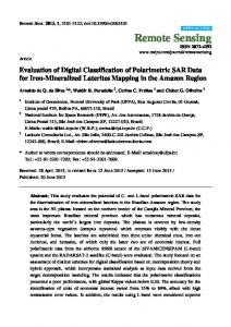
The first of the vegetation density map revealed (OA)of of72.7% 72.7% for The assessment first assessment of the vegetation density map revealedan anoverall overall accuracy accuracy (OA) the validation compared to field data.data. TheThe reference points usedfor forthis this assessment obtained for the validation compared to field reference points(RP) (RP) used assessment obtained a 0.46am horizontal andand 0.540.54 m vertical precision correction. The mean Horizontal 0.46 m horizontal m vertical precisionafter after differential differential correction. The mean Horizontal and Vertical Dilution of Precision whichall allthe the measurements measurements (RPs) took place waswas 1.3 and 2.1, 2.1, and Vertical Dilution of Precision at at which (RPs) took place 1.3 and respectively. A mean of 17 measurements was recorded for every RP. The Producer’s Accuracy (PA) respectively. A mean of 17 measurements was recorded for every RP. The Producer’s Accuracy (PA) showed that 85.6% of the sparse areas werecorrectly correctly identified, identified, but to to thethe User’s Accuracy showed that 85.6% of the sparse areas were butaccording according User’s Accuracy (UA) for the same class, this was true only 68.2% of the time (Table 3). Contrarily, 59.7% (PA) of dense (UA) for the same class, this was true only 68.2% of the time (Table 3). Contrarily, 59.7% (PA) of dense areas were identified as such, with 80.4% (UA) of the classification truly corresponding to that areas were identified as such, with 80.4% (UA) of the classification truly corresponding to that category. category. The Kappa coefficient for this assessment suggests that the observed classification is 50% The Kappa coefficient for this assessment suggests that the observed classification is 50% better than better than that which resulted by chance. that which resulted by chance. Table 3. Confusion matrix for classification assessed against field data (left) and aerial imagery (right).
Table 3. Confusion matrix for classification assessed against field data (left) and aerial imagery (right). Reference Data
User’s Classified Reference Data Dense Sparse Total Accuracy ClassifiedData User’s (%) Dense Sparse Total Data Accuracy (%) Dense 74 18 92 80.4 Dense 74 18 92 80.4 Sparse 50 1.07 157 68.2 Sparse Total 50 68.2 124 1.07 125 157 249 Total
124
Producer’s
Producer’s Accuracy (%) 59.7 Accuracy (%)
125
59.7
85.6
249
85.6
Overall Accuracy = 72.7; Kappa Overall Accuracy (%)(%) = 72.7; Kappa = 0.5= 0.5
Reference Data
Classified Data Classified Data
Dense Dense
Reference Data
Sparse
Sparse
Total
User’s Accuracy(%) User’s
Total
Accuracy(%)
Dense 47 3 50 94 Dense 47 3 50 Sparse 3 97 100 97 Sparse Total 503 10097 50 100 Total 50 100 50 Producer’s Accuracy 94 97 150 Producer’s 94 97 150 Accuracy (%) (%) Overall Accuracy (%) = 96; Overall Accuracy (%) = 96;Kappa Kappa==0.91 0.91
94 97
Remote Sens. 2017, 9, 1308 Remote Sens. 2017, 9, 1308
12 of 17 12 of 17
Results differed for the second accuracy assessment of classified density. Very Very high-resolution high-resolution aerial imagery (0.1 m/pxl) taken at the same time and during the same flight as the ALS was m/pxl) taken at the same time and during implemented for this task. An OA of 96% with the Kappa coefficient of 0.91 was obtained from the evaluation evaluation (Table (Table 3). 3). High classification classification accuracy accuracy was explained by the unbiased visual interpretative validation applied by the same operator (reed expert) and for all the AOIs represented on RGB RGB data. data. Both classes (Dense and Sparse) showed a high level of UA and PA, for which the values were 94% and 97% for sparse and dense classes, respectively. An area on the ground will actually be what the classification reveals 94% and 97% of the time. In the same way, the proximity to one of the values from the Kappa coefficient coefficient indicates indicates aa “true” “true” agreement agreement with withthe theclassification classification(Figure (Figure8). 8).
Figure 8. 8. Classification of dense dense and and sparse sparse aquatic aquatic reed reed (AOI-6). (AOI-6). Figure Classification of
3.4. Accuracy Assessment for for Calculated Calculated DSM DSM of of Aquatic Aquatic Reed Reed Beds Beds 3.4. Accuracy Assessment The moving moving tilted tilted plane plane interpolator interpolator (movingPlanes) (movingPlanes) in in combination combination with with aa defined defined number number of of The neighbours (16) allowed for the creation of raster files with a minimum grid size of 10 centimetres. neighbours (16) allowed for the creation of raster files with a minimum grid size of 10 centimetres. After evaluating evaluating observations observations against against modelled modelled height, height, an an accuracy accuracy assessment assessment for for flat flat structures structures After showed a total RMSE of 0.1 m, while for vegetation height, it showed a RMSE of 0.8 m. The showed a total RMSE of 0.1 m, while for vegetation height, it showed a RMSE of 0.8 m. The distribution distribution of the residuals in both assessments was not significantly skewed, since the skewness of the residuals in both assessments was not significantly skewed, since the skewness factors for all 14 √ factorswere for all 14 AOIs weretimes lower than two times standard error(SES of the = to 6⁄the n). AOIs lower than two the standard errorthe of the skewness = skewness 6/n). In (SES relation In relation to the vegetation height assessment, a perfect normal distribution resulted in residuals vegetation height assessment, a perfect normal distribution resulted in residuals from AOI-7 and -12. from AOI-7 and -12. Meanwhile, the asymmetries lowest and greatest asymmetries were in AOI-5and (skewness Meanwhile, the lowest and greatest found were in AOI-5found (skewness = 0.52) AOI-11 = 0.52) and AOI-11 (skewness = −0.47). Overall, 1279 independent observations were used to assess (skewness = −0.47). Overall, 1279 independent observations were used to assess the vertical accuracy thevegetation vertical accuracy of DSM. vegetation heights in analysis DSM. The correlation analysis and between the observed of heights in The correlation between the observed predicted relative 2 2 and predicted relative stem height (RSH) revealed a low positive correlation (R = 0.42). stem height (RSH) revealed a low positive correlation (R = 0.42). 4. Discussion This study suggests that ALS provides a highly accurate alternative to the currently applied field-based methodologies for aquatic reed bed monitoring. In contrast to classical monitoring, ALS
Remote Sens. 2017, 9, 1308
13 of 17
4. Discussion This study suggests that ALS provides a highly accurate alternative to the currently applied field-based methodologies for aquatic reed bed monitoring. In contrast to classical monitoring, ALS involves no direct entry of the habitat and no disturbance of the species living there, and therefore, only samples of the study area are needed for field control. In addition, ALS can be carried out in a very standardised way that will help increase accuracy at a reduced cost. In line with studies focused on reed bed or wetland habitat mapping [23,25–27], ALS is an innovative technical solution compared to classical approaches based on analysis of satellite imagery or of airborne optical data sources [6,44,45]. Compared to optical sensors in which recorded information on every image is only of top structures observable to an imaging sensor, ALS delivered valuable information in the horizontal as well as the vertical gradient. This technology allowed for characterisation of structural parameters in vegetation stands, and the usage of a Green-LiDAR provided relevant information about the water column and lake bottom in the areas of shallow waters, which was relevant to mapping the shoreline independent of the water surface level. In order to develop environmental protection measures, the material and methodologies implemented for monitoring aquatic reed beds should deliver reliable information on vegetation extents and status. LiDAR data, in combination with a decision tree algorithm, was developed to estimate the reproducibility of an ALS processing chain. The suitability of the applied system was assessed based on (1) an accurate estimation of aquatic reed extents; (2) density; (3) the accuracy of DSMs derived from LiDAR data. 4.1. Mapping On-Field Concept and Extent Quantification The obtained quantification revealed that the ALS recorded data for an accurate delimitation of aquatic reed beds. Proposed field mapping of aquatic reed beds contributed to determining, not only structure parameters within the stand, but also to the delimitation of aquatic reed on the frontline, shoreline, and consequently led to the quantification of extent. Onsite measurements are invasive, and for shoreline, frontline, and extent, they are not nearly as accurate as ALS. High agreement of calculated extents from both datasets was seen in areas where the expansion of the frontline is parallel to the shoreline. With the methodology implemented, we observed that the greater the irregularity of the shoreline, the lower the similarity of polygon shapes. A specific and different method for mapping the frontline and the shoreline could be implemented in such situations. For instance, real-time tracking of DGPS coordinates along aquatic reed fronts would deliver more accurate results, and at the same time, be more environmentally friendly than the executed onsite measures in 10-metre intervals. The same approach, however, cannot be recommended if the primary objective is mapping of the shoreline. It would cause ecological disturbance and damage to the reed population and would require more time and human resource efforts for mapping the entire lake. Additionally, it would compromise the gathering of other data types such as density and stem heights. In the specific case of the Chiemsee, the official shoreline could have been used in combination with the exemplified frontline mapped with DGPS real-time tracking to calculate extents. It had been created based on aerial photographs from 1991 and it served as a separation between land and aquatic reed. The shoreline had been assumed to be the line of the mean water level [21]; however, the fact that water level under the canopy of aquatic reed beds cannot be recorded by optical imaging sensors, questions the reliability of the 1991 shoreline data. This is supported by the fact that the value for the mean water level was not reported and that the shoreline was delimited based on the spectral response of reeds. Even with modern photogrammetric technology, an accurate modelling of water levels below the canopy is unrealistic. Analysis of recorded vegetation spectra in Colour Infra-Red (CIR) imagery was therefore, a practical but not an accurate approach to the problem of shoreline delimitation. The LiDAR capability of detecting structures in the vertical gradient contributed to the extent quantification of aquatic reed stocks, based on the definition of the frontline and shoreline. Precise derivation of water levels under the reed beds canopy contributes to the characterisation of relevant ecological zones such as land, transition, and aquatic reed beds. Extent and heights derived
Remote Sens. 2017, 9, 1308
14 of 17
from LiDAR data could also support volume calculations, such as the biomass above ground [23]. Since LiDAR delivers not only data for accurate extent measurement but also data for the vegetation vertical structure, as well as not being an invasive method, it is comparatively and competitively more convenient than other measures in the field. 4.2. Classification of Aquatic Reed Bed Density LiDAR data also allowed for an accurate classification of aquatic reed density. Without considering the nutrient supply of waters, density and height of aquatic reed beds are important indicators in determining whether a stand is spreading or declining [2]. A diminishing or sparse reed population can be seen in most cases by sparse and parallel strips at the reed bed edge (due to either floods, wind storms, or driftwood accumulation), a lane/aisle perpendicular to the shore (through docks, boot traffic, bathing, fish traps), diminishing reed beds with decreasing stem density, a frayed, ripped, or non-zoned reed edge, and growth in single clumps (through erosion or flood), and seaward stubble fields of previous reed beds [2,21]. LiDAR data was suitable for deriving most of these parameters, and although not investigated in this study, cross-sections suggested that stubble fields of previous reed beds located underneath the water surface could also be mapped. The OA of 96% with a Kappa coefficient of 0.91 demonstrated the high level of agreement of maps derived from point clouds. Assessment of accuracy by using field measurement revealed the lack of consistency when data was gathered. While LiDAR data allows for a classification of the entire lake, field measurements vary according to phenology and growth rate. In addition, field data is typically collected by several workers and consequently, the selection of sparse stock can contain a personal bias. This inconsistency was demonstrated in the accuracy assessment results (OA of 77.7% and a Kappa of 0.5), again suggesting the greater efficiency of LiDAR data. The few classification errors were a result of absent generalisation procedures. Vegetation phenology and anisotropy effects that were expected to influence the laser intensity values were not identified as a constraint for vegetation structure mapping. In the same way, surface echo dropouts caused by specular reflection also did not represent an obstacle, since the water level is the same for the entire lake, and the AWI was modelled with the official and freely available data from the water authority [37]. 4.3. Reed Heights Measured on DSM Deviations in the RMSE for aquatic reed and flat surfaces suggest that it is not advisable to validate a DSM based on vegetation heights. In the case of aquatic reed beds, structural characteristics of the study object may have influenced the laser scanning and derivation of point clouds. Reed beds, like any other grass-like plant, change position with wind action. In addition, aquatic reed beds are influenced by waves or surf changes. These effects caused apparent different stem heights when compared to the on-site field measurements. Since points corresponding to the upper canopy (reed crone) differ from strip to strip, some of these points may have been identified as outliers by filtering algorithms, and consequently, they could be removed from the point cloud in the pre-processing step. The interpolation method may have also influenced the generalisation of canopy heights. 4.4. LiDAR Processing Chain and ALS Data Collection In addition to the type of data implemented, the classification methodology is also crucial in the analysis of LiDAR data. The implementation of a decision tree algorithm was consistently applied. Inspections of point clouds contributed to determining the parameters for classification thresholds. Thus, the presented methodology is objective and easily reproducible without the subjective influence of operators. For monitoring purposes, this also allows a more reliable comparison of results when datasets from different dates are compared. The uncertainty in the multi-temporal analysis is reduced since the resulting classification maps are obtained with the same thresholds and classification methodology.
Remote Sens. 2017, 9, 1308
15 of 17
Our results also confirmed the efficiency of ALS in terms of data collected per unit of time. ALS gathers information within a couple of hours, under the same water level, phenological and climatic conditions. With the proposed transect aquatic reed bed mapping protocol, a team comprising three researchers collecting biometric parameters in cross-sections every 10-m interval for 100 m needed approximately 3 h of work. The length of the Chiemsee (including the two islands) shoreline is 82.811 km. Thus, mapping the entire lakeshore would take approximately 10 months if a team were to work 8 h per day and 7 days per week. Due to the fast monthly growth rate of Phragmites australis and the fact that new stems are produced until late summer [2], a considerable number of inconsistencies in data collection would be acquired, based on such field monitoring. Recording data within a short time period not only reduces the uncertainty of the measurements but also of the classification procedures. For instance, all AOIs were classified in the LiDAR data collections at once and the thresholds were suitable for all kind of Phragmites australis structures at the Chiemsee. However, during field work, every AOI was treated independently and classified according to the vegetation structures present on each AOI. Thus, a classification developed for all objects cannot lead to the same result when every sample is independently categorised. 5. Conclusions The presented methodology has demonstrated the suitability and the advantage of using LiDAR data for monitoring aquatic reed beds. The available information obtained from ALS allowed an accurate interpretation and mapping of vegetation structure. Points of the vegetation crown, upper and lower canopy, and ground all contributed to an improved characterisation of aquatic reed beds. The developed decision tree algorithm allowed for an automated classification of reed beds and of vegetation structure (extent, height, and density). With an overall accuracy of 96% and a Kappa coefficient of 0.91, aquatic reed beds could even be subclassified into sparse and dense stocks. Moreover, LiDAR-derived rasters and vector data allowed for the delimitation of the actual shoreline, aquatic reed front, and of sparse aquatic reed beds. ALS revealed several advantages compared to onsite-field monitoring methodology, including the absence of habitat and biological disturbance. The vertical accuracy of the derived DSMs similarly showed a high level of agreement in derived heights of flat surfaces (RMSE = 0.1 m) and an adequate agreement of aquatic reed heights with evenly distributed errors (RMSE = 0.8 m). Acknowledgments: As part of the larger project “Bayerns Stillgewässer im Klimawandel - Einfluss und Anpassung” (TLK01U-66627), this study was carried out as a partial project “Klimawandel beeinträchtigt Schilfbestände bayerischer Seen - Erfassung mittels moderner Monitoringmethoden” funded by the Bavarian State Ministry of the Environment and Consumer Protection. In addition, we would like to thank Gottfried Mandlburger, Johannes Otepka and the staff of the Research Group of Photogrammetry and Remote Sensing of the Department of Geodesy and Geoinformation of the Vienna University of Technology, Austria, for their support with technical advice and the development of OPALS software. AHM GmbH for their support and accurate pre-processing. We also thank Tatjana Bodmer, Dana Lippert, and Manuel Güntner for their help with the fieldwork, and Jason Hartmann and William Meister for their support in English editing. Author Contributions: The first project idea for this study was conceived by T.S. and developed further during discussion with N.C.M., J.G. and S.B. N.C.M. and S.B. coordinated the data collection. N.C.M. developed the methodology for processing and analyzing the data. The manuscript was drafted by N.C.M. with continuous input and revision by J.G. and T.S. All authors read and approved the final version of the manuscript. Conflicts of Interest: The authors declare no conflict of interest.
References 1.
2.
Ostendorp, W. Schilf als Lebensraum. In Beihefte zu den Veröffentlichungen für Naturschutz und Landschaftspflege in Baden-Württemberg; Landesanst. für Umweltschutz Baden-Württemberg: Karlsruhe, Germany, 1993; Volume 68. Grosser, S.; Pohl, W.; Melzer, A. Untersuchung des Schilfrückgangs an bayerischen Seen: Forschungsprojekt des Bayerischen Staatsministeriums für Landesentwicklung und Umweltfragen; LfU: München, Germany, 1997.
Remote Sens. 2017, 9, 1308
3. 4. 5.
6. 7.
8. 9. 10. 11. 12.
13. 14. 15. 16. 17. 18.
19.
20. 21. 22.
23.
24.
16 of 17
Ostendorp, W.; Dienst, M.; Schmieder, K. Disturbance and rehabilitation of lakeside Phragmites reeds following an extreme flood in Lake Constance (Germany). Hydrobiologia 2003, 506–509, 687–695. [CrossRef] Crisman, T.L.; Alexandridis, T.K.; Zalidis, G.C.; Takavakoglou, V. Phragmites distribution relative to progressive water level decline in Lake Koronia, Greece. Ecohydrology 2014, 7, 1403–1411. [CrossRef] Nechwatal, J.; Wielgoss, A.; Mendgen, K. Flooding events and rising water temperatures increase the significance of the reed pathogen Pythium phragmitis as a contributing factor in the decline of Phragmites australis. Hydrobiologia 2008, 613, 109–115. [CrossRef] Schmieder, K.; Dienst, M.; Ostendorp, W.; Jöhnk, K. Effects of water level variations on the dynamics of the reed belts of Lake Constance. Ecohydrol. Hydrobiol. 2004, 4, 469–480. Schmieder, K.; Dienst, M.; Ostendorp, W. Auswirkungen des Extremhochwassers 1999 auf die Flächendynamik und Bestandsstruktur der Uferröhrichte des Bodensees. Limnol.—Ecol. Manag. Inland Waters 2002, 32, 131–146. [CrossRef] Ostendorp, W.; Tiedge, E.; Hille, S. Effect of eutrophication on culm architecture of lakeshore Phragmites reeds. Aquat. Bot. 2001, 69, 177–193. [CrossRef] Ostendorp, W. ‘Die-back’ of reeds in Europe—A critical review of literature. Aquat. Bot. 1989, 35, 5–26. [CrossRef] Gigante, D.; Venanzoni, R.; Zuccarello, V. Reed die-back in southern Europe? A case study from Central Italy. C. R. Biol. 2011, 334, 327–336. [CrossRef] [PubMed] Tóth, V.R. Reed stands during different water level periods: Physico-chemical properties of the sediment and growth of Phragmites australis of Lake Balaton. Hydrobiologia 2016, 778, 193–207. [CrossRef] Schmieder, K.; Woithon, A. Einsatzt von Fernerkundung im Rahmen aktueller Forschungsprojekte zur Gewässerökologie an der Universität Hohenheim. In Erfassung und Beurteilung von Seen und Deren Einzugsgebieten mit Methoden der Fernerkundung: Tagungsband der ANL-Fachveranstaltung vom 11. bis 12. September in Laufen; Obermaier, E., Ed.; Bayerische Akademie für Naturschutz und Landschaftspflege (ANL): Laufen, Switzerland, 2004; Volume 2003, pp. 39–45. Krumscheid, P.; Stark, H.; Peintinger, M. Decline of reed at Lake Constance (Obersee) since 1967 based on interpretations of aerial photographs. Aquat. Bot. 1989, 35, 57–62. [CrossRef] Kristiansen, J.N.; Petersen, B.M. Remote sensing as a technique to asses reedbed suitability for nesting Greylag geese Anser anser. Ardea 2000, 88, 253–257. Dienst, M.; Schmieder, K.; Ostendorp, W. Dynamik der Schilfröhrichte am Bodensee unter dem Einfluss von Wasserstandsvariationen. Limnol.—Ecol. Manag. Inland Waters 2004, 34, 29–36. [CrossRef] Davranche, A.; Lefebvre, G.; Poulin, B. Wetland monitoring using classification trees and SPOT-5 seasonal time series. Remote Sens. Environ. 2010, 114, 552–562. [CrossRef] Villa, P.; Laini, A.; Bresciani, M.; Bolpagni, R. A remote sensing approach to monitor the conservation status of lacustrine Phragmites australis beds. Wetl. Ecol. Manag. 2013, 21, 399–416. [CrossRef] Brix, H.; Ye, S.; Laws, E.A.; Sun, D.; Li, G.; Ding, X.; Yuan, H.; Zhao, G.; Wang, J.; Pei, S. Large-scale management of common reed, Phragmitesaustralis, for paper production: A case study from the Liaohe Delta, China. Ecol. Eng. 2014, 73, 760–769. [CrossRef] Bourgeau-Chavez, L.; Endres, S.; Battaglia, M.; Miller, M.E.; Banda, E.; Laubach, Z.; Higman, P.; Chow-Fraser, P.; Marcaccio, J. Development of a bi-national Great Lakes coastal wetland and land use map using three-season PALSAR and Landsat imagery. Remote Sens. 2015, 7, 8655–8682. [CrossRef] Melzer, A.; Zimmermann, S.; Wissen, U. Maßnahmenplanung zur Entwicklung der Aquatischen Röhrichte am Starnberger See; Wasserwirtschaftsamt München: München, Germany, 2001. Hoffmann, F.; Zimmermann, S. Chiemsee Schilfkataster: 1973, 1979, 1991 und 1998; Wasserwirtschaftsamt Traunstein: Traunstein, Germany, 2000. Venturi, S.; Di Francesco, S.; Materazzi, F.; Manciola, P. Unmanned aerial vehicles and Geographical Information System integrated analysis of vegetation in Trasimeno Lake, Italy. Lakes Reserv. Res. Manag. 2016, 21, 5–19. [CrossRef] Luo, S.; Wang, C.; Xi, X.; Pan, F.; Qian, M.; Peng, D.; Nie, S.; Qin, H.; Lin, Y. Retrieving aboveground biomass of wetland Phragmites australis (common reed) using a combination of airborne discrete-return LiDAR and hyperspectral data. Int. J. Appl. Earth Obs. Geoinf. 2017, 58, 107–117. [CrossRef] Zlinszky, A.; Mücke, W.; Lehner, H.; Briese, C.; Pfeifer, N. Categorizing wetland vegetation by airborne laser scanning on Lake Balaton and Kis-Balaton, Hungary. Remote Sens. 2012, 4, 1617–1650. [CrossRef]
Remote Sens. 2017, 9, 1308
25. 26.
27. 28.
29.
30.
31. 32.
33.
34. 35. 36. 37. 38. 39. 40. 41. 42. 43. 44. 45.
17 of 17
Onojeghuo, A.O.; Blackburn, G.A. Optimising the use of hyperspectral and LiDAR data for mapping reedbed habitats. Remote Sens. Environ. 2011, 115, 2025–2034. [CrossRef] Gilmore, M.S.; Wilson, E.H.; Barrett, N.; Civco, D.L.; Prisloe, S.; Hurd, J.D.; Chadwick, C. Integrating multi-temporal spectral and structural information to map wetland vegetation in a lower Connecticut River tidal marsh. Remote Sens. Environ. 2008, 112, 4048–4060. [CrossRef] Onojeghuo, A.O.; Blackburn, G.A.; Latif, Z.A. (Eds.) Characterising Reedbed Habitat Quality Using Leaf-Off LiDAR Data: 21–23 May 2010, Mahkota Hotel, Melaka, Malaysia; Proceedings; IEEE: Piscataway, NJ, USA, 2010. Mandlburger, G.; Pfennigbauer, M.; Pfeifer, N. Analyzing near water surface penetration in laser bathymetry—A case study at the River Pielach. ISPRS Ann. Photogramm. Remote Sens. Spat. Inf. Sci. 2013, II-5/W2, 175–180. [CrossRef] Costa, B.M.; Battista, T.A.; Pittman, S.J. Comparative evaluation of airborne LiDAR and ship-based multibeam SoNAR bathymetry and intensity for mapping coral reef ecosystems. Remote Sens. Environ. 2009, 113, 1082–1100. [CrossRef] Wedding, L.M.; Friedlander, A.M.; McGranaghan, M.; Yost, R.S.; Monaco, M.E. Using bathymetric lidar to define nearshore benthic habitat complexity: Implications for management of reef fish assemblages in Hawaii. Remote Sens. Environ. 2008, 112, 4159–4165. [CrossRef] Tulldahl, H.M.; Wikström, S.A. Classification of aquatic macrovegetation and substrates with airborne lidar. Remote Sens. Environ. 2012, 121, 347–357. [CrossRef] Mandlburger, G.; Hauer, C.; Wieser, M.; Pfeifer, N. Topo-Bathymetric LiDAR for Monitoring River Morphodynamics and Instream Habitats: A Case Study at the Pielach River. Remote Sens. 2015, 7, 6160–6195. [CrossRef] Yamamoto, K.H.; Powell, R.L.; Anderson, S.; Sutton, P.C. Using LiDAR to quantify topographic and bathymetric details for sea turtle nesting beaches in Florida. Remote Sens. Environ. 2012, 125, 125–133. [CrossRef] Bayerisches Landesamt für Umwelt. Seen in Bayern—LfU Bayern 2017. Available online: https://www.lfu. bayern.de/wasser/seen_in_bayern/index.htm (accessed on 23 May 2017). Pfeifer, N.; Mandlburger, G.; Otepka, J.; Karel, W. OPALS—A framework for Airborne Laser Scanning data analysis. Comput. Environ. Urban Syst. 2014, 45, 125–136. [CrossRef] Smith, M.; Vericat, D.; Gibbins, C. Through-water terrestrial laser scanning of gravel beds at the patch scale. Earth Surf. Process. Landf. 2012, 37, 411–421. [CrossRef] Bayerisches Landesamt für Umwelt. Gewässerkundlicher Dienst Bayern 2017. Available online: https: //www.gkd.bayern.de/ (accessed on 1 June 2017). QGIS Development Team. QGIS Geographic Information System. Available online: https://www.qgis.org/ en/site/ (accessed on 1 June 2017). Congalton, R.G.; Green, K. Assessing the Accuracy of Remotely Sensed Data: Principles and Practices, 2nd ed.; CRC Press/Taylor & Francis: Boca Raton, FL, USA, 2009. Richards, J.A.; Jia, X. Remote Sensing Digital Image Analysis: An Introduction, 4th ed.; Springer: Berlin, Germany; New York, NY, USA, 2006. Lillesand, T.M.; Kiefer, R.W.; Chipman, J.W. Remote Sensing and Image Interpretation, 7th ed.; John Wiley: Hoboken, NJ, USA, 2015. Höhle, J.; Höhle, M. Accuracy assessment of digital elevation models by means of robust statistical methods. ISPRS J. Photogram. Remote Sens. 2009, 64, 398–406. [CrossRef] Luhmann, T.; Kyle, S.; Böhm, J.; Robson, S. (Eds.) Close-Range Photogrammetry and 3D Imaging, 2nd ed.; De Gruyter: Berlin, Germany, 2014. Stratoulias, D.; Balzter, H.; Sykioti, O.; Zlinszky, A.; Toth, V.R. Evaluating Sentinel-2 for Lakeshore Habitat Mapping Based on Airborne Hyperspectral Data. Sensors 2015, 15, 22956–22969. [CrossRef] [PubMed] Fernandes, M.R.; Aguiar, F.C.; Silva, J.M.; Ferreira, M.T.; Pereira, J.M. Optimal attributes for the object based detection of giant reed in riparian habitats: A comparative study between Airborne High Spatial Resolution and WorldView-2 imagery. Int. J. Appl. Earth Obs. Geoinf. 2014, 32, 79–91. [CrossRef] © 2017 by the authors. Licensee MDPI, Basel, Switzerland. This article is an open access article distributed under the terms and conditions of the Creative Commons Attribution (CC BY) license (http://creativecommons.org/licenses/by/4.0/).