Principal Component Regression (PCR) and Partial Least Squares Regres- ... The partial autocorrelation function (PACF) is one of the efficient test statistics for ...
Regression models for high-dimensional data with correlated errors Weiqi Luo*, Paul D. Baxter, & Charles C. Taylor Department of Statistics, University of Leeds
1 Generalised least squares for PCR and PLSR Given a generalised linear regression model: y = Xβ + ε
(1)
where y is the n × 1 response vector; X is an n × p model matrix representing the predictors; and β is a p × 1 vector of coefficients to estimate. For mathematical simplicity, it is typical to set the first predictor as the intercept β0 so that the first column of X is the n × 1 vector of ones. The intercept acts as a sink for the mean effect of included predictors, so one could remove the intercept term from the model by centering response and predictors. Unlike the classical conditions imposed on ε, we assume more generally that ε ∼ N(0, Σε ) where Σε is a positive definite matrix. The variance-covariance matrix could be written in the form σε2 Ωε so that we can obtain the classical model, σε2 I, as a convenient special case. The Generalised Least Squares (GLS) method focuses on the efficiency issue which fails in ordinary least squares. Efficient estimation of β in the generalised linear regression model requires knowledge of Ωε . To simplify the model, it is useful to consider cases in which Ωε is a known, symmetric, positive definite matrix. Since Ωε is a positive definite symmetric matrix, it can be decomposed into Ωε = CΛC where the parts of the decomposition C and Λ are the characteristic vectors (eigenvectors) and roots (eigenvalues) of Ωε , respectively. Now, let ′ G′ = CΛ−1/2 , so Ω−1 ε = G G where G is square and nonsingular. Premultiply the model (1) by G to obtain Gy = GXβ + Gε so y ∗ = X ∗ β + ε∗ The variance of ε∗ is Var(ε∗ ) = Var(Gε) = σε2 GΩε G′ = σε2 I so the Ordinary Least Squares (OLS) regression model can apply to this transformed model. ∗ Since Ωε is known, y ∗ and Xn,p are observed data. In the classical model, ordinary least squares is efficient. Therefore, ′ ′ −1 ′ −1 βˆ = (X ∗ X ∗ )−1 X ∗ y ∗ = (X ′ G′ GX)−1 X ′ G′ Gy = (X ′ Ω−1 ε X) X Ωε y
(2)
is the efficient estimator of β. This estimator is the generalised least squares estimator of β. To use the results of GLS, Ωε must be known. If Ωε contains unknown parameters that must be estimated from the data, then generalised least squares is not feasible. But with an unrestricted Ωε , there are vastly too many (n(n + 1)/2) parameters to estimate with only n observations. Obviously, some structure must be imposed on the model if we are to proceed. Under different assumptions on Var(ε), Ωε will have a simpler structure with fewer unknown parameters and ˆ ε for Ωε in (2) yields the feasible generalised may be estimated. Substituting an estimated Ω least squares (FGLS) estimator. More detailed discussion of the GLS and FGLS theory can also be found in Amemiya (1985), Greene (2000) and Ruud (2000). 116
For high dimensional modeling, multicollinearity is a frequently occurring phenomena, which causes serious problems with the estimation of βˆ and associated inferences as well as the interpretation. Principal Component Regression (PCR) and Partial Least Squares Regression (PLSR) have great advantages for handling multicollinearity. Before extending GLS to PCR and PLSR, we assume that the original explanatory variables can be summarised by a much smaller group of k uncorrelated components. Consider the model, y˜ = Tn,k q + ξ
(3)
where y˜ is the centered response, the matrix Tn,k and vector q denote the components and loadings for PCR or PLSR, and ξ is the matrix of residuals under k components. Because in model (1) an error term ε with non-scalar covariance matrix is included, certain additional statistical problems may arise in reference to the residual ξ. In such studies, it is important to adjust the effects of the possible confounding error. If the error structure of ε can be identified, then we could apply transformation on response and predictors first before employing PCR or PLSR. Unfortunately, the true error structure of ε is usually unknown. In view of the linear model (1) with centered response and predictors, the residual ξ can be written as ˜ βˆP = (Xβ ˜ + ε) − X ˜ βˆP = X(β ˜ − βˆP ) + ε ξˆ = y˜ − X where βP corresponds to the regression coefficients for PCR or PLSR. The covariance matrix ˆ = E(ξˆξˆ′ ) is given by Varξ) ˆ =Σ ˆ ξ = Var[X(β ˜ − βˆP )] + σ 2 Ωε ˆξ = σ (4) Var(ξ) ˆ 2Ω ε
ξ
ˆ and Var(ε) is due to the confounding error component Note that the difference between Var(ξ) ˜ ˆ X(β − βP ). In principle, the confounding error represents the unmodelled constituents, and its effect can be either large or small. Without further restrictions or assumptions on this error, we cannot offer analytical results to explain the variance structure of ξ. For the desired GLS method to be used in PCR and PLSR, we required that βˆP → β, therefore, ˆ = σ 2 Ωε lim Var(ξ) ε
ˆP →β β
If the regression coefficients βˆP is the same as or very close to the true parameters β, the disturbance of the confounding error could be ignored and is consequently a special case of model (3) with ξˆ converged to ε. With further information on Ωξ it is natural to estimate unknown loading q by generalised least squares fitting, i.e. by ′ −1 ′ −1 ′ −1 ′ −1 ˜ = (Tn,k ˜ qGLS = (Tn,k Σ−1 Ω−1 ξ Tn,k ) Tn,k Σξ y ξ Tn,k ) Tn,k Ωξ y
(5)
The GLS predictor for qGLS is also the minimum variance linear unbiased estimator in the generalised regression model. At the same time, it should also be emphasized that the GLS methods is only applied in the second step of the bilinear model (see Luo et al. 2006 for further discussion of the bilinear model). ˜ = Tn,k P ′ + ν X (6) y˜ = Tn,k q + ξ
(7)
By applying the transformation to equation (7), it has no practical effect on the derivation of PCR or PLSR components in equation (6). We have described how GLS combines with PCR and PLSR to handle high dimensional data in case where Ωξ is known. However, in most circumstances, Ωξ is unknown and must be estimated. Since an unrestricted Ωξ contains n(n + 1)/2 parameters, it is clear that some restriction will have to be placed on the structure of Ωξ in order to proceed with the estimation. For the next two sections, we will examine autocorrelation in the model error. 117
2 Serial correlation The simplest way to parameterise autocorrelated regression errors is the first-order autoregression or AR(1) process, ξt = ρξt−1 + ut where the random error ut are assumed to be Gaussian white noise, N(0, σu2 ). Under this model, Cor(ξt , ξt−s ) = ρs = ρs and Cov(ξt , ξt−s ) = σξ2 ρs where σξ2 = σu2 /(1 − ρ2 ). Examining the fitted residuals from PCR or PLSR can reveal the underlying error structure. The partial autocorrelation function (PACF) is one of the efficient test statistics for locating autocorrelation in the residuals. In general, the partial correlation at lag s is the autocorrelation between ξt and ξt−s that is not accounted for by lags 1 through s − 1. The partial correlogram, the graph for PACF, is a commonly used tool for identifying the order of an autoregressive model. After finding the appropriate order for the autoregressive model, it is possible to derive the error variance for ξ.
3 Simulation study To understand better the methods described above, we performed a simulation study where the underlying error structures are known. We compare the different proposed methods on a high-dimensional data set X of size n = 120 and p = 60. The data set was produced from the specified multivariate normal distribution Np (0, ΣX ) with zero mean and unit variance for comparison purposes. The covariance matrix ΣX is block diagonal with 3 equal size blocks, high correlations fixed within each block at 0.9, 0.8, 0.7 to induce the multicollinearity problem deliberately. To account for the adverse effect of correlated error, the most frequently analysed AR(1) process ε was added as an error term to the simulated model. The simulated model with 5 variables from each correlation block was built as follows, y = [x1 : x5 ] + [x21 : x25 ] + [x41 : x45 ] + ε where εt = 0.9εt−1 + ut P Here the expression [x1 : x5 ] represents 5i=1 xi and ut denotes the Gaussian white noise with standard deviation of 2. According to simulation settings, we know the true predictors and the correlated error structure. The goal here is to determine how good the extended PCR and PLSR (GLS-PCR, GLS-PLSR) approaches are at detecting and recovering the true model under conditions of correlated error. The first 120 observations were used to create a training data set and the remaining 80 observations considered as a validation set. The performance of the considered methods is evaluated by means of Root Mean Square Error (RMSE) in the validation data set. The simulations were repeated 100 times to obtain reliable results.
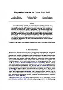
4 Results and discussions The prediction of the models on the test set are summarised in figure 1. We observe comparable performance of all three GLS regression techniques. In terms of RMSE, Ordinary Least Squares (OLS) which had the largest mean value showed that the validation data are badly fitted. The reason is that the OLS regression does not explicitly take into account the problems of multicollinearity and correlated error. Although the results achieved with GLS regression were superior to OLS, GLS poorly estimating the AR coefficients due to the influence of multicollinearity. Both PCR and PLSR can handle multicollinearity in the data, thus a large reduction of RMSE values were found for both techniques. We can see that the PLSR fitted slightly better 118
10 8 6
RMSE
4 2
OLS
GLS
PCR
GLS−PCR
PLS
GLS−PLSR
Figure 1: Comparison between the predictive performance of different regression methods
than PCR. This is probably due to the fact that the response variable is involved in the construction of PLSR components, contrary to the PCR components that only depend on the x-variables. Using GLS in PCR and PLSR the RMSE decreased drastically and resulted in average values close to the standard deviation of the simulated white noise. This further improvement reflected the fact that the underlying model and correlated error structure were appropriately estimated. Compared with GLS-PCR, the RMSE values are slightly in favour of GLS-PLSR.
References Amemiya, T., (1985). Advanced Econometrics. Harvard University Press, Cambridge. Greene, W.H., (2000). Econometric Analysis. Macmillan, New York. Luo, W., Baxter, P.D., & Taylor, C.C., 2006. Regression models for high dimensional data – a simulation. study In S. Barber, P.D. Baxter, K.V.Mardia, & R.E. Walls (Eds.), Interdisciplinary Statistics and Bioinformatics, pp. 128-131. Leeds, Leeds University Press. Ruud, P.A., 2000. An Introduction to Classical Econometric Theory, Oxford University Press, New York.
119