Regularisation Using Spatiotemporal Independence and Predictability

Regularisation Using Spatiotemporal Independence and Predictability JV Stoneand J Porrill

Psychology Department, Sheeld University, Sheeld, England, S30 2TP.

Abstract Independent component analysis (ICA) of an image sequence extracts a set of statistically independent images, and de nes a corresponding set of unconstrained dual time courses. However, the extra degrees of freedom implicit in these time courses can lead to physically improbable solutions. Accordingly, we introduce two methods for regularising ICA: smoothed independent component analysis (smICA), and spatiotemporal ICA (stICA). smICA is based on the observation that temporal signals tend to vary smoothly, and stICA is based on the observation that images and time courses tend to be statistically independent. A key feature of these methods is that they are based on generic physical properties, and may therefore be widely applicable. The methods are demonstrated on synthetic fMRI images.

1 Introduction Linear mixtures of signals have the following properties: 1) the central limit theorem ensures that they tend to be Gaussian, and 2), they are not statistically independent. Property 1 forms the basis of projection pursuit [2], whereas both properties 1 and 2 are critical assumptions underlying ICA [3]. However, a third property, predictability, almost always decreases if signals are mixed together. Speci cally, a given signal tends to be more predictable than a mixture of signals. For example, if each of two source signals is derived from a second order system then a linear mixture of them (usually) de nes a signal with fourth order properties. Like properties 1 and 2, the relatively high predictability of source signals is a generic consequence of mixing signals together. Whilst we conjecture that predictability could form the basis for extracting source signals, for the present, we demonstrate that it can be used to regularise solutions found by ICA. Additionally, we demonstrate that ICA can be regularised by imposing statistical independence constraints on the dual signals extracted by ICA. WWW: http : ==www:shef:ac:uk=~pc1jvs 

2 Spatial, Temporal and Spatiotemporal ICA ICA can be used in two complementary ways to decompose an image sequence into a set of images and a corresponding set of time-varying image amplitudes. Spatial ICA (sICA) [4] nds a set of mutually independent component (IC) images and a corresponding (dual) set of unconstrained time courses, whereas temporal ICA (tICA) [1] nds a set of IC time courses and a corresponding (dual) set of unconstrained images. Critically, for both sICA and tICA, the unconstrained nature of the dual signals permits them to adopt physically improbable forms in order to satisfy the constraint that their corresponding ICs are statistically independent. That is, ICA can contrive to nd statistically independent signals by making use of the extra degrees of freedom implicit in the unconstrained dual signals, even if the underlying sources are not statistically independent. ICA can therefore nd independent signals which are not the underlying sources. Thus, the independence of extracted (spatial or temporal) signals can be achieved at the cost of physically improbable forms for their unconstrained (temporal or spatial, respectively) dual signals. However, we can regularise solutions found with ICA by placing constraints on the dual signals. A natural modi cation to ICA consists of maximising the degree of independence between dual signals. Accordingly, we introduce spatiotemporal ICA (stICA). stICA places the ICs and their dual signals on an equal footing. The critical dierence between ICA (e.g. sICA, tICA) and stICA is as follows. ICA can achieve independence over space (sICA) or time (tICA) by `sacri cing' the dual temporal (sICA) or dual spatial (tICA) signals. In contrast, stICA maximises the degree of independence over space and time, without necessarily producing independence in either space or time. That is, stICA permits a trade-o between the mutual independence of images and the mutual independence of their corresponding time courses. Consider an m  n matrix containing a sequence of n images X = (x1 ; : : :; xn ). A linear decomposition into k modes is de ned by a matrix factorisation X = ST t , where S = (s1 j : : : jsk ), T = (t1 j : : : jtk ), and  is a diagonal matrix of scaling parameters. Image vectors si for spatial modes are represented in the columns of S, and their corresponding time courses ti are the columns of T. Brie y, spatial ICA nds independent images (columns) for S and a corresponding set of unconstrained time courses T, whereas temporal ICA nds independent time courses (columns) for T, and a corresponding set of unconstrained images S. It is convenient to reduce the rank of the problem using singular value decomposition (SVD). SVD provides a factorisation X  UDV t , where U is an m  k matrix of k  m eigenimages, V is an n  k matrix of k eigensequences, and D is a diagonal matrix of singular values. For later use, we de ne X~ = UDV t = U~ V~ t where U~ = UD1=2 and V~ = V D1=2. Spatial ICA: sICA embodies the assumption that U~ can be decomposed: U~ = SAS , where AS is an k  k mixing matrix, and S is an m  k matrix of k statistically ~ S. independent images. sICA can be used to obtain the decomposition yS = UW ? 1 WS is a permuted version of AS , such that each column in yS is a scaled version of exactly one column in S. This is achieved by maximising the entropy hS = H(YS ) of Y = (yS ), where  approximates the cdf of each of the spatial source signals.

Temporal ICA: tICA embodies the assumption that V~ can be decomposed: V~ = TAT , where AT is an k  k mixing matrix, and T is an m  k matrix of k statistically independent temporal sequences. tICA can be used to obtain the decomposition yT = V~ WT . WT is a permuted version of AS? , such that each column vector in yT is a scaled version of exactly one column vector in T. This is achieved by maximising the entropy hT = H(Y) of YT = (yT ), where  approximates the cdf 1

of the temporal source signals. Spatiotemporal ICA: stICA embodies the assumption that X~ can be decomposed: X~ = ST t , where S is an m  k matrix of k mutually independent images, T is an n  k matrix of mutually independent sequences, and  is a diagonal scaling matrix1. If X~ = U~ V~ t then two k  k unmixing matrices WS and WT exist such ~ S and T = V~ WT : that S = UW ~ S (V~ WT )t = UW ~ S WTt V~ t X~ = ST t = UW (1) If X~ = U~ V~ t = ST t then it follows that WT = (WS?1 )t (?1 )t. WS and WT can be found by simultaneously maximising a function hST of the spatial and temporal entropy of extracted signals. The temporal entropy is hT = H(YT ), where YT = (yT ) and yT = V~ WT is a set of extracted temporal signals. The spatial entropy ~ S is a set of extracted spatial is hS = H(YS ), where YS = (yS ) and yS = UW signals. The function h to be maximised is de ned: hST (WS ; ) = hS + (1 ? )hT (2) where  de nes the relative weighting aorded to spatial and temporal entropy, and where the latter are de ned as: Xm Xk log 0(yij ); h = log jW j + 1 Xn Xk log 0(yij ) (3) hS = log jWS j + m1 T T n i S i T j =1 i=1 j =1 i=1

The functions i and i are assumed to be the cdfs of the individual spatial and temporal signals, respectively, and their derivatives i0 and i0 are the corresponding pdfs. The functions de ned in Equation (3) have the same form as those in [1], and their derivatives can be obtained as described in that paper.

3 Smoothed ICA As discussed above, sICA places no constraints on the dual temporal signals. If the cdfs of source images are a poor approximation to the model cdfs (e.g. tanh) used in sICA or if the source images are not independent then the images recovered will be corrupted. However, if it is known that the dual temporal signals vary smoothly then this can be used to regularise the images recovered by sICA. Speci cally, the function hS can be augmented with a regularising function hP , which measures the degree of temporal smoothness, or predictability, in a dual temporal signal. Maximising the resultant function hSP nds solutions which represent a compromise between statistical independence of extracted images and temporal smoothness of one dual time course: hSP (WS ) = (1 ? ) hS + hP (4) 1  is required to ensure that S and T have amplitudes appropriate to their respective cdfs  and  .

where de nes the relative weighting given to spatial entropy hS and temporal smoothness hP . We restrict regularisation to the rst dual temporal signal yT = V~ wT , where wT is the rst row in WT = (WSt )?12. The regularising function hP is the log ratio of long-term variance to short-term variance of y: Pni=1(yi ? yi)2 1 (5) hP = 2 log Pn (~y ? y )2 i i=1 i The quantities y~i and y i are both temporal exponentially weighted sums: y~i = S y~(i?1) + (1 ? S ) yi?1 : 0  S  1 (6) y i = L y (i?1) + (1 ? L ) zi?1 : 0  L  1 (7) The half-life hL of L is much longer (typically 100 times longer) than the corresponding half-life hS of S . The derivative of Equation (5) is given in [6], where an information-theoretic interpretation of hP can also be found. Note that hP is invariant with resect to the magnitude of weights, and has the same form as Fisher's linear discriminant. The regularising function hP used here is a form of weak model [5]. A key feature of such models is that they specify only quite general properties of the dual signal.

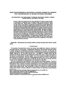
4 Results We synthesised data that were designed to emulate the gross properties of fMRI and optical imaging data (see Figure 1). The spatial sources S consisted of a set of four 40  40 pixel images S. These spatial sources were modulated with four corresponding sinusoidal time courses T (each of which was 1600 time steps) to form a 1600  1600 data set X = ST t , where each column of X is formed by concatenating rows in a single image. Three of the time courses are sinusoidal, and one consists of a sinusoid which is modulated by a linear ramp. In order to make results clear, each image contains an elliptical region which is unformly grey, and a circular region containing Gaussian noise. The overlapping regions with independent smooth and periodic time courses are typical of those found in biological data sets [5]. We applied principal component analysis (PCA) (using SVD) to the n = 1600 images in X. X was pre-processed so that each row and each column had zero mean, and SVD was used to obtain X~ = U~ V~ t , where columns of U~ and V~ contains the rst four eigenimages and eigensequences of X, respectively. For each method of extraction, solutions were obtained using a conjugate gradient method, and each run required about 1 minute on an SGI Indy R4400. All solutions are based on the same (random) unmixing matrix. The model pdf used to evaluate hS (for stICA and sICA) was 0 = (1 ? tanh2), and the model pdf used to evaluate hT (for stICA) was  0 = exp(?x4). PCA: The eigenimages and eigensequences of X contain linear mixtures of their respective source signals (not shown). sICA: The source images are not recovered, and that their dual time courses are corrupted, as shown in Figure 2. 2

The scaling matrix  is not required for smICA.

tICA: Each extracted time course is a linear mixture of the source time courses, and the recovered images are similarly corrupted, as shown in Figure 3. (Note that removal of the linear ramp from IC1 of Figure 1 permits near perfect recovery of sources). stICA: With stICA, the inclusion of temporal entropy hT essentially regularises the solution found by sICA. Using a low-kurtosis model cdf  for hT , and  = 0:5, the source signals are recovered almost perfectly, as shown in Figure 4. smICA: As shown in Figure 5, smICA almost perfectly extracted a spatial IC (IC3 in Figure 1) and its dual time course. Extracting one IC correctly has the eect of constraining the remaining spatial ICs, such that another of the original image sources (IC4 in Figure 1) and its dual time course were also recovered. Note that the two recovered source images have a large degree of spatial overlap. The remaining extracted images are poorly de ned. A short-term half-life of 4 time steps, and a long-term half-life of 4000 was used, with = 0:5. The solution found is insensitive to the value of the short-term half-life. We also regularised tICA by applying the smoothness constraint hP to one temporal signal extracted by tICA (not shown). As with smICA, which regularises sICA, the regularised temporal mode was a good approximation of one of the original sources. Whilst in this particular case, regularising one extracted temporal signal with hP is quite consistent with the form of the underlying temporal source signal, this may be not true in general. Finally, and as conjectured in the Introduction, simply maximising predictability hP has been used by us to extract a single speaker's voice from two or more mixtures of speakers' voices.

5 Discussion Uniquely, stICA is based on the assumption that both spatial and temporal signals are independent. This assumption is rarely valid, so that stICA provides solutions in which the degree of spatial independence is maximised subject to the constraint that the degree of temporal independence is maximised (and vice versa). Essentially, stICA is based on the physically realistic assumption that both spatial and temporal sources are almost independent. Such sources are likely to exist in a classically spatiotemporal medium such as brain tissue, in which correlations in activity between nearby points in space and time are the norm. Such considerations make stICA a potentially powerful tool for a functional decomposition of brain activity. We conjecture that the assumptions on which ICA is based are frequently violated in practice. We have demonstrated that the addition of prior knowledge in the form of physically realistic constraints can be used to minimise the consequences of such violations.

Acknowledgments JV Stone is a Wellcome Mathematical Biology Research Fellow.

Spatial IC #1

Spatial IC #2

Temporal IC #1

Temporal IC #2

Spatial IC #3

Spatial IC #4

Temporal IC #3

Temporal IC #4

Figure 1: Original spatial and temporal sources. Spatial IC #1

Spatial IC #2

Temporal IC #1

Temporal IC #2

Spatial IC #3

Spatial IC #4

Temporal IC #3

Temporal IC #4

Figure 2: Spatial ICA: Extracted spatial modes, and dual temporal modes.

References [1] AJ Bell and TJ Sejnowski. An information-maximization approach to blind separation and blind deconvolution. Neural Computation, 7:1129{1159, 1995. [2] JH Friedman. Exploratory projection pursuit. J Amer. Statistical Association, 82(397):249{266, 1987. [3] C Jutten and J Herault. Independent component analysis versus pca. In Proc. EUSIPCO, pages 643 { 646, 1988. [4] MJ McKeown, S Makeig, GG Brown, TP Jung, SS Kindermann, and TJ Sejnowski. Spatially independent activity patterns in functional magnetic resonance imaging data during the stroop color-naming task. Proceedings of the National Academy of Sciences USA., 95:803{810, Feburary 1998. [5] J Porrill, JV Stone, JEW Mayhew, J Berwick, and P Coey. Analysis of optical imaging data using weak models. In Human Brain Mapping (Dusseldorf, 1999). [6] J V Stone. Learning perceptually salient visual parameters through spatiotemporal smoothness constraints. Neural Computation, 8(7):1463{1492, 1996.

Spatial IC #1

Spatial IC #2

Temporal IC #1

Temporal IC #2

Spatial IC #3

Spatial IC #4

Temporal IC #3

Temporal IC #4

Figure 3: Temporal ICA: Extracted temporal modes and dual spatial modes. Spatial IC #1

Spatial IC #2

Temporal IC #1

Temporal IC #2

Spatial IC #3

Spatial IC #4

Temporal IC #3

Temporal IC #4

Figure 4: Spatiotemporal ICA: Extracted spatial and temporal modes. Spatial IC #1

Spatial IC #2

Temporal IC #1

Temporal IC #2

Spatial IC #3

Spatial IC #4

Temporal IC #3

Temporal IC #4

Figure 5: Spatial ICA with regularised dual temporal mode (#1).