Bayesian Analysis (2014)
9, Number 1, pp. 171–196
Regularized Bayesian Estimation of Generalized Threshold Regression Models Friederike Greb ∗ , Tatyana Krivobokova † , Axel Munk and Stephan von Cramon-Taubadel §
‡
,
Abstract. In this article we discuss estimation of generalized threshold regression models in settings when the threshold parameter lacks identifiability. In particular, if estimation of the regression coefficients is associated with high uncertainty and/or the difference between regimes is small, estimators of the threshold and, hence, of the whole model can be strongly affected. A new regularized Bayesian estimator for generalized threshold regression models is proposed. We derive conditions for superiority of the new estimator over the standard likelihood one in terms of mean squared error. Simulations confirm excellent finite sample properties of the suggested estimator, especially in the critical settings. The practical relevance of our approach is illustrated by two real-data examples already analyzed in the literature. Keywords: empirical Bayes, regularization, threshold identification
1
Introduction
Modeling a response variable as a linear combination of some covariates with regression coefficients that vary between (possibly several) regimes is known as threshold regression. The choice of regime is determined by a transition function, which depends on a transition variable as well as a threshold parameter. Transition functions can be either smooth (Van Dijk et al. 2002, provide a comprehensive overview) or step functions. In the following, we restrict attention to the latter. In principle, the response variable can follow any distribution from the exponential family. However, such generalized threshold regression models have only recently been formally introduced by Samia and Chan (2011), and most of the literature on threshold regression deals with models with a piecewise linear mean. In this article we concentrate on generalized regression models with regimes controlled by a step transition function and refer to such models as generalized threshold regression models. Generalized threshold regression models are employed in a wide range of different fields ∗ Department of Agricultural Economics and Rural Development and Courant Research Centre “Poverty, Equity and Growth in Developing Countries”, Georg-August-Universit¨ at G¨ ottingen, Germany
[email protected] † Courant Research Centre “Poverty, Equity and Growth in Developing Countries” and Institute for Mathematical Stochastics, Georg-August-Universit¨ at G¨ ottingen, Germany
[email protected] ‡ Institute for Mathematical Stochastics, Georg-August-Universit¨ at G¨ ottingen, and Max Planck Institute for Biophysical Chemistry, G¨ ottingen, Germany
[email protected] § Department of Agricultural Economics and Rural Development, Georg-August-Universit¨ at G¨ ottingen, Germany
[email protected]
© 2014 International Society for Bayesian Analysis
DOI:10.1214/13-BA850
172
Regularized Bayesian Estimation of GTRMs
of application. Hansen (2011) provides an overview of the extensive use of generalized threshold regression models in economic applications including e.g. models of output growth, forecasting, and the term structure of interest rates or stock returns. Samia et al. (2007) employ a generalized threshold regression model to analyze plague outbreaks, and Lee et al. (2011) complement these applications with examples in finance, sociology, and biostatistics among others. Obviously, a good threshold estimator is crucial for the entire threshold regression model estimation. In this paper we discuss settings in which threshold identification becomes difficult. Typically, threshold parameters are estimated by the maximization of the corresponding profile likelihood using a grid search, as the likelihood function is not differentiable with respect to the threshold parameter. This estimation procedure itself has an intrinsic problem: the profile likelihood is not defined for thresholds that leave fewer observations in one of the regimes than are necessary to estimate the regression coefficients. Hence, in practice it is unavoidable to restrict the domain of the threshold parameters depending on the dimension of the regression coefficients. The literature offers arbitrary constraints including one observation per dimension of the regression coefficient (Samia and Chan 2011) or 15% of the observations (Andrews 1993) to give just two examples. This restriction can be problematic in small samples, especially if the true threshold is close to the boundary of its domain. Another problem occurs if the threshold parameter itself lacks identifiability. In particular, if differences between regimes are small and/or the regression coefficients’ estimators are highly variable, the uncertainty of the threshold estimator increases. Note that the large variance of the regression coefficients’ estimator is likely to be found in small samples, for the true threshold at the boundary of its domain and also if the signal-to-noise ratio is low. We are not aware of any work that points out these deficiencies of the common threshold estimator even though the problematic settings frequently occur in empirical applications. Macro-economic data are often only available for a small sample, e.g. if observations correspond to different countries. Spatial arbitrage modeling is another example (Greb et al. 2013). Bayesian methods are also popular to estimate threshold regression models. In the literature Bayesian estimation is typically based on non-informative priors, leading to what we refer to as the non-informative Bayesian estimator. For the threshold estimator in the case of a threshold regression model with piecewise linear mean, Yu (2012) shows that, regardless of the choice of priors, Bayesian threshold estimators are asymptotically efficient among all estimators in the locally asymptotically minimax sense. However, in the critical small sample settings described above, the non-informative Bayesian estimator shares all the drawbacks of the standard likelihood estimator and can completely fail in certain cases, as we discuss in Section 3.2. In this article, we suggest an alternative estimator, which we call the regularized Bayesian estimator. Contrary to previous work on estimation in threshold regression (Samia and Chan 2011; Yu 2012), we focus on the estimator’s performance in critical small sample situations. Simulations confirm that it yields good results even in settings in which likelihood and non-informative Bayesian estimators are highly susceptible to
F. Greb, T. Krivobokova, A. Munk, and S. von Cramon-Taubadel
173
faults. Given the threshold parameter’s crucial function within the model, our idea is to improve estimation of the whole model by improving estimation of this essential parameter. To summarize the intuition for the new threshold estimator: If regression coefficients were known, none of the problems in threshold estimation outlined above would exist. This suggests that stabilizing their estimates might help to prevent them from distorting the threshold estimates. In addition, regularization of regression coefficient estimates allows us to obtain a posterior density that is well-defined on the entire domain of the threshold parameters. We achieve regularization by a particular specification of priors. While it proves to be beneficial in the critical small sample situations, the choice of priors does not have an impact asymptotically (as Yu 2012 shows for a threshold regression model with piecewise linear mean and independent observations). We further derive an explicit (approximate) expression of the posterior density, which allows us to utilize existing functions for mixed models in standard software to easily compute the threshold estimator and simultaneously obtain estimates for the remaining model parameters. The rest of this article is organized as follows. We specify the generalized threshold regression model in the second section. In the third section, we review existing estimators for threshold regression models and point out their deficiencies. Here, we concentrate on estimators for the crucial threshold parameter. The regularized Bayesian estimator is introduced in the fourth section. In the fifth section, we derive conditions under which the regularized Bayesian estimates fare better than their likelihood counterparts. Simulation results are presented in the sixth section. We use the last section to discuss two empirical applications. The appendix contains some technical details.
2
Model
( ) Observations yi , XTi , qi ∈ R × Rp × R, i = 1, . . . , n, are assumed to be realizations of random variables that follow a generalized threshold regression model with threshold parameter ψ ∈ R, regression coefficients β 1 , β 2 ∈ Rp and scale (or dispersion) parameter ϕ ∈ R+ , that is ( ) µi = E yi |XTi , qi = h(ηi ) (1) where h is a known one-to-one function, the inverse of the link function g = h−1 , and ηi = I (qi ≤ ψ) XTi β 1 + I (qi > ψ) XTi β 2 ,
(2)
with I(·) as the indicator function. Moreover, conditional on the design vector XTi and the transition variable qi , the response variables yi are independently drawn from an exponential family distribution with density } { yi θi − b(θi ) + c(yi , ϕ) , (3) f (yi |ψ, ϕ, β 1 , β 2 ) = exp ϕ characterized by known functions b and c together with the natural parameter θi = θ(µi ).
174
Regularized Bayesian Estimation of GTRMs
Above and in the following, the same symbol denotes both a random variable and its realization; the context should eliminate ambiguities. To use matrix notation, we define vectors µ, η, y, q, I(q ≤ ψ) and I(q > ψ) by stacking µi , ηi , yi , qi , I(qi ≤ ψ) and I(qi > ψ), respectively, and create an n × p matrix X with rows XTi , i = 1, . . . , n. With diag {I(·)} the diagonal matrix with entries I(·) along the diagonal and β = (β T1 , β T2 )T , we can write η = diag {I(q ≤ ψ)} Xβ 1 + diag {I(q > ψ)} Xβ 2 = X1 β 1 + X2 β 2 = Xψ β. We consider generalized threshold regression models with one threshold to keep the exposition simple; extension to generalized threshold regression models with more thresholds is straightforward (see e.g. Greb et al. 2013). Naturally, our model covers yi = I (qi ≤ ψ) XTi β 1 + I (qi > ψ) XTi β 2 + εi , εi ∼ N (0, s) and i = 1, . . . , n. This is by far the most frequently encountered generalized threshold regression model in the literature. It is broad enough to comprise the popular threshold autoregressive model in which the transition variable qi is an element of Xi (see Tong and Lim 1980; Tong 2011, for a review of the development of the model). Depending on the assumptions on the data generating process, inferences (or estimators) for model (1) – (3) can take on different asymptotic behavior. A first differentiation regards the transition variable qi . Change point models are characterized by deterministic qi = i, while for threshold models qi is a random variable which follows any continuous distribution. This is reflected in distinct limit likelihood ratio processes and, hence, asymptotic behavior of the maximum likelihood estimators for ψ in the two models. The limiting likelihood ratio process involves a functional of random walks for change point models and of compound Poisson processes for threshold models. Check Bai (1997) for more details on the asymptotic properties in the former, and Samia and Chan (2011) for the limiting behavior of the profile log-likelihood and the asymptotic distribution of the profile likelihood threshold estimator in the latter case. If the transition variable coincides with one of the covariates and the regression function is continuous at the threshold, least squares estimates are known to be normally distributed (for threshold models, see Chan and Tsay 1998; Feder 1975 treats change-point models), which simplifies inference. Clearly, once the data is sampled, the estimation procedure in both change point and threshold models is the same. Referring to a threshold regression model with piecewise linear mean, Hansen (2000) points out that “if the observed values of qi are distinct, the parameters can be estimated by sorting the data based on qi , and then applying known methods for change point problems”. As the focus of this article is on estimation problems that arise in small samples, we do not further differentiate between models. In the real-data examples, we concentrate on discontinuous threshold models since they are frequently encountered in applications and have not been studied as extensively as change point models due to their more intricate limiting behavior.
F. Greb, T. Krivobokova, A. Munk, and S. von Cramon-Taubadel
3 3.1
175
Estimation of threshold regression models The likelihood estimator
As noted in the introduction, the prevalent estimator of threshold regression models is the likelihood estimator, see e.g. Samia and Chan (2011) or Hansen (2000). Thereby, the threshold parameter is estimated from the corresponding profile likelihood Lp , which is constructed from the likelihood function L, by replacing nuisance parameters β T ∈ R2p and ϕ ∈ R with their maximum likelihood estimates at given values of ψ (which are just standard (weighted) least squares estimators). More specifically, we work with the conditional profile likelihood function given X and q, [ n { }] n ∏ ∑ yi θˆi − b(θˆi ) ˆ ˆ ˆ Lp (ψ) = f (yi |ψ, ϕψ , β ψ ) = exp + c(yi , ϕψ ) , ϕˆψ i=1 i=1 [ { }] ˆ1 + I(qi > ψ)XTi β ˆ2 ˆψ and ϕˆψ are where θˆi = θ {h(ˆ ηi )} = θ h I(qi ≤ ψ)XTi β and β ψ ψ maximum likelihood estimators at a fixed ψ. In the following, we assume a canonical link, that is, θi = ηi . All developments still hold approximately if this assumption does not hold. We denote the profile log-likelihood with ℓp (ψ) = log Lp (ψ). In generalized threshold regression{ models, the domain of } the threshold parameter ψ is restricted to a random set Ψ = ψ ∈ R|q(1) ≤ ψ ≤ q(n) ⊆ R, where q(i) denotes the ith order statistic. To measure the proximity of a threshold ψ to the boundary of its domain Ψ, we introduce d(ψ) = min(j, n − j)/p with j such that q(j) ≤ ψ < q(j+1) . The quantity d(ψ) is the distance between ψ and Ψ’s boundary in terms of the number of observations between them relative to the dimension of the regression coefficients, p = dim (β k ), k = 1, 2. When d(ψ) = 1, ψ assigns at least p observations to each of the regimes. The allocation of 5% of the observations into one of the regimes can be expressed as d(ψ) = 0.05 n/p. Clearly, Lp (ψ) is not defined for d(ψ) < 1, since in this case ψ does not leave enough observations for the estimation of β k in one of the regimes. Hence, in practice it is inevitable to restrict Ψ to Ψ∗ (c) = {Ψ| d(ψ) > c} for some c ≥ 1. In the literature different heuristic suggestions for the choice of c have been proposed. For example, Hansen and Seo (2002) propose c = 0.05 n/p, we find c = 0.15 n/p in Andrews (1993) and Samia and Chan (2011) even use c = 0.25 n/p for their application. The profile likelihood threshold estimator is then given by ψˆpL = argmax Lp (ψ). ψ∈Ψ∗ (c)
This definition based on the restricted domain Ψ∗ (c) immediately suggests that in settings in which d (ψ0 ) < c for a true threshold ψ0 , ψˆpL is inconsistent. The left panel of Figure 1 illustrates this showing the profile log-likelihood for a sample run of a generalized threshold regression model corresponding to the simulation setting 1C detailed in Section 6. If Ψ∗ (1) = [0.3, 0.7] would be restricted any further, e.g. to be [0.31, 0.69],
176
Regularized Bayesian Estimation of GTRMs Noninformative Bayes ψ0 = 0.3 4
10
Regularized Bayes ψ0 = 0.3
0.0
0.2
0.4
0.6
0.8
1.0
0
0
0
2
1
2
4
2
4
6
3
8
6
8
Profile likelihood ψ0 = 0.3
0.0
ψ
0.2
0.4
0.6
ψ
0.8
1.0
0.0
0.2
0.4
0.6
0.8
1.0
ψ
Figure 1: For a sample run corresponding to setting 1C of Section 6, ℓp (ψ) is shown on the left, log pnB (ψ|y, X, q) in the middle and log prB (ψ|y, X, q) on the right. then the true threshold ψ0 = 0.3 would be excluded from the threshold domain and ψˆpL would move to the next extremum. For small n, large p and ψ0 close to the boundary of Ψ, d (ψ0 ) < c is likely to be the case. Altogether, subjective restriction of the threshold domain is an undesirable property of threshold estimation based on the profile likelihood. The same plot in Figure 1 also exemplifies that in certain small-sample settings the profile (log-)likelihood can be jagged and have multiple extrema, leading to an estimated ˆψ threshold that is very sensitive to the initialization of the search. Large variance of β and/or small differences between regimes compared to the noise level can have a strong distorting effect on the profile (log-)likelihood and are associated with settings characterized by small n relative to p, but can also be due to low signal-to-noise ratio, model misspecifications (e.g. overdispersion), or a threshold that is close to the boundary of its domain. This is exposed in the left as compared with the middle plot of Figure 2; the log-likelihoods depicted in these plots belong to models which only differ in one aspect: in the plot on the left-hand side, the residual standard deviation is 0.75, while ˆψ ). Clearly, the in the middle plot it is 1.5, increasing the signal-to-noise ratio and var(β log-likelihood in the middle plot is highly distorted over the whole range of Ψ, triggering multiple extrema and a highly variable estimator for ψ. Moving the true threshold closer to the boundary, as shown in the right plot of Figure 2, leads to an even stronger deformation of the log-likelihood. In summary, in small samples and particular settings exemplified above, the profile likelihood threshold estimator can perform poorly, being very sensitive to inappropriate estimates of the nuisance parameters and relying on a subjective restriction of its domain.
3.2
The Bayesian estimator
For threshold regression models with piecewise linear mean, there is a long tradition of using Bayesian techniques in applied work beginning with Bacon and Watts (1971) and
F. Greb, T. Krivobokova, A. Munk, and S. von Cramon-Taubadel Setting 1 B
15
30
Setting 1 A
Setting 1 C ψ0 = 0.3
6
5
2
10
5
4
15
20
10
25
8
ψ0 = 0.5
177
0.2
0.4
0.6
ψ
0.8
1.0
0
0
0
ψ0 = 0.5 0.0
0.0
0.2
0.4
0.6
ψ
0.8
1.0
0.0
0.2
0.4
0.6
0.8
1.0
ψ
Figure 2: Sample (log) profile likelihood functions ℓp (ψ) for different settings.
including Geweke and Terui (1993) among many others. This popularity can be at least partially attributed to practical advantages, since the Bayesian approach offers a natural framework for inference and accounts for the uncertainty of the nuisance parameters. The Bayesian regression coefficients estimators coincide with the maximum likelihood ones for non-informative priors. The theoretical properties of Bayesian threshold estimators in certain generalized threshold regression models have been investigated by Yu (2012). He shows that for independently and identically distributed observations Bayesian threshold estimators are asymptotically efficient among all estimators in the locally asymptotically minimax sense and strictly more efficient than the maximum likelihood estimator. In a related paper, Chan and Kutoyants (2012) examine asymptotic properties of Bayesian estimators in threshold autoregression models. They note that in the limit, the variance of the Bayesian estimator is smaller than that of the maximum likelihood estimator. Without any prior knowledge of possible parameter values, it is natural to assume a uniform prior for the threshold parameter and non-informative priors for the regression coefficients; these choices are (almost) omnipresent in the Bayesian literature on generalized threshold regression models with piecewise linear mean. While the priors do not have an impact asymptotically, it turns out that they do affect the performance of the Bayesian threshold estimator in finite samples. We show that non-informative priors can distort estimates, especially in small samples. It is straightforward to obtain an approximation of a generalized threshold regression model’s posterior density pnB (ψ|ϕ, y, X, q) associated with non-informative (improper) priors p(β) ∝ 1 and p(ψ|q) ∝ I(ψ ∈ Ψ) based on a Laplace approximation (Shun and McCullagh 1995; Severini 2000) of the integral for fixed p ≪ n ∫ R2p
) −1/2 ( ) ∂2ℓ ( ˆψ ψ, ϕ, β + O n−1 , p(y|ψ, ϕ, β, X, q)dβ = Lp (ψ)(2π)p − T ∂β∂β
178
Regularized Bayesian Estimation of GTRMs / ( ) ˆψ = X Tψ WX ψ , we get with ℓ(ψ, ϕ, β) = log L(ψ, ϕ, β). As −∂ 2 ℓ ∂β∂β T ψ, ϕ, β −1/2 ) ( pnB (ψ|ϕ, y, X, q) = Lp (ψ)(2π)p X Tψ WX ψ I(ψ ∈ Ψ)/p(y) + O n−1 . With this, the prevalent Bayesian threshold estimator in the literature is the poste∫ rior mean ψˆnB = ψpnB (ψ|ϕ, y, X, q)dψ. Comparing pnB (ψ|ϕ, y, X, q) with Lp (ψ), Ψ∗ −1/2 we note that they differ by a term proportional to X Tψ WX ψ . In the case of Gaussian observations, W = I n /σ 2 . Since X Tψ WX ψ = XT1 WX1 · XT2 WX2 → 0 for d(ψ) → 0, pnB (ψ|ϕ, y, X, q) becomes very large for ψ close to the boundary of Ψ. Moreover, as the profile likelihood function requires d(ψ) ≥ 1 to be well-defined, so does the calculation of the posterior density. Again, the only solution in the literature is to restrict the parameter space Ψ (which in our Bayesian framework is equivalent to working with a uniform prior ψ ∼ U [Ψ∗ ] instead of ψ ∼ U [Ψ]). In this case, however, pnB (ψ|ϕ, y, X, q) becomes largest exactly for values of ψ which are arbitrarily included or excluded from Ψ∗ by varying c. Consequently, expanding or reducing Ψ∗ critically affects the Bayesian threshold estimate, whether it is calculated as the posterior mode, mean or median. The middle plot in Figure 1 illustrates this problem.
4
The regularized Bayesian estimator
When rethinking the threshold regression estimation, there are good arguments for continuing to pursue Bayesian options. In general, Bayesian estimators naturally incorporate the uncertainty of nuisance parameters and there are reasons to expect the threshold estimators to be (at least asymptotically) the most efficient estimators, as discussed in Section 3.2. Our idea now is to exploit understanding of when reliable estimation becomes particularly difficult in order to regularize the posterior density. First, we define η = X1 β 1 + X2 β 2 = (X1 + X2 )β 1 + X2 (β 2 − β 1 ) = Xβ 1 + X2 δ.
(4)
Here, X is independent of ψ, while X2 = X2 (ψ) = diag {I(q > ψ)} X. Hence, if δ is small and/or its estimators are highly variable, it becomes hard to identify the threshold ψ. We, therefore, suggest to regularize the estimator for δ. In a Bayesian framework the natural approach is to assume δ ∼ N (0, σδ2 I p ). When σδ2 tends towards infinity, this prior becomes non-informative. However, for small values σδ2 , we introduce prior knowledge suggesting that δ takes values close to zero, that is there is no threshold in the model. The most important characteristic of this new choice of priors is that it regularizes the posterior density for ψ close to the boundary of Ψ. Putting priors on σδ2 (e.g. an inverse Gamma distribution) and ψ specifies a fully Bayesian model and allows for estimation with Markov chain Monte Carlo techniques. Alternatively, we suggest to use a Laplace approximation to get the approximate posterior p(ψ|ϕ, σδ2 , y, X, q). This accelerates estimation and enables us to illustrate the
F. Greb, T. Krivobokova, A. Munk, and S. von Cramon-Taubadel
179
regularizing effect. To evaluate the posterior density p(ψ|ϕ, σδ2 , y, X, q)
p(ψ|q) = p(y|ϕ, σδ2 , X, q)
∫ ∫ p(y|β 1 , δ, ψ, ϕ, σδ2 , X, q)p(δ|σδ2 )dδdβ 1 , Rp Rp
we use a Laplace approximation and follow a line of reasoning closely resembling Breslow and Clayton (1993) to obtain ∫ ∫ p(y|β 1 , δ, ψ, ϕ, σδ2 , X, q)p(δ|σδ2 )dδdβ 1 Rp Rp
} n ∑ 1 −1 T ˆ ˆ z − Xβ 1 ) V (˜ z − Xβ 1 ) + exp − (˜ c(yi , ϕ) (5) 2 i=1 −1/2 T −1 −1/2 ( ) X V X · σδ2 XT2 WX2 + I p + O n−1 , {
= (2π)
p/2
ˆ1 + X2 dˆ + G(y − µ), G = diag {g ′ (µi )}, ˜ defined as z ˜ = X{ with the working variable z β } −1 −1 2 T and V = W + σδ X2 X2 for W = diag ϕb′′ (θi )g ′ (µi )2 . Here, µ, G, W and V are evaluated at the (approximate) posterior mode ˆ = arg max(β ,δ)∈R2p p(β , δ|ψ, ϕ, σ 2 , y, X, q), that is, ˆ1 , d) (β 1 δ 1 ˆ1 ). Note that these regression ˆ ˜ and dˆ = σδ2 XT2 V −1 (˜ z − Xβ β 1 = (XT V −1 X)−1 XT V −1 z parameter estimators are regularized and are different from usual likelihood estimators. Details on the derivation of (5) are provided in the appendix. In contrast to the posterior based on non-informative priors, the term |X Tψ WX ψ | disappears, and with it the deteriorations near the boundary of Ψ observed for pnB (ψ|ϕ, y, X, q). Moreover, p(ψ|ϕ, σδ2 , y, X, q) is well-defined for all ψ ∈ Ψ, indepenˆ1 → (XT WX)−1 XT W˜ dent of d(ψ). It is easy to see that dˆ → 0 and β z at the boundary of Ψ, for X2 = 0 or X2 = X. We do not encounter the ill-posed problem of estimating ˆψ when d(ψ) < 1, as p nuisance parameters from m < p observations, or calculating β in profile likelihood or non-informative Bayesian estimation. Consequently, there is no need to subjectively restrict the parameter space. Considering ˆ1 ) dˆ =σδ2 XT2 V −1 (˜ z − Xβ
(6)
ˆ1 − X2 δ)T W(˜ ˆ1 − X2 δ) + 1 δ T δ, = arg min (˜ z − Xβ z − Xβ p σδ2 δ ∈R it becomes evident that the proposed prior leads to the strategy of turning an ill-posed into a well-posed problem tracing back to Tikhonov et al. (1977). For small values of the regularization parameter 1/σδ2 , the first term of the functional to be minimized in (6) ˆ for large values it is the latter. For the nuisance parameter estiwill drive the resulting d, ˆ basic matrix algebra reveals that β ˆ1 and β ˆ2 = β ˆ1 + d, ˆ1 → (XT1 WX1 )−1 XT1 W˜ mates β z T −1 T 2 2 ˆ2 → (X2 WX2 ) X2 W˜ ˆ1 and β ˆ2 converge and β z for σδ → ∞, while for σδ → 0, both β to (XT WX)−1 XT W˜ z.
180
Regularized Bayesian Estimation of GTRMs
Clearly, the choice of the regularization parameter σδ2 is essential to any estimate based on p(ψ|ϕ, σδ2 , y, X, q). It can naturally be estimated in the fully Bayesian framework. However, pursuing our approximate approach further we prefer to make use of the empirical Bayes paradigm. In general, the empirical Bayes approach to modeling observations y differs from the usual Bayesian setup in that the hyperparameters for the highest level in the model’s hierarchy are replaced by their maximum likelihood estimates. In our case, we obtain σ ˆδ2 for fixed X, q and ψ by maximizing ∫ ∫ p(y|β 1 , δ, ψ, ϕ, σδ2 , X, q)p(δ|σδ2 )dδdβ 1 , p(y|ψ, ϕ, σδ2 , X, q) = Rp Rp
so as to base threshold estimation on prB (ψ|y, X, q) =
−1/2 −1/2 T ˆ −1 2 T ˆδ X2 WX2 + I p ∝ σ X V X { } n ( ) ∑ −1 1 ˆ1 )T Vˆ (˜ ˆ1 ) + · exp − (˜ z − Xβ z − Xβ c yi , ϕˆψ I(ψ ∈ Ψ), 2 i=1
p(ψ|y, X, q, ϕˆψ , σ ˆδ2 )
with Vˆ evaluated at σ ˆδ2 . The right plot in Figure 1 shows the log of this posterior density for a sample run corresponding to simulation setting 1 C of Section 6. It is clearly welldefined over the whole domain of the threshold and its values are regularized at the boundary regions, making the extremum more pronounced. Once the posterior density is obtained, one can calculate ψˆrB . We observed that in critical small-sample settings the posterior density is often characterized by multiple modes. Thus, obtaining an estimate based on numerical maximization (the posterior mode) is likely to be challenging. The posterior mean presents a more robust alternative. However, when the true threshold is located close to the boundary of Ψ, the posterior distribution is skewed towards this boundary. As a result, the posterior mean tends to be drawn towards the middle of Ψ (Doodson 1917; Kendall 1943, page 35). Hence, we opt for the posterior median as a compromise between the latter two. Accordingly, we suggest calculating a regularized Bayesian threshold estimator ψˆrB as ψ ∫ˆrB
prB (ψ|y, X, q, ϕ)dψ = 0.5 q(1)
assuming a prior p(ψ|q) ∝ I(ψ ∈ Ψ) for ψ. By definition, the restricted (or residual) likelihood function (Harville 1977) of a generalized linear mixed model is the approximate posterior (5). Hence, the function glmmPQL in the R-package MASS readily provides us with the desired estimate σ ˆδ2 . Moreover, the function simultaneously produces an estimate ϕˆψ . For the Gaussian case, we can employ the function lme directly (with its parameter method left at the default value REML). It is part of the R-package nlme. This possibility to take advantage of existing
F. Greb, T. Krivobokova, A. Munk, and S. von Cramon-Taubadel
181
functions implemented for mixed models greatly facilitates computation of our proposed estimator, which can be performed in seconds. Inference about all of the model parameters naturally follows in this Bayesian framework. In particular, confidence regions for ψ are formed as credible sets; an equi-tailed credible set C of level 1 − 2α is defined as ∫
qp (1−α)
C=
p(ψ|y, X, q, ϕ)dψ, qp (α)
∫ p(ψ|y, X, q, ϕ)dψ ≥ α . qp (α) = inf x x∈Ψ ψ≤x
These credible sets are valid for change-point and threshold models, both continuous and discontinuous. By contrast, in the frequentist framework it is straightforward to obtain confidence intervals for continuous models. For discontinuous models the asymptotic distribution does not readily provide a feasible way to construct confidence intervals as it depends on (a possibly large number of) nuisance parameters.
5
Comparison of regularized Bayesian and maximum likelihood estimation
Our new estimation procedure results in new regularized regression coefficients estimators, whose properties have not been investigated so far. In the following, we compare regularized Bayesian and maximum likelihood approaches to estimation of threshold regression models in terms of mean squared error under the frequentist model. Thereby, we treat the threshold as fixed and known, but allow for any, not necessarily true threshold ψ. A natural measure for comparing coefficient estimates is the mean squared error ( )T ( ) ˆ = E Xψβ ˆ − Xψβ ˆ − X ψ β , where E denotes the conditional exM(X ψ β) Xψβ pectation without averaging over the prior assumptions, i.e. expectation with respect to the distribution of Y given δ, which corresponds to the usual frequentist framework. In the context of ridge regression, this approach has been criticized for indiscriminately putting together the mean squared errors of the components (Nelder 1972; Theobald 1974). As an alternative, Theobald (1974) suggested to consider a weighted sum ( )T ( ) ˆ = E Xψβ ˆ − Xψβ A Xψβ ˆ − X ψ β for a non-negative definite matrixA. MA (X ψ β) ˆ (or Here, ψ is an arbitrary, fixed threshold. Of course, a comparison between M(X ψ β) ˆ for different β ˆ is both interesting for such general ψ as well as the true MA (X ψ β)) threshold ψ0 . With this in mind, we state the following result. T −1 ˆ Theorem 1 For maximum likelihood estimates β X ψ Wz and regM L = (X ψ WX ψ ) T −1 ˆ = (X WX ψ +H) X ψ Wz of β based on a threshold ularized Bayesian estimates β rB ψ ψ ≤ ψ0 , ψ0 the true threshold,
182
Regularized Bayesian Estimation of GTRMs ( ) ( ) ˆ ˆ MA X ψ β Xψβ ≥ 0 for all non-negative definite matrices A M L −MA rB
(i) ⇔
{ } ( ) D (I + C) H − (B + H) ββ T BT + H + CBββ T BT CT DT is non-negative definite.
(ii)
( ) ( ) ˆ ˆ M Xψβ − M Xψβ ≥0 ML rB { } ⇔ tr HDT D (I + C) {( ) } − β T BT + H DT D (B + H) + BT DT0 D0 B β ≥ 0.
{ } Here, W−1 (= diag ϕb′′)(θi )g ′ (µi )2 , G = diag {g ′ (µi )}, and z = X ψ β + G(y − µ), ( )−1 ( )−1 I p −I p H = 1/σδ2 , D = X ψ X Tψ WX ψ + H , D0 = X ψ X Tψ WX ψ , −I p I p ) ( ( )−1 0 0 with C = I + H X Tψ WX ψ , and B = −X T[ψ,ψ0 ] WX [ψ,ψ0 ] X T[ψ,ψ0 ] WX [ψ,ψ0 ] X [ψ,ψ0 ] = diag{I(ψ < q ≤ ψ0 )}X. Remark 1 For the Gaussian model with W = 1/sI n and at the true threshold ψ = ψ0 , equivalence (i) reduces to ( ) ( ) ˆ ˆ MA X ψ β − M X β ψ rB ≥ 0 for all non-negative definite matrices A ML A δ T (2σδ2 /sI + Z)−1 δ ≤ s,
⇔
where Z = (XT1 X1 )−1 + (XT2 X2 )−1 , while equivalence (ii) reduces to ( ) ( ) ˆ ˆ M Xψβ − M X β ≥0 ψ ML rB { ( ) ( )−2 } −2 ⇔ δ T Z s/σδ2 I p + Z δ ≤ s p − tr I p + s/σδ2 Z .
(7)
(8)
Remark 2 Using a singular value decomposition Z = U diag (η1 , . . . , ηp ) U T and writing U T δ = α, inequality (8) is equivalent to ) ( p ∑ ηi 2σδ2 /s + ηi − αi2 /s ≥ 0, 2 (σδ2 /s + ηi ) i=1 which holds in particular if 2 αmax − ηmin s ≤ σδ2 2
(9)
with αmax = max αi and ηmin = min ηi . Analogously, we obtain 1≤i≤p
1≤i≤p
2 pαmax − ηmin s ≤ σδ2 2
(10)
F. Greb, T. Krivobokova, A. Munk, and S. von Cramon-Taubadel
183
Normal response (1) A
B
C
D
ψ0
0.5
0.5
0.3
0.3
δ
U [−0.5, 0.5]
U [−0.5, 0.5]
U [−0.5, 0.5]
U [−0.25, 0.25]
2
2
2
var(yi )
0.75
1.5
1.5
0.252
xij
U [0, 1]
U [0, 1]
U [0, 1]
U [0, 1]
p
30
30
30
10
Poisson response (2) A
B
C
D
ψ0
0.5
0.5
0.3
0.3
δ
U [10, 20]
U [0, 10]
U [0, 10]
U [10, 20]
xij
U [0, 0.01]
U [0, 0.01]
U [0, 0.01]
U [0, 0.01]
p
30
30
30
10
Table 1: Differences between simulation settings. as a condition for inequality (7) to be satisfied. Remark 3 The left-hand side of inequalities (7) – (10) decreases when δ1 , . . . , δp diminish in magnitude, while the right-hand side increases with growing variance s, that is, when the signal-to-noise ratio becomes smaller. Hence, it is reasonable to expect regularized Bayesian regression coefficient estimates to be particularly superior to their profile likelihood counterparts in settings previously identified as problematic. ˆ = Remark 4 The regularized Bayesian estimator for the regression coefficients β rB T −1 (X ψ WX ψ + H) X ψ Wz closely resembles the ridge estimator. However, the special ( ) I p −I p −2 form of the penalty matrix H = σδ (instead of just σδ−2 I 2p in the ridge −I p I p regression) has considerable implications for the estimator.
6
Simulations
To assess the performance of the suggested approach and the estimator ψˆrB in particular we performed a simulation study. We report results for eight different settings summarized in Table 1 covering both situations in which common estimators produce reliable results and others in which they are prone to be distorted. The difference between setting 1 and setting 2 is in the conditional distribution of yi : in the first case, yi |XTi , qi is normally distributed, in the second case it follows a Poisson distribution. The design matrix X is random, each entry xij ∼ U [0, 1] for setting 1, xij ∼ U [0, 0.01] for setting 2. The transition variable follows a uniform distribution
Regularized Bayesian Estimation of GTRMs Setting 1 C ●
1.0
1.0
Setting 1 B
1.0
Setting 1 A
Setting 1 D ●
1.0
184
● ● ●
●
^ ψ nB
^ ψ pL
^ ψ rB
Setting 2 A
^ ψ nB
0.8
● ● ●
0.0
^ ψ pL
^ ψ rB
0.6
0.6 0.0
0.0
0.0
^ ψ pL
● ● ● ● ● ● ● ● ● ● ● ● ● ● ● ●
● ● ● ● ● ● ● ● ● ● ● ●
● ● ●
● ●
Setting 2 B
^ ψ nB
●
^ ψ pL
^ ψ rB
Setting 2 C
^ ψ pL
^ ψ nB
^ ψ rB
^ ψ pL
^ ψ nB
^ ψ rB
0.8 ● ● ● ● ● ● ● ● ●
● ● ● ● ● ● ● ● ● ●
^ ψ pL
^ ψ nB
^ ψ rB
0.6
● ● ● ● ● ● ● ●
● ● ● ● ● ● ● ● ● ● ● ● ● ● ● ● ● ● ● ● ● ● ● ● ● ● ● ● ● ●
^ ψ rB
● ● ● ● ● ● ● ● ● ● ● ● ● ● ● ● ● ● ● ● ● ● ● ● ● ● ● ● ● ● ● ● ● ● ● ● ● ● ● ● ● ●
0.4
0.4
● ● ● ● ● ● ● ● ● ● ● ● ● ● ● ● ● ● ● ● ● ● ● ● ● ● ● ● ● ● ● ● ● ● ● ● ● ● ● ● ● ● ● ● ● ● ● ● ● ● ● ● ● ● ● ● ● ●
0.2
0.2
0.2
● ● ● ● ● ● ● ● ● ● ●
● ● ● ● ● ● ● ● ● ● ● ●
● ● ● ● ● ● ● ● ● ● ● ● ● ● ● ● ● ● ● ● ● ● ● ●
0.2
● ● ● ● ● ●
0.6
● ●
● ● ● ●
0.4
● ● ●
0.4
● ● ● ● ●
0.8
0.8 0.6
0.8 0.6
● ● ● ●
● ● ● ● ● ● ● ● ● ● ● ● ● ● ● ● ● ● ● ● ● ● ● ● ● ●
^ ψ nB Setting 2 D
● ● ● ●
● ● ● ● ● ● ● ● ● ●
● ● ● ● ● ● ● ● ● ● ● ● ● ● ● ● ● ● ● ● ● ● ●
0.4
0.8
● ●
● ● ● ● ● ● ● ● ● ● ● ● ● ● ● ● ● ● ● ● ● ● ● ● ● ● ● ● ● ● ● ● ●
0.2
● ● ● ● ● ● ● ● ● ● ● ● ● ● ●
●
● ● ● ● ● ● ● ● ● ● ● ● ● ● ● ● ● ● ● ●
0.4
● ● ● ● ● ● ● ● ●
0.6
● ● ● ● ● ● ● ● ● ●
0.2
● ● ● ● ● ● ● ● ● ● ● ● ● ● ●
●
●
0.2
0.8
● ● ● ● ● ● ● ● ● ● ● ● ● ● ● ● ● ● ● ● ● ● ●
● ● ● ●
0.4
● ● ● ● ● ● ● ● ● ● ● ● ● ●
0.2
0.4
0.6
0.8
●
● ● ● ● ● ● ● ● ● ● ● ● ● ● ● ● ● ●
● ● ● ● ● ●
● ● ● ● ● ● ● ●
^ ψ pL
● ● ● ●
● ●
^ ψ nB
^ ψ rB
Figure 3: Boxplots for different threshold estimators and selected simulations. Dashed lines indicate the true threshold ψ0 , black lines in the boxes are sample means. qi ∼ U [0, 1]. As this implies P (d (ψ0 ) < 1) ≈ 0.46 for setting C, we base our simulations on a fixed sample of transition variables qi = i/n, i = 1, . . . , n. This way, we ensure that d (ψ0 ) = 1, hence, that Lp (ψ0 ) is always well-defined. While settings A and B differ from setting C in the threshold (ψ0 = 0.5 for A and B; ψ0 = 0.3 for C), setting A is distinct from settings B and C in the signal-to-noise ratio, which we control by the choice of δ = β 2 − β 1 relative to the variance of the observations. For setting 1 A – C, the difference δ ∼ U [−0.5, 0.5] and random variables are simulated with variances var(yi ) = 0.752 (setting A) and var(yi ) = 1.52 (settings B and C). The effects of increasing the signal-to-noise ratio and shifting ψ0 on ℓp (ψ) are illustrated in Figure 2. The mode of ℓp (ψ) is less pronounced in setting 1B than in 1A. Further, the number of local maxima rises and they become more distinctive as we move to setting 1B and then to 1C. For setting 2 A the difference δ ∼ U [10, 20], whereas δ ∼ U [0, 10] for settings 2 B and C. Setting D features fewer nuisance parameters than A – C; p = dim(β 1 ) = dim(β 2 ) = 10 for D, p = 30 for A – C. The sample size is n = 100. Regression coefficients β 1 are drawn from a Poisson distribution with mean 10. To be unambiguous, parameters δ and β 1 are fixed; we randomly generate them once at the beginning of the simulation according to the distributions specified. Our Monte Carlo sample contains R = 1000 replications. With regard to the threshold parameter, we summarize simulation results in Figure 3, where the boxplots of the threshold estimators ( / )2 R ( ) ∑ 1 (r) are shown and in the left half of Table 2, where MSE ψˆ = ψˆ ψ−1 R r=1 are reported. All three estimators ψˆpL , ψˆnB and ψˆrB perform well given a high signalto-noise ratio and ψ0 in the middle of Ψ (setting A). Lowering the signal-to-noise ratio (setting B) alters the results: we observe nearly unbiased estimates ψˆpL , ψˆnB and ψˆrB , but due to its very small variance the latter stands out by its small mean squared
F. Greb, T. Krivobokova, A. Munk, and S. von Cramon-Taubadel ˆ MSE(ψ)
185
ˆ MSE(Xψˆ β)
pL
nB
rB
pL
rB
1A
0.006
0.035
0.002
0.00002
0.00001
1B
0.040
0.093
0.024
0.00009
0.00005
1C
0.272
0.264
0.089
0.00009
0.00005
1D
0.401
0.738
0.191
0.00001
0.00001
2A
0.000
0.003
0.000
0.05953
0.01947
2B
0.013
0.115
0.004
0.07625
0.02916
2C
0.083
0.116
0.014
0.57250
0.02266
2D
0.146
0.358
0.036
0.72387
0.18669
Table 2: Simulation results. error. When we shift the true threshold towards the boundary of Ψ (setting C), ψˆrB clearly outperforms both ψˆpL and ψˆnB . The differences in mean squared error are more pronounced with a greater number of nuisance parameters p, but are still visible in simulations with smaller ratio p/n (setting D). To complement findings for the threshold estimators with results concerning estimation of the model as a whole, in particular including the regression coefficients’ estimator, we consider the mean squared error for the entire model. The regularized Bayesian approach fares better in general. While the mean squared error is much lower for simulations with normal than with Poisson response, differences between the likelihood and regularized Bayesian framework are more marked for the latter. The right half of Table 2 contains details. We denote ( / )T ( / ) R ( ) ∑ (r) (r) 1 1 (r) (r) (r) (r) ˆ = ˆ ˆ MSE Xψˆ β Xψˆ(r) β Xψ β − 1 Xψˆ(r) β Xψ β − 1 R r=1 n / with the division
(r) ˆ(r) Xψˆ(r) β
(r)
X ψ β defined elementwise and 1 = (1, . . . , 1)T ∈ Rn .
Note that in settings 2 the Fisher scoring algorithm for the estimation of generalized regression models can be unstable for small sample sizes, sometimes leading to a false convergence. Therefore, we excluded such outliers (5% of the Monte Carlo sample) from ˆ for settings 2 A – D. the calculation of MSE(Xψˆ β)
7
Applications
This work is originally motivated by the application of threshold vector error correction models in price transmission analysis. Such models are rather involved, but one important characteristic in this context is that they contain a large number of parame-
186
Regularized Bayesian Estimation of GTRMs ζˆ
βˆ
4.31
-0.66
(3.21)
π ˆ1
π ˆ2
π ˆ3
0.23
-0.29
0.02
(0.33)
(0.14)
(0.92)
(0.11)
3.36
-0.41
0.47
-0.60
0.22
(0.85)
(0.08)
(0.09)
(0.28)
(0.06)
1st regime pL rB
2nd regime pL rB
3.66
-0.32
0.50
-0.49
0.36
(0.85)
(0.07)
(0.11)
(0.30)
(0.07)
3.37
-0.38
0.47
-0.62
0.20
(0.85)
(0.07)
(0.09)
(0.28)
(0.07)
Table 3: Regressions coefficient estimates. “pL” refers to the profile likelihood, “rB” to the regularized Bayesian framework. Standard errors in parentheses below the estimates. ters besides the threshold and available data series are typically short in relation to the complexity of the model. Greb et al. (2013) investigate the merits of the regularized Bayesian approach for this particular model; simulations demonstrate the superiority of the regularized Bayesian threshold estimator (see Figure 1, Figure 2, and Table 1 in Greb et al. 2013) and two real data examples confirm its relevance in practice.
7.1
Cross-country growth behavior
As another application of the regularized Bayesian threshold estimator, we consider the case of economic growth modeling. Durlauf and Johnson (1995) estimate a standard growth model using cross-sectional data on a sample of 96 countries and investigate whether the coefficients of this model differ across sub-sets of countries depending on their initial conditions. Their analysis is based on the so-called regression tree methodology (Breiman et al. 1984), which suggests three thresholds based on two different transition variables for this application. Hansen (2000) revisits their paper. Using the Durlauf and Johnson data he estimates a regression log (GDP )i,1985 − log (GDP )i,1960 =ζ + β log (GDP )i,1960 + π1 log (IN V )i + π2 log(ni + g + δ) + π3 log (SCHOOL)i + εi which explains real GDP growth between 1960 and 1985 in country i, log (GDP )i,1985 − log (GDP )i,1960 , using real GDP in 1960 GDPi,1960 , the investment to GDP ratio IN Vi , the growth rate of the working-age population ni , the rate of technological change g, the rate of depreciation of physical and human capital stocks δ, and the fraction of working-age population enrolled in secondary school (SCHOOL)i . With reference to
F. Greb, T. Krivobokova, A. Munk, and S. von Cramon-Taubadel
187
Durlauf and Johnson (1995), he sets g + δ = 0.05. He tests for a threshold effect based on either one of the transition variables they propose. He only finds evidence based on the transition variable log (GDP )i,1960 and calculates the profile likelihood (or, equivalently, least squares) estimate as ψˆpL = 6.76 together with an asymptotic 95% confidence interval [6.39, 7.49]. Regularized posterior density
0
0.0
log(profile likelihood) 2 4 6
log(posterior density) 0.5 1.0 1.5 2.0 2.5
3.0
Profile likelihood
6.0
6.5
7.0 7.5 8.0 8.5 log(GPD1960)
9.0
9.5
6.0
6.5
7.0 7.5 8.0 8.5 log(GPD1960)
9.0
9.5
Figure 4: Profile likelihood and regularized posterior density for a threshold based on the transition variable qi = log (GDP )i,1960 . This corresponds to an estimate of $863 per capita GDP in 1960 with an associated confidence interval of [$594, $1794]. Hansen (2000) acknowledges that while the confidence interval seems rather tight (given observations for GDPi,1960 ranging from $383 to $12362), it effectively contains 40 of the 96 countries in the sample. This is in line with the number of local maxima in the profile likelihood function which hints at the uncertainty inherent in this method (Figure 4). In addition, the fact that ψˆpL leaves only 18 observations in the first regime gives rise to concern that the threshold might be located close to the boundary of Ψ. We know that the profile likelihood is typically distorted if this is the case. Hence, we reestimate the model with the regularized Bayesian estimator. The latter depends on the parameterization of the transition variable. As log (GDP )i,1960 is an explanatory variable, we choose the parameterization qi = log (GDP )i,1960 . Figure 4 shows that the resulting posterior density differs considerably from the profile likelihood function and that the location of the maximum shifts. This is not surprising given the deformations often observed for the profile likelihood function close to the boundary of the threshold parameter space. The posterior median is located at ψˆrB = 7.37 compared with Hansen’s (2000) ψˆpL = 6.76. It implies that, for the 43 poorest countries, coefficients for the growth model are distinct from the rest, whereas the profile likelihood estimate implicates that this is only the case for the poorest 18 countries.
188
Regularized Bayesian Estimation of GTRMs
While it is not possible to state conclusively that the regularized Bayesian estimate is more appropriate from an economic perspective, the shapes of the likelihoods in Figure 4 and the fact that the profile likelihood estimate is near the boundary of its domain suggests that the latter may be distorted by the weaknesses of the profile likelihood method discussed above. Comparing profile likelihood estimates for the regression coefficients with their regularized Bayesian counterparts, we note that there is much less difference between regimes (see Table 3). Moreover, the difference between the two regimes as estimated within the regularized Bayesian framework is negligible. This is in line with Hansen’s (2000) finding that the null hypothesis of no threshold is not rejected at the 5%-level (Hansen 2000, page 587). The example demonstrates the effect of using the suggested regularized Bayesian estimator instead of the profile likelihood estimator in small samples with a multi-modal profile likelihood and high uncertainty attached to the estimate ψˆpL obtained by maximizing it.
Effects of climate on snowshoe hare survival
●
● ● ●
● ●
●
●
●
● ●
0
Hare abundance 50 100 150
7.2
1850
●
1860
● ●
●●●
●●
● ●
1870
1880
1890
●●
1900
Year
Figure 5: Annual hare abundance. Observations estimated to belong to the lower regime are plotted as dots, observations estimated to belong to the upper regime as triangles. The horizontal grey line indicates the location of the estimated threshold, ψˆrB = 22.
In our final example, we study a famous dataset of snowshoe hare abundance in the main drainage of Hudson Bay in Canada. It consists of annual observations starting in the 19th century. A preeminent feature of the data is cyclical fluctuations in the hare population, see Figure 5. These have been ascribed to the predator-prey relationship between lynx and snowshoe hares. Samia and Chan (2011) highlight selected references and further investigate one strand of the discussion focusing on the effect of snow conditions on hunting efficiency in different phases of the cycle. To this end, they estimate a generalized threshold regression model with the hare count yt as a Poisson distributed
F. Greb, T. Krivobokova, A. Munk, and S. von Cramon-Taubadel
189
response whose mean is related to the explanatory variables via a log-link, 3 ∑ β1,i log(yt−i + 1) + β1,4 wt−1 yt−d ≤ ψ, log(µt ) = β0 + β1 Dt + i=1 3 ∑ β2,i log(yt−i + 1) + β2,4 wt−1 yt−d > ψ i=1
for the years t = 1844, . . . , 1904. Apart from the regression coefficients and the threshold, the delay of the transition variable d is included as an additional parameter, d ∈ {1, 2, 3}. As the count for the year t = 1863 is considered an outlier, the model contains a dummy variable Dt = I(t = 1863). The covariate wt denotes the detrended annual winter climate index of the North Atlantic Oscillation, published at http: //www.cru.uea.ac.uk/cru/data/nao.
150
50
100
150
50
100
ψ
d= 1
d= 2
d= 3
−480 0
50
100
ψ
150
−520
150
−500
−480 −500 100
ψ
−520
50
150
−460
ψ
−480 0
0
ψ
−500 −520
0
−500 −480 −460 −440 −420
100
−500 −480 −460 −440 −420
50
d= 3
−460
0
d= 2
−460
−500 −480 −460 −440 −420
d= 1
0
50
100
150
ψ
Figure 6: Log-likelihood functions (upper row) and log-posterior densities (lower row) for different delays of the transition variable. We follow Samia and Chan (2011) in estimating this model. Our analysis is based on the series of hare abundance initially presented graphically by MacLulich (1937) which we calibrate with data available online; it is included in the supplementary material to this paper. The series of 61 observations is rather short and maximizing out regression coefficients leaves us with a profile likelihood function for (d, ψ) which is characterized by various local maxima; it is displayed in the upper row of Figure 6 for d = 1, 2, 3 and ψ ∈ Ψ∗ (1). In addition, we cannot rule out overdispersion. Hence, we are confronted with a setting in which the regularized Bayesian estimate can be more reliable than the profile likelihood estimate. This becomes evident in the second row of Figure 6,
190
Regularized Bayesian Estimation of GTRMs
which shows the posterior densities for ψ corresponding to d = 1, 2, 3. While we obtain a profile likelihood estimate (dˆpL , ψˆpL ) = (3, 55), the regularized Bayesian estimator yields (dˆrB , ψˆrB ) = (2, 22) with dˆrB calculated as the posterior median based on a flat prior on {1, 2, 3}. When referring to Samia and Chan (2011) we have to keep in mind that their results diverge slightly from ours and are not directly comparable as we were not able to obtain the data they used. Yet, their profile likelihood estimate is still very close, ˆ ψ) ˆ = (2, 25), giv(dˆpL , ψˆpL ) = (3, 69). However, they discard this estimate in favor of (d, ing heuristic arguments based on residual analysis. The latter also allows for a very plausible interpretation. Apparently, our regularized Bayesian estimate (dˆrB , ψˆrB ) = (2, 22) is close to the preferred estimate in Samia and Chan (2011). In fact, the difference in estimated thresholds only has implications for a single observation (t = 1869). Except for this, thresholds induce identical allocations of observations to regimes (in the respective datasets), as is clearly visible when comparing our Figure 5 with Figure 1 in Samia and Chan (2011). Hence, the regularized Bayesian estimator enables us to attain a meaningful estimate directly, avoiding any arbitrary modification of the suggested estimation method as done by Samia and Chan (2011). Coefficient estimates are similar in both modeling frameworks.
8
Conclusions
In this work we describe settings in which estimation of generalized threshold regression models can be problematic. We suggest a new regularized Bayesian estimator which outperforms standard estimators. In particular, the suggested threshold estimator is defined on the whole parameter space and thus circumvents the subjective and often misleading restriction of the threshold domain which standard estimators require. Moreover, regularizing the posterior density at the boundary of its domain helps to improve estimation, especially if the true threshold is close to this boundary. Employing the empirical Bayes approach, we can use built-in functions for generalized linear mixed models in statistics software and obtain estimates with little additional numerical effort and without the use of Markov chain Monte Carlo or other sampling techniques. Inference about the estimated parameter can be carried out in the standard Bayesian manner. Simulation studies and a real-data example confirm the effectiveness and relevance of our method.
References Andrews, D. (1993). “Tests for parameter instability and structural change with unknown change point.” Econometrica, 61(4): 821–856. 172, 175 Bacon, D. and Watts, D. (1971). “Estimating the transition between two intersecting straight lines.” Biometrika, 58(3): 525–534. 176
F. Greb, T. Krivobokova, A. Munk, and S. von Cramon-Taubadel
191
Bai, J. (1997). “Estimation of a change point in multiple regression models.” Review of Economics and Statistics, 79(4): 551–563. 174 Breiman, L., Friedman, J., Olshen, R., and Stone, C. (1984). Classification and Regression Trees. Wadsworth, Belmont, California. 186 Breslow, N. and Clayton, D. (1993). “Approximate inference in generalized linear mixed models.” Journal of the American Statistical Association, 88(421): 9–25. 179, 194 Chan, K. and Tsay, R. (1998). “Limiting properties of the least squares estimator of a continuous threshold autoregressive model.” Biometrika, 85(2): 413–426. 174 Chan, N. H. and Kutoyants, Y. A. (2012). “On parameter estimation of threshold autoregressive models.” Statistical inference for stochastic processes, 15(1): 81–104. 177 Doodson, A. (1917). “Relation of the mode, median and mean in frequency curves.” Biometrika, 11(4): 425–429. 180 Durlauf, S. and Johnson, P. (1995). “Multiple regimes and cross-country growth behaviour.” Journal of Applied Econometrics, 10(4): 365–384. 186, 187 Feder, P. (1975). “On asymptotic distribution theory in segmented regression problems– identified case.” The Annals of Statistics, 3(1): 49–83. 174 Geweke, J. and Terui, N. (1993). “Bayesian threshold autoregressive models for nonlinear time series.” Journal of Time Series Analysis, 14(5): 441–454. 177 Greb, F., von Cramon-Taubadel, S., Krivobokova, T., and Munk, A. (2013). “The Estimation of Threshold Models in Price Transmission Analysis.” American Journal of Agricultural Economics, 95(4): 900–916. 172, 174, 186 Gruber, M. H. (1990). Regression estimators: A comparative study. Academic Press, Boston, MA. 196 Hansen, B. (2000). “Sample splitting and threshold estimation.” Econometrica, 68(3): 575–603. 174, 175, 186, 187, 188 — (2011). “Threshold autoregression in economics.” Statistics and Its Interface, 4(2): 123–128. 172 Hansen, B. and Seo, B. (2002). “Testing for two-regime threshold cointegration in vector error-correction models.” Journal of Econometrics, 110(2): 293–318. 175 Harville, D. (1977). “Maximum likelihood approaches to variance component estimation and to related problems.” Journal of the American Statistical Association, 72(358): 320–338. 180, 194 Kendall, M. G. (1943). The advanced theory of statistics, Vol. 1. J.B. Lippincott Company. 180
192
Regularized Bayesian Estimation of GTRMs
Lee, S., Seo, M., and Shin, Y. (2011). “Testing for threshold effects in regression models.” Journal of the American Statistical Association, 106(493): 220–231. 172 MacLulich, D. (1937). Fluctuations in the numbers of the varying hare (Lepus americanus). University of Toronto Press. 189 Nelder, J. (1972). “Discussion of a paper by D.V. Lindley and A.F.M. Smith.” Journal of the Royal Statistical Society. Series B (Methodological), 34: 18–20. 181 Samia, N. and Chan, K. (2011). “Maximum likelihood estimation of a generalized threshold stochastic regression model.” Biometrika, 98(2): 433–448. 171, 172, 174, 175, 188, 189, 190 Samia, N., Chan, K., and Stenseth, N. (2007). “A generalized threshold mixed model for analyzing nonnormal nonlinear time series, with application to plague in Kazakhstan.” Biometrika, 94(1): 101–118. 172 Severini, T. (2000). Likelihood methods in statistics. Oxford University Press, USA. 177 Shun, Z. and McCullagh, P. (1995). “Laplace approximation of high dimensional integrals.” Journal of the Royal Statistical Society. Series B (Methodological), 57(4): 749–760. 177 Theobald, C. (1974). “Generalizations of mean square error applied to ridge regression.” Journal of the Royal Statistical Society. Series B (Methodological), 36(1): 103–106. 181, 195 Tikhonov, A., Arsenin, V., and John, F. (1977). Solutions of Ill-posed Problems. V.H. Winston and Sons, Washington, DC. 179 Tong, H. (2011). “Threshold models in time series analysis – 30 years on.” Statistics and Its Interface, 4(2): 107–118. 174 Tong, H. and Lim, K. (1980). “Threshold autoregression, limit cycles and cyclical data.” Journal of the Royal Statistical Society. Series B (Methodological), 42(3): 245–292. 174 Van Dijk, D., Ter¨ asvirta, T., and Franses, P. (2002). “Smooth transition autoregressive models–a survey of recent developments.” Econometric Reviews, 21(1): 1–47. 171 Yu, P. (2012). “Likelihood estimation and inference in threshold regression.” Journal of Econometrics, 167(1): 274–294. 172, 173, 177
F. Greb, T. Krivobokova, A. Munk, and S. von Cramon-Taubadel
193
Appendix Derivation of equation (5) We obtain the approximate posterior (5) as follows. Laplace approximation produces ∫ ∫ p(y|β 1 , δ, ψ, ϕ, σδ2 , X, q)p(δ|σδ2 )dδdβ 1 Rp Rp
= (2π)−p/2 |σδ2 I p |−1/2
∫ ∫ exp {−κ (δ, β 1 )} dδdβ 1
Rp
Rp
{ ( )} ˆβ ˆ1 = (2π)p/2 |σδ2 I p |−1/2 exp −κ d, n ∑ yi θi − b(θi )
for κ (δ, β 1 ) = −
i=1
ϕ
−1/2 ( ) ∂2κ ˆβ ˆ1 ) + O n−1 ( d, T ∂(δ, β 1 )∂(δ, β 1 )
− c(yi , ϕ) +
( ) 1 T ˆβ ˆ1 = argmax − δ δ and d, 2 2σδ (δ ,β 1 )∈R2p
κ (δ, β 1 ). Given the derivatives n ∑ 1 1 ∂κ (yi − µi )(X2 )i (δ) = − + 2 δ = −XT2 WG(y − µ) + 2 δ, ′′ ′ ∂δ ϕb (θi )g (µi ) σδ σδ i=1 n ∑ ∂κ (yi − µi )(X)i (β 1 ) = − = −XT WG(y − µ), ′′ (θ )g ′ (µ ) ∂β 1 ϕb i i i=1
and
/ 2
∂ κ
( ) ( T X2 WX2 + 1/σδ2 I p ∂(δ, β 1 )∂(δ, β 1 ) = XT WX2 T
XT2 WX XT WX
)
{ } for W−1 = diag ϕb′′ (θi )g ′ (µi )2 and G = diag {g ′ (µi )}, we obtain / ( ) T −1 2 T T 2 ∂ κ ∂(δ, β 1 )∂(δ, β 1 ) = X2 WX2 + 1/σδ I p X V X using basic matrix algebra. ˆ1 , we iteratively solve To find dˆ and β XT2 WG(y − µ) =
1 δ and XT WG(y − µ) = 0 σδ2
ˆ1 = (β 1 ) , we solve via Fisher-scoring: Starting at dˆ = δ 0 and β 0 ( ) ( ) δ m+1 δm I(δ m , β m ) = I(δ m , β m ) + s(δ m , (β 1 )m ), (β 1 )m+1 (β 1 )m
(11)
194
Regularized Bayesian Estimation of GTRMs /
/ I=∂ κ 2
∂(δ, β 1 )∂(δ, β 1 )T and s = −∂κ { XT2 Wm X2
∂(δ, β 1 ), or, more explicitly,
} 1 + 2 I p δ m+1 + XT2 Wm X(β 1 )m+1 = XT Wm zm σδ
and XT Wm X2 δ m+1 + XT Wm X(β 1 )m+1 = XT Wm zm , where zm = X2 δ m + X(β 1 )m + Gm (y − µm ). This yields ( ) ˆ1 = XT V −1 X −1 XT V −1 z ˜ β
ˆ1 ), and dˆ = σδ2 XT2 V −1 (˜ z − Xβ
ˆ1 + G(y − µ), with W, G and µ ˜ = XT2 dˆ + Xβ where V = W−1 + σδ2 X2 XT2 and z ˆ ˆ evaluated at δ = d and β 1 = β 1 (Harville 1977). With this, we can now further simplify the posterior. Following Breslow and Clayton (1993) in replacing −2
n ∑
{yi θi − b(θi )}
i=1
by the chi-squared statistic
n ∑ (yi − µi )2 i=1
b′′ (θi )
we can exploit the identity ( ) ( ) ˆ1 = W z ˆ1 − X2 dˆ , ˜−β ˜ − Xβ V −1 z which results in (
) )T ( ( )T ( ) ˆ ˆ ˆ ˆ ˆ1 V −1 z ˆ1 − 1 dˆT d, ˆ ˜ − Xβ 1 − X2 d = z ˜−β ˜−β ˜ − Xβ 1 − X2 d W z z σδ2
and, hence, n ∑ 1 ˆT ˆ yi θi − b(θi ) exp + c(yi , ϕ) − 2 d d ϕ 2σδ i=1 { } n )T ( ) ∑ 1( 1 ˆ1 − X2 dˆ W z ˆ1 − X2 dˆ + ˜ − Xβ ˜ − Xβ z ≈ exp − c(yi , ϕ) − 2 dˆT dˆ 2 2σδ i=1 { } n )T ( ) ∑ 1( ˆ1 V −1 z ˆ1 + ˜−β ˜−β z c(yi , ϕ) . = exp − 2 i=1
F. Greb, T. Krivobokova, A. Munk, and S. von Cramon-Taubadel
195
Altogether, this leaves us with ∫ ∫ p(y|β 1 , δ, ψ, ϕ, σδ2 , X, q)p(δ|σδ2 )dδdβ 1 Rp Rp
{
=(2π)
p/2
|σδ2 I p |−1/2 exp
n ∑ yi θi − b(θi )
−1/2 } 1 ˆT ˆ T −1 + c(yi , ϕ) − 2 d d X V X 2σδ
ϕ i=1 −1/2 ) ( ( ) + O n−1 · XT2 WX2 + 1/σδ2 I p −1/2 { } n )T ( ) ∑ 1( T −1 −1 p/2 ˆ ˆ ˜ − β1 + ˜ − β1 V ≈(2π) exp − z c(yi , ϕ) X V X z 2 i=1 −1/2 ( ) + O n−1 . · σδ2 XT2 WX2 + I p
Details for Theorem 1 Basic matrix algebra yields a representation of the regularized ( Bayesian ) estimators ( ) ˆ1 , ˆ1 = XT VX −1 XT V−1 z and β ˆ2 = β ˆ1 + dˆ = β ˆ1 + σ 2 XT2 V−1 z − Xβ β δ ( )−1 ˆ = X T WX ψ + H X Tψ Wz. To obtain equivwhere V = W−1 + σδ2 X2 XT2 , as β rB ψ alence (i), we employ a theorem by Theobald (1974, theorem 1) stating that for two ˆ and β ˆ estimators β ⋆ ⋆⋆
⇔
ˆ ) − M (β ˆ MA (β A ⋆⋆ ) ≥ 0 for all non-negative definite matrices A ⋆ ( )( )T ( )( )T ˆ −β β ˆ −β −E β ˆ −β β ˆ −β E β is non-negative definite. ⋆ ⋆ ⋆⋆ ⋆⋆
The equivalence then follows from ( )( )T ˆ − Xψβ Xψβ ˆ − Xψβ E Xψβ rB rB ( )−1 ( )−1 = X ψ X Tψ WX ψ + H X Tψ WX ψ X Tψ WX ψ + H X Tψ ( )−1 )−1 ( )( + X ψ X Tψ WX ψ + H (B + H) ββ T BT + H X Tψ WX ψ + H X Tψ . (
ˆ −β Using E β rB
)T (
{ ( ) )( )T } ˆ ˆ ˆ β rB −β = tr E β rB − β β rB − β then yields equivalence
(ii). For remark 1, ψ = ψ0 implies B = 0. Consequently, } { ( ) D (I + C) H − (B + H) ββ T BT + H + CBββ T BT CT DT ≥ 0
196
Regularized Bayesian Estimation of GTRMs { } D (I + C) H − Hββ T H DT ≥ 0.
reduces to
Assuming that rank(X) = p, this is equivalent to (
⇔
)−1 { }( )−1 (I + C) H − Hββ T H X Tψ WX ψ + H ≥0 ( )−1 (I + C) H − Hββ T H = 2H + H X Tψ WX ψ H − Hββ T H ≥ 0 X Tψ WX ψ + H
since X Tψ WX ψ + H is positive definite and symmetric. Taking advantage of a result by Gruber (1990, theorem 2.5.3), this amounts to ( ( )−1 )+ β T H 2σδ2 H + σδ2 H X Tψ WX ψ H Hβ ≤ 1/σδ2 ⇔
{ }−1 δ T 2σδ2 I + (XT1 WX1 )−1 + (XT2 WX2 )−1 δ ≤ 1,
where A+ denotes the Moore-Penrose inverse of a matrix A. For W = 1/σδ2 I this is equivalent to }−1 { δ ≤ s. δ T 2σδ2 /sI + (XT1 X1 )−1 + (XT2 X2 )−1 Basic matrix calculations suffice to obtain the rest of this as well as the following remarks. Acknowledgments The authors are very grateful to the responsible editor, the associate editor and two anonymous referees for numerous constructive comments, which have greatly improved the paper. The support of the German Research Foundation (Deutsche Forschungsgemeinschaft) as part of the Institutional Strategy of the University of G¨ ottingen is acknowledged by all the authors. The third author also acknowledges funding through FOR 916 and the VW foundation.