discontinuous optical flow using markov random fields. IEEE Trans. PAMI, 15(12):1217â1232, 1993. [5] B. Horn and B. Schunck. Determining optical flow. Ar-.
Regularized Patch Motion Estimation I. Patras and M. Worring Intelligent Sensory Information Systems Faculty of Science University of Amsterdam yiannis, worring @science.uva.nl �
Abstract This paper presents a new formulation of the problem of motion estimation which attempts to give solutions to classical problems in the field, such as detection of motion discontinuities and insufficiency of the optical flow constraint in areas with low intensity variation. An initial intensity segmentation phase partitions each frame into patches so that areas with low intensity variation are guaranteed to belong to the same patch. A parametric model is assumed to describe the motion of each patch. Regularization in the motion parameter space provides the additional constraints for patches where the intensity variation is insufficient to constrain the estimation of the motion parameters and smooths the corresponding motion field. In order to preserve motion discontinuities we use robust functions as a regularization mean. Experimental results show that the proposed method deals successfully with motions large in magnitude, motion discontinuities and produces accurate piecewise smooth motion fields.
1. Introduction Estimating dense optical flow fields in unknown scenes has always been problematic due to the fact that the motion estimation problem is by its nature ill-posed. Over the years a number of researchers attempted to overcome the illpossedness by imposing a variety of constraints on the spatial or temporal coherency of the motion field. Block-based motion estimators assume that the motion within rectangular blocks follows a simple (most often translational) parametric model. Regularization techniques assume a globally [5] or piecewise [2] smooth motion field. Segmentationdriven methods [6] assume that the scene can be decomposed in a relatively small number of regions so that the motion of each region can be described by a simple parametric model. The block-based and the global smoothness based ap-
proaches obviously make unrealistic assumptions about the structure of the motion field. On the other hand regularization and segmentation based approaches are faced with the non trivial problem of determining automatically the region of support on which the coherency constraints should be imposed. The realization that by relying on motion information alone is very difficult to obtain good localization of the region of support has steered a number of researchers to hybrid intensity/motion-based approaches. In Markov Random Field formulations this is achieved, for example, by adapting the clique potential to the presence of an intensity edge [4]. However, the smoothness constraints that they impose are rather weak in comparison to parametric constraints. Other approaches [3] utilize an initial intensity segmentation in order to apply smoothness constraints within each intensity segment. Such approaches have given promising results for motion-based segmentation but do not address intra-segment constraints. This imposes an unnatural limitation to the extend of the coherency region; usually regions with coherent motion extend beyond the borders of a single intensity segment. Furthermore, the estimation of the model parameters becomes difficult if the intensity segment is small, especially in the presence of motion with large magnitude. In order to overcome this problem Black and Jepson [1] utilize a dense optical-flow field to obtain an initialization of the motion parameters of the initial segments. However, such an initialization depends on the quality of the initial motion field and their method does not address intra-segment constraints. In [7] we presented a method that addresses such issues in the context of motion-based segmentation. In this paper, in the context of motion estimation, we propose a unifying approach that exploits the benefits of both the pixel-based robust regularization methods and the methods that utilize an initial intensity segmentation. In a first phase (fig.1) we decompose the current frame into a number of intensity segments (hereafter called patches). Under the assumption that their motion is constrained by a parametric model we estimate the parameters of the model in the second phase
1051-4651/02 $17.00 (c) 2002 IEEE
Regularization constraints θs’
θs
θs’’
Optical flow constraint
tude are not preserved. It should be noted that the threshold imposes only a lower bound to the amount of texture within a patch. During the flooding procedure a patch will encapsulate some of the pixels which lie between its marker and the marker of the neighboring patch and have higher gradient magnitude than the threshold. Once the patches are extracted, the Region Adjacency Graph (RAG) can be built to express neighborhood relations between them. Let us define the mathematical notation that will be used for the rest of the paper. We denote with the set of patches. For each , the denotes the set of pixels in patch and denotes the set of neighbors of the common border patch . Finally, let us denote with length between patch and patch . We define the common border length as the number of two-pixel cliques that exist on the border between and . �
�
t Patch extraction phase
t+1 Motion estimation phase
�
�
�
�
�
�
�
�
�
�
�
�
Figure 1. Outline of the proposed method
3. Problem Modeling (fig.1). In contrast to all the methods in the literature we address intra-segment constraints by applying robust regularization in the space of the motion parameters. This can sufficiently constrain the estimation of the parameters even for small patches, provide coherent parameters for neighboring patches and at the same time preserve the motion discontinuities. The remainder of the paper is structured as follows. In Section 2 we briefly describe the initial intensity segmentation method. In Section 3 we formulate the motion estimation as an optimization problem and describe the optimization procedure. In Section 4 we present experimental results and finally in Section 5 conclusions are drawn.
2. Intensity segmentation At the first step of the proposed method a segmentation algorithm is applied on the intensities of the current frame. We aim for a conservative partitioning (i.e. oversegmentation) of the current frame, that preserves the significant boundaries. Although the choice of the segmentation method is not restrictive to the generality of our approach we favor methods which consider the intensity gradient rather than clustering approaches, so that we group together compact areas with low intensity variation. For its low computational complexity and good edge localization we use the watershed segmentation algorithm [8] where markers are extracted as areas where the gradient is lower than a threshold. The watershed segmentation produces a partitioning of the current frame in which each pixel is uniquely assigned to a single patch. The threshold for the marker extraction is a userspecified prediction of the smallest gradient magnitude of the significant edges. Edges with smaller gradient magni-
We seek for a dense motion field under the assumption that the motion field within each patch is described with a parametric model. Our formulation does not impose restrictions to the order of the model with respect to the pixel coordinates. However, since the size of the initial patches is usually not very large (fig.2(b)), a translational model is often sufficient. To be more general, we will derive our formulation based on the affine model which often comes as a good approximation between complexity and robustness. Let us denote with the model’s parameters for patch . Following classical approaches [5] we formulate the motion estimation as an optimization problem where the function to be optimized represents a trade off between optical flow and regularization constraints (fig.1). More specifically we seek to minimize: �
�
�
�
�
� �
�
�
�
!
#
#
� �
%
'
�
( �
%
*
+
.
# �
�
�
�
#
'
2
�
�
�
%
%
�
�
�
� �
�
�
� �
�
�
�
�
-
�
�
(1) where the first term is the classical data term. More specifis the residual from the optical flow equation for ically, pixel and is the scale parameter of the robust error function . The second term in eq.1 is the regularization term which is expressed at patch level. This term penalizes differences between the motion parameters of the patch and the parameters of the patches that are in its neighbor. In order to allow for motion discontinuities we hood use a robust error function (e.g. Geman McClure) with . The first argument (i.e. ) of scale parameter the robust error function is an appropriate error norm that quantifies the difference between the vectors of parameters and . In order to normalize the contribution of different components of the difference vector we �
�
%
!
'
(
�
�
�
�
�
'
2
.
#
�
�
�
�
�
�
�
�
�
�
%
1051-4651/02 $17.00 (c) 2002 IEEE
7
�
8
�
�
;
�
�
.
�
#
define .
�
�
�
�
�
#
as follows: %
�
�
�
�
�
�
�
8 %
�
�
;
�
�
�
� %
�
;
�
�
,where %
(2) �
�
�
�
�
� �
�
� �
! #
! #
#
�
! #
! #
�
diag 8
�
� �
�
�
�
�
� �
�
�
� �
�
�
� �
�
� �
�
!
where is the set of the pixels that belong to the union of patches and . The horizontal and vertical coordinates of a pixel are denoted with and respectively. We effectively weight each component of the difference vector with its contribution in the motion field in the union of the patches and . Indeed, if all but one of the components of are zero then the is equal to the mean magnitude of the flow field generated by in patches and . Expresswith respect to a local ing the parameter vectors and coordinate system makes translation invariant. The balance between the data and the regularization terms is controlled by the parameter . At the level of each patch these terms have different contributions which depend on the size and (roughly) the length of the perimeter ) of the patch in question. While the data term ( is proportional to the patch’s size, the regularization term ) is proportional to its perimeter. Their ra( tio depends naturally on the patches shape but, in general, the larger the patch the larger the ratio between the data and the regularization term. Thus, for larger patches emphasis is given on the evidence that themselves provide about their motion while for smaller patches emphasis is given on consistent kinematic behavior with respect to the patches in their neighborhood. The larger the the smaller the patches for which a normalization between the data and the regularization terms is achieved. Roughly, the choice of should be in the order of magnitude of the product of a) the expected variance of the motion compensated intensity differences and b) the square root of the size of the segments for which such a normalization is desired. In our experiments it was chosen between 500 and 2000. Finally, our formulation of the motion estimation problem (eq.1) yields some interesting special cases. It can be easily shown that pixel-based methods can be obtained at the degenerate case where each patch consists of a single pixel and the parametric models consist of two translational parameters. For being the quadratic error function is a robust erwe obtain the Horn-Schunk method [5]. If ror function we obtain the method of Black-Anandan [2]. For the optimization of eq.1 we employ a multiscale iterative deterministic relaxation method. Like [5] at each iteration we solve eq.1 with respect to each of considering ) “frozen”. Using M-estimators all other unknowns (i.e. as the function this results in as many linear systems as the number of patches (at each iteration). So far as the computational complexity is concerned we should note that this depends on the scheme that is chosen for updating �
�
�
�
�
!
�
�
!
(b) Watershed segmentation
(c) Estimated motion field
(d) Angular error
.
7
(a) Original frame
!
�
�
%
7
�
�
�
.
�
�
�
�
�
#
�
�
�
�
%
+
�
�
�
%
�
�
�
�
�
�
�
�
-
�
�
%
�
Figure 2. “yosemite” sequence
�
+
the data term. If the constituents of the data term (i.e. the ) are estimated only once at each level of the multiscale scheme then the computational complexity at each iteration is proportional to the number of segments. This can lead to a reduction of orders of magnitudes compared to pixelbased methods. �
�
%
+
�
�
%
�
�
%
�
�
�
�
�
�
%
�
�
�
�
4. Experimental Results �
Here we present experimental results for the image sequences “yosemite” and “train”. The first one is a synthetic sequence where ground truth motion is available (except for the clouds area) and which have been extensively used to validate motion estimation algorithms. The second is a sequence with motions large in magnitude, large occlusions and sharp motion discontinuities. We present results using a translational motion model. The results for the “yosemite” image sequence are summarized in fig.2 and Table 1. We compare our method with the various intermediate steps of the method proposed by Black and Jepson [1]. More specifically a) with the robust pixel-based motion estimation (“coarse” in Table 1) b) with the result of estimating one parametric model per patch where the estimation is based on the coarse flow field of the previous step (“parametric” in Table 1) and c) with estimat1 More
experiments in www.science.uva.nl/yiannis/pm/pm.html
1051-4651/02 $17.00 (c) 2002 IEEE
Figure 3. “train” sequence: Original frame, and (stretched) horizontal motion component
ing one parametric model per patch where the estimation is based on the optical flow equation (“refined” in Table 1). The structure of the motion field is accurately recovered and the true angular error [1] remains relatively low (Table 1). Furthermore the true angular error shows very little structure (fig.2(d)) indicating that the error is mostly due to the simplification of the motion model. This seems to be the main drawback of the current implementation in comparison to the method of Black Jepson (“refined” in Table 1). Vectors with error less than (%) �
�
�
�
�
�
Coarse [1] Parametric [1] Refined [1] Proposed
3.6 3.0 15.5 8.8
11.7 13.6 49.4 30.3
21.4 26.2 71.9 51.7
39.8 51.0 87.1 78.8
72.6 95.1 96.5 98.3
Table 1. “yosemite” sequence: Angular error
In fig.3 we summarize the results for the “train” image sequence. The initial watershed segmentation produces 2338 patches. The regularization term allows us to estimate accurately the motion even for small patches even though the motion of the train in the foregrounds is around 60 pixels/frame. Still, the motion discontinuities are very well localized. The main problems occur in the left part of the scene where the area behind the wagon of the train in the foreground is occluded both in the previous and in the next frame.
Results were presented for both synthetic and real image sequences. We show that even with a simple motion model we were able to obtain accurate piecewise smooth motion fields in the presence of motion large in magnitude and motion discontinuities. As future work it is straightforward to include a more direct treatment of occlusions by considering bidirectional (i.e. backward/forward) motion constraints [7]. Furthermore, it would be interesting to consider parametric models of different order for different patches. This, or the occasional break up of patches, could give a solution in the situations where the motion within a single patch cannot be described by an affine parametric model.
References [1] M. Black and A. Jepson. Estimation optical flow in segmented images using variable-order parametric models with local deformation. IEEE Trans. PAMI, 18(10):972–986, Oct. 1996. [2] M.J. Black and P. Anandan. The robust estimation of multiple motions: Parametric and piecewise-smooth flow-fields. Computer Vision and Image Understanding, 63(1):75–104, Jan. 1996. [3] M. Gelgon and P. Bouthemy. A region-level motionbased graph representation and labeling for tracking a spatial image partition. Pattern Recognition, 33:725– 740, Apr. 2000. [4] F. Heitz and P. Bouthemy. Multimodal estimation of discontinuous optical flow using markov random fields. IEEE Trans. PAMI, 15(12):1217–1232, 1993. [5] B. Horn and B. Schunck. Determining optical flow. Artificial Intelligence, 17(1-3):185–203, Aug. 1981. [6] M. Irani, R. Rousso, and S. Peleg. Detecting and tracking multiple moving objects using temporal integration. In ECCV, pages 282–287, 1992.
5. Conclusions We have presented a method for patch-based motion estimation with regularization. The advantages of the proposed approach can be summarized as follows:
Motion estimation and regularization at patch level are expressed in a single framework. Pixel-based motion estimation schemes can be expressed as special cases of the proposed scheme.
The initial intensity segmentation groups in advance areas with low intensity variation. Furthermore, motion discontinuities are guaranteed to coincide with intensity edges.
[7] I. Patras, E.A. Hendriks, and R.L. Lagendijk. Video segmentation by map labeling of watershed segments. IEEE Trans. PAMI, 22(3):326–332, Mar. 2001. [8] L. Vincent and P. Soille. Watersheds in digital spaces: An efficient algorithm based on immersion simulations. IEEE PAMI, 13:583–589, Jun. 1991.
1051-4651/02 $17.00 (c) 2002 IEEE