Reinforcement Learning-Based Predictive Control for

Reinforcement Learning-Based Predictive Control for Autonomous Electrified Vehicles Teng Liu, Hong Wang, Li Li, Fellow, IEEE, Dongpu Cao, and Fei-Yue Wang, Fellow, IEEE

Abstract—This paper proposes a learning-based predictive control technique for self-driving hybrid electric vehicle (HEV). This approach is a hierarchical framework. The higher-level is a human-like driver model, which is applied to predict accelerations in the car following situation to replicate a human driver’s demonstrations. The lower-level is a reinforcement learning (RL)-based controller, which enforces the battery and fuel consumption constraints to improve energy efficiency of HEV. In addition, we present induced matrix norm (IMN) to handle cases that the training data cannot provide sufficient information on how to operate in current driving situation. Simulation results illustrate that the proposed method can reproduce human driver’s driving style and promote fuel economy.

based on the given sensor and map information. The objective of the trajectory controller module is to calculate the specific Vehicle Sensors (Radar, Camera, GPS)

Digital Map

Data

Data

Perception And Localization Module Driving Situation

Decision-Making Motion Planning Trajectory Planning Reference Trajectory

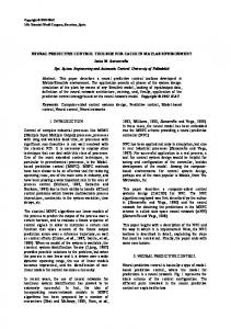
I. INTRODUCTION Nowadays, the road transportation system is becoming much more busy as more vehicles are manufactured and more journeys are made. To make the transport and mobility more intelligent and efficient, autonomous (self-driving) vehicles are considered as the promising solutions. With significant achievements in external sensing, motion planing and vehicle control, innovations around autonomous vehicle can assist the vehicles run independently in predefined scenarios well [1]. Generally, the system architectures in autonomous vehicles consist of three main processing modules, see Fig. 1 as an illustration [2]. The data provided by the sensors and digital maps are conducted in the perception and localization module to present representative features of the driving situation. The motion planning module aims to generate the appropriate decision-making strategy and derive an optimal trajectory

This work was supported by Foundation of State Key Laboratory of Automotive Simulation and Control (Grant No.20171108). (Corresponding author: Dongpu Cao) Teng Liu is with the State Key Laboratory of Automotive Simulation and Control, Jilin University, China, and He is also with the Vehicle Intelligence Pioneers Inc., Qingdao Shandong 266109, China. (email: tengliu17 @gmail.com). Hong Wang is with Mechanical and Mechatronics Engineering Department, Waterloo University, N2L 3G1, Canada (email: [email protected]) Li Li is with Faculty of Department of Automation, Tsinghua University, China. (email: [email protected]). D. Cao is with the Center for Automotive Engineering, University of Waterloo, Canada. (email: [email protected]). Fei-Yue Wang is with the State Key Laboratory of Management and Control for Complex Systems, Institute of Automation, Chinese Academy of Sciences, Beijing 100190 China (e-mail: [email protected]).

Lateral Trajectory Control Longitudinal Command

Control Actuator Fig. 1. System architecture of the general autonomous vehicle [2].

control actions to handle the acceletation and steering in order to maintain the existing trajectory [3]. The decision-making and path planning strategy is the key technology in the autonomous vehicle. Several techniques have been proposed to discuss the trajectory generation step. For example, a data-driven control framework named learning-by -demonstration is presented to train the controller from historical driving data to operate the vehicle as a human driver. Specifically, artificial neural networks (ANN) [4] and inverse optimal control [5] have been implemented to reproduce human driving behavior in a self-driving vehicle. However, the vehicle cannot run smoothly when the current driving situation is absent in the historical dataset. As alternative, model predictive control (MPC) [6] is used to predict the driver behavior and enforces multiple constraints in the cost function. The precision of the driving condition prediction decides the control performance of the MPC approach [7]. The big difference between the automated driving and human driver is to ensure the safety and comfort of its passengers. How to create a feasible, safe and comfortable reference trajectory is still a serious challenge. In this work, a learning-based predictive control framework is developed for self-driving hybrid electric vehicle (HEV). The proposed approach is bi-level. The higher-level is a human-like driver model, which can generate the

acceleration command to replicate a human driver’s demo nstration. The lower-level is a reinforcement learning (RL)-based controller, which is able to improve the energy efficiency of the autonomous HEV. The proposed framework is validated for the longitudinal control in the car following model. Results show that the proposed method can reproduce human driver’s driving style and improve fuel economy. The contributions of this work contain two aspects. First is adaptive to the current driving situation that is absent in the training dataset. The induced matrix norm (IMN) is presented to compare the difference between the current and historical driving data and to expand the training dataset. Second is combining the trajectory generation step with the energy efficiency improvement for the autonomous HEV. Based on the reference trajectory obtained from the higher-level, the RL-based controller enforces the battery and fuel consumption constraints in the cost function to promote the fuel economy. The rest of this paper is organized as follows. The higher-level driver modeling method is introduced in Section II. Section III describes the lower-level RL controller of HEV powertrain. Simulation results are presented in Section IV and Section V concludes the paper.

the hidden mode at time instant t and ot = [ωt, at] is the observation vector at time t, including the driving situation and acceleration. For HMC, the hidden modes are correlated with the observation via probability distribution as follow t

P(m1:t , 1:t , a1:t ) = P(m1 )  [ P(mk mk −1 )  P(k , ak mk )] (1) k =2

where the transition probability P(ωk, ak | mk) is assumed to comply with Gaussian distribution. Specially, the parameters of the HMC model consist of the initial distribution P(m1), the total hidden modes M, the transition probabilities πij means the transition from i-th mode to the j-th mode, and the covariance and mean matrix of the Gaussian distribution. Expectation-maximization algorithm and Bayesian information criterion are utilized to learn these parameters from the historical driving data [8]. C. Calculation for Current Acceleration Gaussian mixture regression is used to calculate the current acceleration via giving the driving situation sequence ω1:t as follow [3]

at = E[at 1 ,...t ]

II. THE HIGHER-LEVEL: DRIVER MODELING The human-like driver model in the higher-level is illustrated in this section. First, the parameters in the car following model are defined. Then, the methods for training the driver model are introduced. Finally, the prediction process of the future acceleration is described. A. Car Following Modeling In the car following model, the objective autonomous HEV is named as target vehicle and the autonomous HEV ahead is called as the front vehicle. Define δt=[dt, vt] is the state of the target vehicle at time instant t, where dt and vt are the longitudinal position and velocity, respectively. Similarly, δft=[dft, vft] is the state of the front vehicle at time instant t. The driving situation at time instant t is represented by the features ωt=[drt, vrt, vt], where drt= dft－d is the relative distance and vrt= vft－v is the relative velocity. In the higher-level, the driver model aims to generate an acceleration sequence At = [at, …, at+N-1] to guide the operation of the target vehicle. N=T/△t denotes the total time steps, T is the time interval for prediction and △t is the sampling time for driver model. Based on this acceleration sequence, the RL-based controller is applied to derive the power split control policy for the autonomous HEV in the lower-level. B. Training for Driver Model Based on the historical driving data ω1:t = [ω1, …, ωt], the goal of the driver model is to predict acceleration sequences that are close to the human driver’s real operations. For real driving data, the human driver’s control strategies are modeled as hidden Markov Chain (HMC), where mt∈{1,…M} is

M

−1  =   k ,t  [ ka + ak (  k ) (t − k )]

(2)

k =1

where

 k    k a  k k =  a  , k =  a aa   k   k k  αk, t denotes the mixing coefficient and is calculated as the probability of being in mode mt=k by [3]

 k ,t

( iM=1 i ,t −1   ik )  P(t k ,  k ) (3) = M M   j =1[( i =1 i ,t −1   ij )  P(t  j ,  j )]

D. Prediction for Future Acceleration As the current driving situation ωt=[drt, vrt, vt], the current acceleration at and the discretization time △t are known prior, the future driving situation can be computed by assuming the velocity of the front vehicle is constant as

1  r r r 2 d t +1 = d t + vt t − 2 at ( t )  r r vt +1 = vt − at t v = v + a t t t  t +1 

(4)

Compactly, the Eq. (4) can be reformulated as the state-space equation by

t +1 = Ct + Dat  at = E[at 1 ,...t ]

(5)

Finally, the future acceleration sequence over the prediction horizon T is able to be derived by iterating the following expression

t +1 = Ct + Datp  p p at +1 = E[at +1 1 ,...t +1 ]  p p  At = [at ,..., at + N −1 ]

(6)

III. THE LOWER-LEVEL: RL CONTROLLER The RL-based fuel saving controller is introduced in this section. First, the transition probability matrix (TPM) of the acceleration sequence is computed. Then, the induced matrix norm (IMN) is proposed to evaluate the difference between the historical and current acceleration data. Furthermore, the cost function of the energy efficiency improvement problem for the autonomous HEV is formulated. Finally, RL method framework is constructed and Q-learning algorithm is utilized to search the optimal control policy. A. TPM for Acceleration Sequence The acceleration sequence is treated as a finite Markov chain (MC) and its transition probability is calculated by the statistical method as

N ik , j   pik , j = P ( a j ai , vk ) = N  ik  M  N = N i, j = 1, 2,... N ik , j  ik  j =1

B. Induced Matrix Norm When the historical driving dataset does not contain the current driving situation, the driver model in the higher-level cannot generate efficient acceleration commands to guide the operation of the autonomous HEV. Hence, induced matrix norm (IMN) is introduced to quantify the difference of TPM for the historical and current acceleration sequences as

xR N {0}

IMN ( P1 ||P2 )= P1 − P2 2 = max i ( P1 − P2 ) 1i  N

= max i (( P1 − P2 )T ( P1 − P2 ))

( P1 − P2 ) x (8) x

where sup depicts the supremum of a scalar, and x is a N×1 dimension non-zero vector. The second-order norm in Eq. (8)

(9)

1i  N

where PT denotes the transpose of matrix P, and λi(P) represents the eigenvalue of matrix P for i=1, …, N. Note that the closer the IMN is to zero, the more similar the TPM P1 is to P2. C. Cost Function for Energy Efficiency The objective of energy efficiency improvement for the autonomous HEV is searching the optimal control under the constraints of components aim to improve the fuel economy while maintaining the charge sustaining constraint over the finite prediction horizon as T  2  J =  [m f (t ) +  (  SOC ) ]dt 0  (10)   SOC (t ) − SOCref SOC (t )  SOCref  =  SOC  0 SOC (t )  SOCref  

where mf is the fuel consumption rate, SOC is the state of charge of battery, θ is a large positive weighting factor to restrict the terminal value of SOC, and SOCref is a pre-defined factor to satisfy the charge-sustaining constraints [9]. The parameters of main components for the autonomous HEV are listed in Table I. TABLE I PARAMETERS OF MAIN COMPONENTS IN AUTONOMOUS HEV

(7)

where Nik, j is the number of times for the transition from ai to aj has occurred at vehicle speed vk, Nik is the total transition counts initiated from ai at vehicle speed vk, k is the discrete time step, and N is the amount of discrete acceleration index. The TPM P of the acceleration sequence is filled with elements pik, j. The TPMs for the historical and current acceleration sequences are denoted as P1 and P2, respectively.

IMN ( P1||P2 )= P1 − P2 2 = sup

can be reformulated as the following expression for convenient calculation

Symbol

Items

Values

Mv

Curb weight

800 kg

A

Fronted area

1.2 m2

Cd

Aerodynamic coefficient

0.60

ηT

Transmission axle efficiency

0.85

ηmot

Efficiency of Traction motor

0.93

f

Coefficient of Rolling resistance

0.0051

R

Tire radius

0.508 m

ρa

Air density

1.293 kg/m3

g

Gravitational constant

9.81 m/s2

D. RL Method The TPMs of predictive acceleration sequences and vehicle parameters are the inputs of RL approach for optimal control calculation. In the RL construction, a learning agent interacts with a stochastic environment. The interaction is modeled as quintuple (S, A, P, R, β), wherein S and A are the state variables and control actions set, P represents the TPM for power request, R denotes the reward gather, and β∈(0, 1) means a discount factor.

The control policy ψ is the distribution of the control commands a. The finite expected discounted and accumulated rewards is summarized as the optimal value function as T

V ( s ) = min E (   r ( s, a )) *

t



(11)

t =0

To deduce the optimal control action at each time instant, Eq. (11) is reformulated recursively as

V * ( s ) = min( r ( s, a ) +   psa ,sV * ( s)) s  S (12) a

sS

where psa,s´denotes the transition probability from state s to state s´using action a. The optimal control policy is determined based on the optimal value function in Eq. (12)

 * ( s ) = arg min( r ( s, a ) +   psa ,sV * ( s)) a

discussed. Furthermore, the control effectiveness of the RL-based fuel saving strategy is illustrated. A. Validation for Driver Model The driver model described in Section II is employed to predict the acceleration sequence in different driving situations. The mean square error (MSE) is used to quantify the differences between the predicted and actual acceleration sequences. Fig. 2 and Fig. 3 illustrate two realistic acceleration sequences and their prediction values for two driving situations A and B. For Fig. 2, the current driving style of the autonomous HEV is assumed to be existent in the historical driving dataset. Oppositely, the current driving style in Fig. 3 is absent in the training data.

(13)

sS

Furthermore, the action value function and its corresponding optimal measure are described as follow [10]

Q ( s, a ) = r ( s, a ) +   psa ,sQ ( s, a )  sS (14)  * Q ( s, a ). Q ( s, a ) = r ( s, a ) +   psa ,s min a  sS Finally, the updated criterion for the action value function in the Q-learning algorithm is indicated by

Q ( s, a )  Q ( s, a ) +  ( r ( s, a ) +  min Q ( s , a ) − Q ( s, a )) (15) a

where τ∈[0, 1] is a decaying factor in Q-learning algorithm. Table II describes the pseudo-code of Q-learning algorithm. The discount factor β is taken as 0.95, the decaying factor τ is related with the time step k and taken as 1 / k + 1 to accelerate the convergence rate, the iterative times K is 10000, and the sampling time is 1 second. The effectiveness of the proposed learning-based predictive control technique is validated in Section IV. TABLE II PSEUDO-CODE OF THE Q-LEARNING ALGORITHM

Fig. 2. The predicted and actual acceleration sequences for situation A.

It is apparent that the predicted value of the acceleration sequence is very close to the actual value for driving situation A in Fig. 2. This indicates that the driver model can achieve excellent accuracy when the historical driving dataset traverses the current driving situation A in advance. However, when the current driving situation B is missing in the training data, the driver model cannot give accurate guidance for the autonomous HEV operation, see Fig. 3 as an illustration. The MSE in Fig. 2 equals to 1.57, which is better than that in Fig. 3 (MSE=4.43) in the predicted availability.

Algorithm: Q-learning Algorithm 1. Extract Q(s, a) from training and initialize iteration number Nit 2. Repeat time instant k=1, 2, 3… 3. Based on Q(s, .), choose action a (ε-greedy policy) 4. Executing action a and observe r, s' 5. Define a*=arg mina Q(s', a) 6. Q(s, a)←Q(s, a)+ μ(r(s, a)+ γmin a' Q(s', a')-Q(s, a)) 7. s←s' 8. until s is terminal

IV. SIMULATION RESULTS AND DISCUSSION The presented learning-based predictive control framework is evaluated in this section. First, the performance of the driver model for acceleration sequence prediction is

Fig. 3. The predicted and actual acceleration sequences for situation B.

B. Validation for RL Controller Based on the historical and current acceleration sequences, the computational process of the TPM depicted in Section

III-A is applied to calculate the TPMs of acceleration in driving situations A and B. IMN is utilized to quantify the difference between these two sequences. As the IMN value exceeds the pre-defined threshold value, which means the current driving situation is different from the historical driving data, and thus the predicted acceleration is not precise. Conversely, the small IMN value implies that the predicted acceleration sequence learned from the historical data can be accurate. Fig. 4 and Fig. 5 show the IMN values at different vehicle velocity levels corresponding to the two driving situations in Fig. 2 and Fig. 3, respectively. These two figures indicate that the times for the IMN value exceeds the pre-defined threshold value are different. To handle the condition that the current driving situation B is absent in the historical driving data, this driving data will be added into the training dataset when the IMN value exceeds the threshold value. By doing this, the historical driving dataset is able to predict the human driver’s behavior accurately in the same driving situation.

data based on IMN value, the predictive RL is also superior to the common RL.

Fig. 6. SOC trajectories in common and predictive RL for two situations.

Fig. 4. IMN values at different velocity levels for driving situation A.

Fig. 5. IMN values at different velocity levels for driving situation B.

The exact TPM of the future acceleration sequence is further used to derive the fuel saving control using RL technique. Fig. 6 depicts the SOC trajectories for the common RL without the prediction acceleration information and the predictive RL with that information. It is noticed that the SOC trajectories are dramatically different in these two driving situations. This is caused by the adaptive controls that are decided by the TPM of the future acceleration sequence. For driving situation B, due to the expanded process of driving

Also, Fig. 7 illustrates the working area of the engine in multiple fuel saving controls. The engine working area under the proposed predictive RL control locates in the lower fuel consumption region more frequently, compared to the common RL control. This means that the predictive RL method can achieve higher fuel economy compared with the common RL technique.

Fig. 7. Engine working points in common and predictive RL for two situations.

Table III describes the fuel consumption after SOC correction in these two methods for driving situations A and B. It is apparent that the fuel consumption under the predictive RL control is lower than that of the common RL control. The predicted acceleration sequence makes RL-based control adapt to the future driving situation more compatibly, which contributes to the higher fuel economy. TABLE III THE FUEL CONSUMPTION IN DIFFERENT CONTROLS FOR TWO SITUATIONS

Driving Situation Driving situation A

Driving situation B a

Algorithms

Fuel Consu. (g)

Decrease (%)

Common RL

776.23

―

Predictive RL

676.13

12.9

Common RL

748.61

―

Predictive RL

674.51

9.9

A 2.7 GHz microprocessor with 3.8 GB RAM was used.

V. CONCLUSION In this paper, we seek energy efficiency improvement for the autonomous HEV by proposing a bi-level learning-based predictive control framework. First, the higher-level models the human driver’s behavior via using the hidden Markov Chain and Gaussian distribution. The lower-level is a reinforcement learning-based controller, which aims to improve the energy efficiency of the autonomous HEV. The proposed framework is validated for the longitudinal control in the car following model. Simulation results prove that the presented driver model can accurately predict the future acceleration sequence by using the induced matrix norm. Tests also prove that the predictive RL control based on the TPM of future acceleration sequence can achieve higher fuel economy compared with common RL control. The future work includes applying the proposed control framework into the real-time application and formulating the driver model using RL method to handle the lane-changing decision. REFERENCES [1]

X. Meng, S. Roberts, and Y. Cui, “Required navigation performance

for connected and autonomous vehicles: where are we now and where are we going?” Transportation Planning and Technology., vol. 41, no.1, pp. 104–118, 2018. [2] J. Ziegler, P. Bender, and M. Schreiber, “Making Bertha drive—An autonomous journey on a historic route,” IEEE Intell. Transportation Syst. Mag., vol. 6, no. 2, pp. 8–20, 2014. [3] S. Lefevre, A. Garvalho, and F. Borrelli, “A learning-based framework for velocity control in autonomous driving,” IEEE Intell. Autom. Sci. Eng., vol. 13, no. 1, pp. 32-42, 2016. [4] D. A. Pomerleau, “Alvinn: An autonomous land vehicle in a neural network,” in Proc. Adv. Neural Inf. Process. Syst., 1989, pp. 305–313. [5] S. Levine and V. Koltun, “Continuous inverse optimal control with locally optimal examples,” in Proc. Int. Conf. Mach. Learning, 2012, pp. 41–48. [6] A. Carvalho, Y. Gao, S. Lefèvre, and F. Borrelli, “Stochastic predictive control of autonomous vehicles in uncertain environments,” in Proc. 12th Int. Symp. Adv. Veh. Control, 2014. [7] P. Liu, U. Ozguner, and Y. Zhang, “Distributed MPC for cooperative highway driving and energy economy validation via microscopic simulations,” Transportation Research Part C, vol. 77, pp. 80-95, 2017. [8] S. Calinon, F. D'halluin, E. Sauser, D. Caldwell, and A. Billard, “Learning and reproduction of gestures by imitation,” IEEE Robot. Autom. Mag., vol. 17, no. 2, pp. 44–54, 2010. [9] Y. Zou, T. Liu, D. X. Liu and F. C. Sun, “Reinforcement learning-based real-time energy management for a hybrid tracked vehicle,” Appl Energy, vol. 171, pp. 372-382, 2016. [10] L. Kaelbing, M. Littman, and A. Moore, “Reinforcement learning: A Survey,” Journal of Artificial Intelligence Research, vol. 4, pp. 237-285, 1996.