Generalized Predictive Control and Neural Generalized Predictive ...

Leonardo Journal of Sciences

Issue 13, July-December 2008

ISSN 1583-0233

p. 133-152

Generalized Predictive Control and Neural Generalized Predictive Control Sadhana CHIDRAWAR1, Balasaheb PATRE1 Asst. Prof, MGM’s College of Engineering, Nanded (MS) 431 602 Professor, S.G.G.S. Institute of Engineering And Technology, Nanded (MS) 431 606 E-mail(s): [email protected]. [email protected] Abstract As Model Predictive Control (MPC) relies on the predictive Control using a multilayer feed forward network as the plants linear model is presented. In using Newton-Raphson as the optimization algorithm, the number of iterations needed for convergence is significantly reduced from other techniques. This paper presents a detailed derivation of the Generalized Predictive Control and Neural Generalized Predictive Control with NewtonRaphson as minimization algorithm. Taking three separate systems, performances of the system has been tested. Simulation results show the effect of neural network on Generalized Predictive Control. The performance comparison of this three system configurations has been given in terms of ISE and IAE. Keywords Neural network; Model predictive control; GPC; NGPC.

Introduction In recent years, the requirements for the quality of automatic control in the process industries increased significantly due to the increased complexity of the plants and sharper specifications of product quality. At the same time, the available computing power increased to a very high level. As a result, computer models that are computationally expensive became

http://ljs.academicdirect.org

133

Generalized Predictive Control and Neural Generalized Predictive Control Sadhana CHIDRAWAR, Balasaheb PATRE

applicable even to rather complex problems. Intelligent and model based control techniques were developed to obtain tighter control for such applications. In recent years, incorporation of neural networks as intelligent control techniques, to adaptive control system design has been claimed to be a new method for the control of systems with significant nonlinearities. Those neural network based control systems so far developed are generally classified as indirect or direct control methods. Model predictive control (MPC) has found a wide range of applications in the process, chemical, food processing and paper industries. Some of the most popular MPC algorithms that found a wide acceptance in industry are Dynamic Matrix Control (DMC), Model Algorithmic Control (MAC), Predictive Functional Control (PFC), Extended Prediction Self Adaptive Control (EPSAC), Extended Horizon Adaptive Control (EHAC) and Generalized Predictive Control (GPC). In this work, among these number of MPC algorithms GPC is studied in detail.

Generalized Predictive Control (GPC) The GPC method was proposed by Clarke et al [1] and has become one of the most popular MPC methods both in industry and academia. It has been successfully implemented in many industrial applications, showing good performance and a certain degree of robustness. The basic idea of GPC is to calculate a sequence of future control signals in such a way that it minimizes a multistage cost function defined over a prediction horizon. The index to be optimized is the expectation of a quadratic function measuring the distance between the predicted system output and some reference sequence over the horizon plus a quadratic function measuring the control effort. Generalized Predictive Control has many ideas in common with the other predictive controllers since it is based upon the same concepts but it also has some differences. As will be seen later, it provides an analytical solution (in the absence of constraints), it can deal with unstable and non-minimum phase plants and incorporates the concept of control horizon as well as the consideration of weighting of control increments in the cost function. The general set of choices available for GPC leads to a greater variety of control objective compared to other approaches, some of which can be considered as subsets or limiting cases of GPC.

134



ISSN 1583-0233

p. 133-152

The GPC scheme can be seen in Fig. 1. It consists of the plant to be controlled, a reference model that specifies the desired performance of the plant, a linear model of the plant, and the Cost Function Minimization (CFM) algorithm that determines the input needed to produce the plant’s desired performance. The GPC algorithm consists of the CFM block. The GPC system starts with the input signal, r(t), which is presented to the reference model. This model produces a tracking reference signal, w (t) that is used as an input to the CFM block. The CFM algorithm produces an output, which is used as an input to the plant. Between samples, the CFM algorithm uses this model to calculate the next control input, u (t+1), from predictions of the response from the plant’s model. Once the cost function is minimized, this input is passed to the plant. This algorithm is outlined below.

GPC

w(t)

Cost Function Minimization (CFM) Algorithm

y(t) Process

Linear Model of Process

Figure 1. Basic Structure of GPC Formulation of Generalized Predictive Control Most single-input single-output (SISO) plants, when considering operation around particular set points and after linearization, can be described by Equation (1) [2]. A( z −1 ) y (t ) = z − d B ( z −1 )u (t − 1) + C ( z −1 )e(t )

(1)

where u (t ) and y (t ) are the control and output sequence of the plant and e(t ) is a zero mean white noise. A , B And C are the following polynomials in the backward shift operator z −1 :

A( z −1 ) = 1 + a1 z −1 + a2 z −2 + ...... + ana z − na

B( z −1 ) = b0 + b1 z −1 + b2 z −2 + ...... + bnb z − nb C ( z −1 ) = 1 + c1 z −1 + c2 z −2 + ...... + cnc z − nc

135

Generalized Predictive Control and Neural Generalized Predictive Control Sadhana CHIDRAWAR, Balasaheb PATRE

Where, d is the dead time of the system. This model is known as a Controller AutoRegressive Moving-Average (CARIMA) model. It has been argued that for many industrial applications in which disturbances are non-stationary an integrated CARMA (CARIMA) model is more appropriate. A CARIMA model is given by Equation (2): A( z −1 ) y (t ) = z − d B ( z −1 )u (t − 1) + C ( z −1 )

e(t ) Δ

(2)

Δ = 1 − z −1

with

For simplicity, C polynomial in Equation (2) is chosen to be 1. Notice that if C −1 can be truncated it can be absorbed into A and B .

Cost Function

GPC algorithm consists of applying a control sequence that minimizes a multistage cost function of the form given in Equation (3)

J ( N1 , N 2 , Nu ) =

λ ( j )[ Δu (t + j −1)] ∑ δ ( j )[ yˆ (t + j |t ) − w(t + j )] + ∑ j= j= N2

2

N1

Nu

2

(3)

1

where yˆ (t + j | t ) is an optimum j-step ahead prediction of the system output on data up to time

k, N1 and N 2 are the minimum and maximum costing horizons, Nu control horizon, δ ( j ) and λ ( j ) are weighing sequences and w(t + j ) is the future reference trajectory, which can considered to be constant. The objective of predictive control is to compute the future control sequence u (t ) ,

u (t + 1) ,… u (t + Nu ) in such a way that the future plant output y (t + j ) is driven close to w(t + j ) . This is accomplished by minimizing J ( N1 , N 2 , Nu ) .

Cost Function Minimization Algorithm

In order to optimize the cost function the optimal prediction of y (t + j ) for j ≥ N1 and j ≤ N 2 is required. To compute the predicted output, consider the following Diophantine Equation (4): 1 = E j ( z −1 ) A% ( z −1 ) + z − j Fj ( z −1 ) With A% ( z −1 ) = ΔA( z −1 )

(4)

The polynomials E j and Fj are uniquely defined with degrees j − 1 and na respectively. They can be obtained dividing 1 by A% ( z −1 ) until the remainder can be factorized

136



ISSN 1583-0233

p. 133-152

as z − j Fj ( z −1 ) . The quotient of the division is the polynomial E j ( z −1 ) . An example demonstrating calculation of Ej and Fj coefficients in Diophantine Equation is shown in Example 1 below:

Example 1: Diophantine Equation Demonstration Example

Introduction to Neural Generalized Predictive Control

The ability of the GPC to make accurate predictions can be enhanced if a neural network is used to learn the dynamics of the plant instead of standard nonlinear modeling techniques. [3] The selection of the minimization algorithm affects the computational efficiency of the algorithm. Explicit solution for it can be obtained if the criterion is quadratic, the model is linear and there are no constraints; otherwise an iterative optimization method has to be used. In this project work Newton-Raphson method is used as the optimization

137

Generalized Predictive Control and Neural Generalized Predictive Control

Sadhana CHIDRAWAR, Balasaheb PATRE

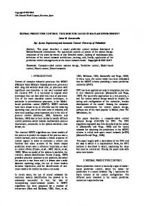
algorithm. The main cost of the Newton-Raphson algorithm is in the calculation of the Hessian, but even with this overhead the low iteration numbers make Newton-Raphson a faster algorithm for real-time control [4]. The Neural Generalized Predictive Control (NGPC) system can be seen in Fig. 2. It consists of four components, the plant to be controlled, a reference model that specifies the desired performance of the plant, a neural network that models the plant, and the Cost Function Minimization (CFM) algorithm that determines the input needed to produce the plant’s desired performance. The NGPC algorithm consists of the CFM block and the neural net block.

ym(n) ym(n) Cost Function Minimization (CFM)

u(n)

s

y(n)

Plant s z

-1

Neural Plant Model

∧ yn (t + k⏐t)

NGPC Algorithm Figure 2. Block Diagram of NGPC System

The NGPC system starts with the input signal, r(n), which is presented to the reference model. This model produces a tracking reference signal, ym(n), that is used as an input to the CFM block. The CFM algorithm produces an output that is either used as an input to the plant or the plant’s model. The double pole double throw switch, S, is set to the plant when the CFM algorithm has solved for the best input, u(n), that will minimize a specified cost function. Between samples, the switch is set to the plant’s model where the CFM algorithm uses this model to calculate the next control input, u(n+1), from predictions of the response from the plant’s model. Once the cost function is minimized, this input is passed to the plant. This algorithm is outlined below. The computational performance of a GPC implementation is largely based on the minimization algorithm chosen for the CFM block. The selection of a minimization method can be based on several criteria such as: number of iterations to a solution, computational costs and accuracy of the solution. In general these approaches are iteration intensive thus

138



ISSN 1583-0233

p. 133-152

making real-time control difficult. In this work Newton-Raphson as an optimization technique is used. Newton-Raphson is a quadratic ally converging. The improved convergence rate of Newton-Raphson is computationally costly, but is justified by the high convergence rate of Newton-Raphson. The quality of the plant’s model affects the accuracy of a prediction. A reasonable model of the plant is required to implement GPC. With a linear plant there are tools and techniques available to make modeling easier, but when the plant is nonlinear this task is more difficult. Currently there are two techniques used to model nonlinear plants. One is to linearize the plant about a set of operating points. If the plant is highly nonlinear the set of operating points can be very large. The second technique involves developing a nonlinear model which depends on making assumptions about the dynamics of the nonlinear plant. If these assumptions are incorrect the accuracy of the model will be reduced. Models using neural networks have been shown to have the capability to capture nonlinear dynamics. For nonlinear plants, the ability of the GPC to make accurate predictions can be enhanced if a neural network is used to learn the dynamics of the plant instead of standard modeling techniques. Improved predictions affect rise time, over-shoot, and the energy content of the control signal.

Formulation of NGPC Cost Function

As mentioned earlier, the NGPC algorithm [4] is based on minimizing a cost function over a finite prediction horizon. The cost function of interest to this application is J ( N1 , N 2 , Nu ) =

∑ δ ( j )[ yˆ j= N2

N1

(t + j |t ) − w(t + j ) n

]

2

Nu

[

+ ∑ λ ( j ) Δu (t + j −1) j =1

]

2

(5)

N1 = Minimum Costing Prediction Horizon N2 = Maximum Costing Prediction Horizon Nu= Length of Control Horizon

∧ y (t + k⏐t ) = Predicted Output from Neural; Network

u (t + k⏐) t = Manipulated Input w(t + k ) = Reference Trajectory δ and λ = Weighing Factor

139



This cost function minimizes not only the mean squared error between the reference signal and the plant’s model, but also the weighted squared rate of change of the control input with it’s constraints. When this cost function is minimized, a control input that meets the constraints is generated that allows the plant to track the reference trajectory within some tolerance. There are four tuning parameters in the cost function, N1, N2, Nu, and λ. The predictions of the plant will run from N1 to N2 future time steps. The bound on the control horizon is Nu. The only constraint on the values of Nu and N1 is that these bounds must be less than or equal to N2. The second summation contains a weighting factor, λ that is introduced to control the balance between the first two summations. The weighting factor acts as a damper on the predicted u (n+1).

Cost Function Minimization Algorithm

The objective of the CFM algorithm is to minimize J in Equation (6) with respect to [u(n+l), u(n+2), ..., u(n+Nu)]T, denoted U. This is accomplished by setting the Jacobian of Equation (5) to zero and solving for U. With Newton-Rhapson used as the CFM algorithm, J is minimized iteratively to determine the best U. An iterative process yields intermediate values for J denoted J(k). For each iteration of J(k) an intermediate control input vector is also generated and is denoted as in Equation (6): ⎡ u (t + 1) ⎤ ⎢ u (t + 2) ⎥ ⎢ ⎥ Δ ⎢ ⎥ . U (k ) = ⎢ ⎥ . ⎢ ⎥ ⎢ ⎥ . ⎢ ⎥ ⎢⎣u (t + N u ) ⎥⎦

k=1,……Nu

(6)

Newton-Raphson method is one of the most widely used of all root-locating formula. If the initial guess at the root is xi, a tangent can be extended from the point [xi, f(xi)]. The point where this tangent crosses the x-axis usually represents an improved estimate of the root. So the first derivative at x on rearranging can be given as: x(i +1) = x( i ) − Using this Newton-Raphson update rule, U(k+1) is given by Equation (7)

140

f ( xi ) f ' ( xi )



ISSN 1583-0233

p. 133-152 −1

Where

⎛ ∂2 J ⎞ ∂J U (k + 1) = U (k ) − ⎜ (k ) ⎟ (k ) ' 2 ⎝ ∂U ⎠ ∂U ∂J f ( x) = ∂U

(7)

And the Jacobian is denoted as in Equation (8) ∂J ⎡ ⎤ ⎢ ∂u (t + 1) ⎥ ⎢ ⎥ . ⎢ ⎥ ∂J ⎢ ⎥ . (k ) ≡ ⎢ ⎥ ∂U ⎢ ⎥ . ⎢ ⎥ ∂J ⎢ ⎥ ⎢⎣ ∂u (t + N u ) ⎥⎦ And the Hessian as in Equation (9)

(8)

⎡ ∂2 J ⎢ ∂u (t + 1) 2 ⎢ ⎢ . ∂2 J ≡ k ( ) ⎢. 2 . ∂U ⎢ ⎢ ∂2 J ⎢ ⎣⎢ ∂u (t + N u )∂uk (t + 1)

⎤ ∂2 J ⎥ ∂u (t + 1)∂u (t + N u ) ⎥ ⎥ . . . ⎥ . . . ⎥ 2 ⎥ ∂ J ⎥ . . ∂u (t + N u )2 ⎦⎥ . .

(9)

Each element of the Jacobianis calculated by partially differentiating Equation (8) with respect to vector U. ∧

Nu N2 ∂Δu ( t + j ) ∂J ⎡∧ ⎤ ∂ yn ( t + j ) = 2 ∑ δ ( j ) ⎢ yn ( t + j ) − w(t + j ) ⎥ + 2∑ λ ( j ) ⎡⎣ Δu ( t + j ) ⎤⎦ (10) ∂u ( t + h ) ∂u ( t + h ) ⎣ ⎦ ∂u ( t + h ) j = N1 j =1

Where, h = 1,...., N u Once again Equation (10) is partially differentiated with respect to vector U to get each element of the Hessian. ^ ^ ^ ⎧ ⎫ N2 ^ ∂2 y (t + j ) ∂ + ∂ y t j y t + j)⎪ ( ( ) ∂2 J ⎪ ⎡ ⎤ = 2 ∑ δ ( j) ⎨ ⎢ y ( t + j ) − w ( t + j ) ⎥⎦ − ∂u ( t + m ) ∂u ( t + h ) ⎬ ∂u (t + m)∂u (t + h) j = N1 ⎪⎩ ∂u (t + m)∂u (t + h) ⎣ ⎪⎭ N2 ∂ 2 Δn ( t + j ) ⎪⎫ ⎪⎧ ∂Δn ( t + j ) ∂Δn ( t + j ) +2 ∑ λ ( j ) ⎨ + ⎬ j = N1 ⎩⎪ ∂u ( t + m ) ∂u ( t + h ) ∂u (t + m)∂u (t + h) ⎭⎪

(11)

141



The

mth , hth

elements

of

the

Hessian

matrix

in

Equation

(11)

are h = 1,....., N u and m = 1,....., N u . The last computation needed to evaluate U ( k + 1) is the calculation of the predicted ∧

output of the plant, y ( t + j ) , and it’s derivatives. The next sections define the equation of a multilayer feed forward neural network, and define the derivative equations of the neural network.

Neural Network Architecture

In NGPC the model of the plant is a neural network. This neural model is constructed and trained using MATLAB Neural Network System Identification Toolbox commands [5]. The output of trained neural network is used as the predicted output of the plant. This predicted output is used in the Cost Function Minimization Algorithm. If yn(t) is the neural

∧

network’s output then it is nothing but plant’s predicted output y n (t + k⏐t ) . The initial training of the neural network is typically done off-line before control is attempted. The block configuration for training a neural network to model the plant is shown in Fig. 3. The network and the plant receive the same input, u(t). The network has an additional input that either comes from the output of the plant, y(t), or the neural network’s, yn(t). The one that is selected depends on the plant and the application. This input assists the network with capturing the plant’s dynamics and stabilization of unstable systems. To train the network, its weights are adjusted such that a set of inputs produces the desired set of outputs. An error is formed between the responses of the network, yn(t), and the plant, y(t). This error is then used to update the weights of the network through gradient descent learning. In this work a Levenberg-Marquardt method is used as gradient descent learning algorithm for updating the weights. This is standard method for minimization of mean-square error criteria, due to its rapid convergence properties and robustness. This process is repeated until the error is reduced to an acceptable level. Since a neural network will be used to model the plant, the configuration of the network architecture should be considered. This implementation of NGPC adopts input/output models.

142



ISSN 1583-0233

p. 133-152

u(t)

y(t)

Plant s z

-1

Neural Plant yn (t) Model

-

+

e(t)

Figure 3. Block Diagram of Off-line Neural Network Training

The diagram below, Fig.4, depicts a multi-layer feed-forward neural network with a time-delayed structure. For this example, the inputs to this network consists of two external inputs, u(t) and two outputs y(t-1), with their corresponding delay nodes, u(t), u(t-1) and y(t1), y(t-2). The network has one hidden layer containing five hidden nodes that uses bi-polar sigmoidal activation output function. There is a single output node which uses a linear output function, of one for scaling the output. Input Hidden Layer Layer

Output Layer

Y(t-1) Y(t-2)

u(k)

U(t) U(t-1)

Figure 4. Neural Network Architecture

The equation for this network architecture is: hid

yn ( t ) = ∑ w j f j ( net ( t ) ) j =1

And nd

dd

j =1

j =1

net j ( t ) = ∑ w j ,i +1u ( t − i ) + ∑ w j ,nd +i +1 y ( t − i ) Where,

yn ( t )

(12)

is the output of the neural network

143



f j ( .)

is the output function for the j th node of the hidden layer

net j ( t )

is the activation level of the j th node’s output function

hid nd

is the number of hidden nodes in the hidden layer is the number of input nodes associated with u (.)

dd

is the number of input nodes associated with y (.)

wj

is the weight connecting the j th hidden node to the output node

w j ,i

is the weight connecting the i th hidden input node to the j th hidden

node y (t − i )

is the delayed output of the plant used as input to the network

u (t − i )

is the input to the network and its delays

This neural network is trained in offline condition with plants input/output data

Prediction Using Neural Network

The NGPC algorithm uses the output of the plant's model to predict the plant's dynamics to an arbitrary input from the current time, t, to some future time, t+k. This is accomplished by time shifting equations Equation (11) and (12), by k, resulting in Equation (13) and (14). hid

yn (t + k ) = ∑ w j f j ( net j ( t + k ) )

(13)

j =1

And min ( k , d d ) ⎪⎧u ( n + k − i ) , k − N u < i + ∑ w j ,nd +i +1 yn ( t + k − i ) net j ( t + k ) = ∑ w j ,i +1 ⎨ i =1 j =1 ⎪⎩ u ( n + N u ) , k − N u ≥ i hid

(

dd

(

+ ∑ w j ,nd +i +1 y ( t + k − i ) i = k +1

)

(14

)

The first summation of Equation (14) breaks the input into two parts represented by the conditional. The condition where k − N u < i handles the previous future values of the u up to u ( t + N u − 1) . The condition where k − N u > i sets the input from u ( t + N u ) to u ( t + k ) equal to u ( t + N u ) . The second condition will only occur if N 2 > N u . The next summation of Equation (14) handles the recursive part of prediction. This feeds back the network output, yn , for k or d d times, which ever is smaller. The last summation of Equation (14)

144



ISSN 1583-0233

p. 133-152

handles the previous values of y. The following section derives the derivatives of Equation (13) and (14) with respect to the input u ( t + h ) .

Neural Network Derivative Equations

To evaluate the Jacobian and the Hessian in Equation (8) and (9) the network’s first and second derivative with respect to the control input vector are needed.

Jacobian Element Calculation

The elements of the Jacobian are obtained by differentiating yn(t+k) in Equation (13) with respect to u(t+h) resulting in ∂yn ( t + k ) ∂u ( t + h )

hid

= ∑ wj j =1

∂f j ( net j ( t + k ) ) ∂u ( t + h )

(15)

Applying chain rule to ∂f j ( net j ( t + k ) ) ∂u ( t + h ) results in

∂f j ( net j ( t + k ) ) ∂u ( t + h )

=

∂f j ( net j ( t + k ) ) ∂net j ( t + k ) ∂net j ( t + k )

∂u ( t + h )

(16)

Where ∂f j ( net j ( t + k ) ) ∂net j ( t + k ) is the output function’s derivative which will become zero as we are using a linear (constant value) output activation function and

∂net j ( t + k )

nd ⎪⎧δ ( k − i, h ) , k − N u < i = ∑ w j ,i +1 ⎨ ∂u ( t + h ) i =0 ⎪⎩ δ ( N u , h ) , k − Nu ≥ i min( k , d d ) ∂yn ( t + k − i ) δ1 ( k − i − 1) + ∑ w j ,i + nd +1 ∂u ( t + h ) i =0

(17)

Note that in the last summation of Equation (17) the step function, δ, was introduced. This was added to point out that this summation evaluates to zero for k-i