Mar 19, 2018 - Burke, Edmund K, Matthew Hyde, Graham Kendall, and John Woodward ... In: Bell Labs Technical Journal ..... Sniady, Aleksander (2015).
Downloaded from orbit.dtu.dk on: Mar 19, 2018
Towards Signalling Maintenance Scheduling for European Railway Traffic Management System
M. Pour, Shahrzad; Rasmussen, Kourosh Marjani
Publication date: 2017 Document Version Publisher's PDF, also known as Version of record Link back to DTU Orbit
Citation (APA): M. Pour, S., & Rasmussen, K. M. (2017). Towards Signalling Maintenance Scheduling for European Railway Traffic Management System. Department of Management Engineering, Technical University of Denmark.
General rights Copyright and moral rights for the publications made accessible in the public portal are retained by the authors and/or other copyright owners and it is a condition of accessing publications that users recognise and abide by the legal requirements associated with these rights. • Users may download and print one copy of any publication from the public portal for the purpose of private study or research. • You may not further distribute the material or use it for any profit-making activity or commercial gain • You may freely distribute the URL identifying the publication in the public portal If you believe that this document breaches copyright please contact us providing details, and we will remove access to the work immediately and investigate your claim.
Towards Signalling Maintenance Scheduling for European Railway Traffic Management System
Shahrzad M. Pour Ph.D. Thesis
Technical University of Denmark Operations Research Group Department of Management Engineering Produktionstorvet Building 424 DK-2800 Kongens Lyngby Denmark Phone +(45) 45 25 48 00 www.man.dtu.dk Banedanmark Amerika Plads 15 DK-2100 Copenhagen Ø Denmark Phone +(45) 82 34 00 00 www.bane.dk Queen Mary University of London Operational Research Group Mile End Road London E1 4NS UK Phone +(44) 20 7882 5555 www.qmul.ac.uk
Shahrzad M. Pour Operations Research Group Department of Management Engineering Technical University of Denmark Supervisor Associate Professor Kourosh Marjani Rasmussen Division of Management Science Department of Management Engineering Technical University of Denmark External Supervisor Professor Edmund Kieran Burke Operational Research Group Queen Mary University of London
Assessment Committee Professor Harilaos Psaraftis Technical University of Denmark Denmark Professor Patrick De Causmaecker KU Leuven Belgium Associate Professor Ahmad Al Hanbali University of Twente The Netherlands
Preface
This Ph.D. thesis has been submitted to DTU Management Engineering at the Technical University of Denmark. The research has taken place during the period from 2013 to 2016 and fulfils the requirements for acquiring a Ph.D. in Engineering. The project has been co-funded by Banedanmark which is a state-owned company responsible for maintenance and traffic control of most of the Danish railway network. This work was supervised by Associate Professor Kourosh Marjani Rasmussen and Professor Edmund K. Burke from Queen Mary University of London. The focus of this thesis is to develop new maintenance plans for the Danish Railway system, which are useful for the current signalling system based on colourlight signalling and also for migrating towards the European Railway Traffic Management System (ERTMS). This thesis consists of two parts. The first part contains an overview of the research which introduces the thesis background, the signalling maintenance planning problem in Denmark, methods involved to address the thesis goals, literature review, and a concluding chapter. The second part is a collection of four academic papers developed during the Ph.D. research. 14-December-2016 Shahrzad M. Pour
ii
Table of Contents
Page Preface
i
Table of Contents
iii
List of Figures
vii
Summary
ix
Resumé
xi
Acknowledgements
xiii
List of Acronyms
I
xv
Research Overview
1 Introduction 1.1 Area of Concern . . . . . . . 1.2 Motivation . . . . . . . . . . 1.3 Purpose and Contributions . 1.3.1 Scheduling Framework 1.3.2 Scheduling Framework 1.4 Scope and Limitation . . . . 1.5 Thesis Organisation . . . . .
1 . . . . . . . . . . . . . . . . . . . . . . . . . . . . . . . . . . . . . . . . . . . . . . . . . . . . . . . . . for Shifting Towards ERTMS . . based on Colour-light signalling . . . . . . . . . . . . . . . . . . . . . . . . . . . . . . . . . . . . . . .
. . . . . . .
3 3 5 6 6 9 9 10
iv 2 Background 2.1 Railway Signalling System . . . . . . . 2.1.1 Evolution towards ERTMS . . 2.1.2 ERTMS . . . . . . . . . . . . . 2.1.3 Danish Signalling System . . . 2.2 Railway Maintenance . . . . . . . . . . 2.2.1 Maintenance Activities . . . . . 2.2.2 Railway Maintenance Planning 2.3 Signalling Maintenance in ERTMS . .
Table of Contents
. . . . . . . .
. . . . . . . .
. . . . . . . .
. . . . . . . .
. . . . . . . .
. . . . . . . .
13 13 15 18 19 22 22 23 24
3 Signalling Maintenance Planning in Denmark 3.1 Problem Addressed in ERTMS . . . . . . . . . . . . . . 3.1.1 Need for simultaneous presence of crew members 3.1.2 Need for clustering the maintenance region . . . 3.1.3 Abstract signalling maintenance problem model . 3.2 Problem Addressed in Colour-light Signalling . . . . . .
. . . . .
. . . . .
. . . . .
. . . . .
. . . . .
27 27 29 30 31 32
. . . . . . . . .
. . . . . . . . .
35 35 36 37 38 38 39 40 40 41
5 Literature Review 5.1 Maintenance Vehicle Routing and Scheduling Problem . . . . . 5.2 Vehicle Routing Problem with Time Window . . . . . . . . . . 5.2.1 VRPTW with Multiple Depot . . . . . . . . . . . . . . 5.2.2 VRP with Exact Operation Synchronisation Constraints 5.3 Constraint Programming . . . . . . . . . . . . . . . . . . . . . . 5.3.1 VRPs with Synchronisation constraints . . . . . . . . . 5.3.2 Scheduling problems . . . . . . . . . . . . . . . . . . . . 5.3.3 The railway system . . . . . . . . . . . . . . . . . . . . .
. . . . . . . .
43 43 47 47 50 52 52 53 55
6 Conclusion 6.1 Contributions and Novelties . . . . . . . . . . . . . . . . . . . . . 6.2 Future Work . . . . . . . . . . . . . . . . . . . . . . . . . . . . .
57 57 60
. . . . . . . .
. . . . . . . .
4 Methods Involved 4.1 Hyper-heuristic . . . . . . . . . . . . . . . 4.1.1 Classification . . . . . . . . . . . . 4.2 Constraint Programming . . . . . . . . . . 4.2.1 Constraint Propagation . . . . . . 4.2.2 Global Constraints . . . . . . . . . 4.2.3 Search Algorithms . . . . . . . . . 4.2.4 Constraint Satisfaction Problems . 4.2.5 Constraint Optimisation Problems 4.2.6 Google OR Tools . . . . . . . . . .
. . . . . . . .
. . . . . . . . .
. . . . . . . .
. . . . . . . . .
. . . . . . . .
. . . . . . . . .
. . . . . . . .
. . . . . . . . .
. . . . . . . .
. . . . . . . . .
. . . . . . . .
. . . . . . . . .
. . . . . . . .
. . . . . . . . .
. . . . . . . . .
. . . . . . . . .
. . . . . . . . .
. . . . . . . . .
v
II
Academic Papers
71
7 Clustering of Maintenance Tasks for the Danish Railway System 73 7.1 Introduction . . . . . . . . . . . . . . . . . . . . . . . . . . . . . . 74 7.2 Mathematical model . . . . . . . . . . . . . . . . . . . . . . . . . 75 7.3 Experimental results . . . . . . . . . . . . . . . . . . . . . . . . . 77 7.3.1 Experimental protocol . . . . . . . . . . . . . . . . . . . . 77 7.3.2 Benchmark instances . . . . . . . . . . . . . . . . . . . . . 77 7.3.3 Trade-off between the three problem criteria . . . . . . . . 79 7.3.4 Results and comparisons . . . . . . . . . . . . . . . . . . . 80 7.4 Conclusion . . . . . . . . . . . . . . . . . . . . . . . . . . . . . . 82 8 A Choice Function Hyper-heuristic Framework for the Allocation of Maintenance Tasks in Danish Railways 85 8.1 Introduction . . . . . . . . . . . . . . . . . . . . . . . . . . . . . . 86 8.2 Problem definition . . . . . . . . . . . . . . . . . . . . . . . . . . 89 8.2.1 Mathematical model . . . . . . . . . . . . . . . . . . . . . 89 8.2.2 Dataset . . . . . . . . . . . . . . . . . . . . . . . . . . . . 90 8.3 Proposed framework . . . . . . . . . . . . . . . . . . . . . . . . . 91 8.3.1 Initial solutions . . . . . . . . . . . . . . . . . . . . . . . . 92 8.3.2 Identifying outliers . . . . . . . . . . . . . . . . . . . . . . 93 8.3.3 Choice function heuristic selection . . . . . . . . . . . . . 94 8.3.4 Low-level heuristics . . . . . . . . . . . . . . . . . . . . . 96 8.3.5 Pseudocode for the proposed framework . . . . . . . . . . 98 8.4 Results and discussion . . . . . . . . . . . . . . . . . . . . . . . . 100 8.4.1 Quality of the initial solutions generated using different constructive heuristics . . . . . . . . . . . . . . . . . . . . 100 8.4.2 Results of CFHH using different initial solutions . . . . . 101 8.4.3 Comparison between CFHH and simple random hyperheuristic (SRHH) . . . . . . . . . . . . . . . . . . . . . . . 103 8.4.4 Detailed low-level heuristic performance . . . . . . . . . . 108 8.4.5 Trend of solution improvement during a run using CFHH 110 8.5 Conclusions . . . . . . . . . . . . . . . . . . . . . . . . . . . . . . 112 9 A Constructive Framework for the Preventive Signalling Maintenance Crew Scheduling Problem in the Danish Railway system 117 9.1 Introduction . . . . . . . . . . . . . . . . . . . . . . . . . . . . . . 118 9.2 Maintenance Planning in ERTMS . . . . . . . . . . . . . . . . . . 122 9.2.1 Requirement for clustering the maintenance region . . . . 123 9.2.2 MIP Formulation . . . . . . . . . . . . . . . . . . . . . . . 125 9.3 Proposed Solution Framework . . . . . . . . . . . . . . . . . . . . 127 9.3.1 First stage: The synchronisation set . . . . . . . . . . . . 128
vi
Table of Contents
9.4
9.5
9.6
9.3.2 Second stage: Clustering . . . . . . . . . . . 9.3.3 Third stage: Ordering clusters . . . . . . . 9.3.4 Fourth stage: Routing and scheduling . . . Routing and Scheduling Phase . . . . . . . . . . . 9.4.1 Terminology . . . . . . . . . . . . . . . . . 9.4.2 Route interdependency . . . . . . . . . . . . 9.4.3 The problem as a CSP . . . . . . . . . . . . Experimental results . . . . . . . . . . . . . . . . . 9.5.1 Test Case Description . . . . . . . . . . . . 9.5.2 Comparison with a commercial MIP solver 9.5.3 Main results . . . . . . . . . . . . . . . . . . 9.5.4 Clustering results . . . . . . . . . . . . . . . 9.5.5 Optimality gap . . . . . . . . . . . . . . . . Conclusion . . . . . . . . . . . . . . . . . . . . . .
. . . . . . . . . . . . . .
. . . . . . . . . . . . . .
. . . . . . . . . . . . . .
. . . . . . . . . . . . . .
. . . . . . . . . . . . . .
. . . . . . . . . . . . . .
. . . . . . . . . . . . . .
. . . . . . . . . . . . . .
129 130 131 132 132 132 133 142 142 144 146 148 150 152
10 A hybrid Constraint Programming/Mixed Integer Programming framework for the preventive signalling maintenance crew scheduling problem 157 10.1 Introduction . . . . . . . . . . . . . . . . . . . . . . . . . . . . . . 158 10.2 Mathematical Model . . . . . . . . . . . . . . . . . . . . . . . . . 161 10.2.1 Indexes . . . . . . . . . . . . . . . . . . . . . . . . . . . . 161 10.2.2 Parameters . . . . . . . . . . . . . . . . . . . . . . . . . . 161 10.2.3 Variables . . . . . . . . . . . . . . . . . . . . . . . . . . . 163 10.2.4 Objective function . . . . . . . . . . . . . . . . . . . . . . 163 10.2.5 Constraints . . . . . . . . . . . . . . . . . . . . . . . . . . 164 10.3 Proposed solution approach . . . . . . . . . . . . . . . . . . . . . 170 10.3.1 Construction phase . . . . . . . . . . . . . . . . . . . . . . 170 10.3.2 Improvement phase . . . . . . . . . . . . . . . . . . . . . . 179 10.4 Results and Discussion . . . . . . . . . . . . . . . . . . . . . . . . 179 10.4.1 Dataset . . . . . . . . . . . . . . . . . . . . . . . . . . . . 179 10.4.2 Tuning search in the decision making phase . . . . . . . . 181 10.4.3 Results and Comparison . . . . . . . . . . . . . . . . . . . 183 10.5 Conclusion . . . . . . . . . . . . . . . . . . . . . . . . . . . . . . 187 A Dataset Documentation A.1 Signaling maintenance tasks in ERTMS . . . . . . . . . A.2 Dataset . . . . . . . . . . . . . . . . . . . . . . . . . . . A.3 Data Generation . . . . . . . . . . . . . . . . . . . . . . A.3.1 Finding the boundary of Jutland . . . . . . . . . A.3.2 Finding the geographical points on the rail track A.3.3 Generating random points for each dataset . . . A.3.4 Software Application . . . . . . . . . . . . . . . . A.4 Adopted Java Script code . . . . . . . . . . . . . . . . .
. . . . . . . .
. . . . . . . .
. . . . . . . .
. . . . . . . .
. . . . . . . .
191 192 193 195 195 196 197 198 199
List of Figures
1.1
Proposed architecture framework for signalling maintenance towards ERTMS . . . . . . . . . . . . . . . . . . . . . . . . . . . .
7
2.1 2.2
Comparing Colour-light signalling and ERTMS level 2 . . . . . . Classification of maintenance planning problems . . . . . . . . .
22 24
3.1 3.2
ERTMS Maintenance structure . . . . . . . . . . . . . . . . . . . Maintenance Problem in Jutland . . . . . . . . . . . . . . . . . .
28 31
6.1
The possible extension of the framework for future disruption management in ERTMS . . . . . . . . . . . . . . . . . . . . . . .
61
7.1
Geographical visualization of the maintenance task distributions for three types of datasets. . . . . . . . . . . . . . . . . . . . . . . 7.2 Comparison of solutions in terms of objective (i), i.e., in terms of the total distance traveled from depots to tasks. . . . . . . . . . 7.3 Comparison of solutions in terms of objective (ii), i.e., in terms of the maximal distance between any maintenance task and its allocated crew member. The maximal distance is also termed the “radius”. . . . . . . . . . . . . . . . . . . . . . . . . . . . . . . . 7.4 Comparison of solutions in terms of objective (i), i.e., in terms of imbalance in the workload distribution. . . . . . . . . . . . . . . 8.1 8.2 8.3 8.4
Geographical Visualization of the three types of Dataset. . Proposed perturbative selection hyper-heuristic framework Outlier handling module . . . . . . . . . . . . . . . . . . Proposed low-level heuristics . . . . . . . . . . . . . . . .
. . . .
. . . .
. . . .
. . . .
78 79
80 81 90 92 94 97
viii
List of Figures 8.5 8.6 8.7 9.1 9.2 9.3 9.4 9.5 9.6
9.7 9.8
Compactness of solutions generated by FTF, and following improvement by CFHH and SRHH . . . . . . . . . . . . . . . . . . 108 Trend of improvement of Total_D over a sample run of CFHH on instance E5000 . . . . . . . . . . . . . . . . . . . . . . . . . . 111 Trend of improvement of MDD (red) and AVG_MDD (green) over a sample run of CFHH on instance E5000 . . . . . . . . . . 111 Classification of maintenance planning problems . . . . . . . . . ERTMS Maintenance structure . . . . . . . . . . . . . . . . . . . Maintenance Problem in Jutland . . . . . . . . . . . . . . . . . . An illustration of our proposed approach for solving the problem in a stage-based manner. . . . . . . . . . . . . . . . . . . . . . . . An example of the three ordering strategies . . . . . . . . . . . . This figure illustrates the order in which the entire scheduling problem is solved for several crew members (depots) over several days (routes), with special focus on the synchronised tasks which make the problem non-decomposable. . . . . . . . . . . . . . . . Three possible situations of the generated routes in one cluster after the scheduling step . . . . . . . . . . . . . . . . . . . . . . . Geographical Visualization of the Dataset. . . . . . . . . . . . . .
119 122 124 128 131
139 141 143
10.1 Pilot area of the signaling maintenance problem in Denmark . . 160 10.2 Different possible scenarios for Crew competency . . . . . . . . . 168 10.3 Constraint Programming framework . . . . . . . . . . . . . . . . 171 A.1 Snapshot of the text file for one data instance . . . . . . . . . . . A.2 Interface of the Google Maps API v3 Tool and the created boundary of Jutland through this application . . . . . . . . . . . . . . . A.3 The included routes . . . . . . . . . . . . . . . . . . . . . . . . . A.4 The schematic picture of the chosen random tasks . . . . . . . . A.5 The user interface of the application . . . . . . . . . . . . . . . .
194 196 197 198 199
Summary
The European Railway Traffic Management System (ERTMS) is the newest signalling standard that has been introduced in the railway industry. The aim of ERTMS is to ensure better signalling communication amongst various train systems, and hence, to help in attaining improved connectivity and commuting between European countries. In various countries across the world, there is a gradual shift from the current signalling systems to ERTMS. Amongst the European countries, Denmark was the first country to commence a full upgrading of its signalling system to ERTMS. A variety of maintenance requirements arise when entirely different hardware is used in the new system, which is essentially new on-board signalling equipment. In addition, to achieve a rapid response in the event of breakdowns or failures, the new recovery systems define very stringent time restrictions, in contrast to the current signalling system. Therefore, the entire maintenance system needs to change from the previous system to the newest system, and hence, new optimisation techniques need to be established so as to facilitate managers in creating ideal maintenance strategies. The aim of this thesis is to develop new maintenance plans for the Danish Railway system, which are useful for the current signalling system based on colour-light signalling and also useful for changing to ERTMS. Considering the maintenance structure of Denmark, which is a decentralised structure, this thesis first presents a pre-phase to the scheduling phase, which is a partitioning approach for carrying out region splitting. This technique was developed due to an industrial need to categorise the maintenance region based on the tasks and the crew locations.
x Thereby, the contributions of this thesis is partly in the region splitting phase. An exact formulation and a clustering hyper-heuristic framework for clustering a maximum of 1000 and 5000 tasks has been proposed, respectively. A scheduling framework based on Constraint Programming has also been proposed for the preventive signal maintenance crew scheduling problem for the ERTMS, which takes the clustering of the maintenance region into account. Lastly, to develop maintenance planning for the existing signalling system, this thesis introduces a hybrid Constraint Programming/Mixed Integer Programming approach. This realistic mathematical model was suggested by a maintenance planner in Banedanmark and has different objectives, such as balancing the work load of the crew, reducing the number of days the crew is working, crew dimensioning, and different managerial constraints. Persuaded by the success of hybridisation of Constraint Programming with other Operational Research techniques, this thesis emphasises the development of scheduling frameworks using Constraint Programming for generating initial feasible solutions in very low computational time, and employing exact and other heuristic approaches for the improvement phase.
Resumé
European Railway Traffic Management System (ERTMS) er den nyeste signalstandard der er blevet indført i jernbanesektoren. Formålet med ERTMS er at få bedre signalkommunikation mellem forskellige togsystemer, og dermed bidrage til at nå en bedre togforbindelse mellem de europæiske lande. I forskellige lande over hele verden, er der en gradvis overgang fra de nuværende signalsystemer til ERTMS. Blandt de europæiske lande var Danmark det første land til at påbegynde en fuld opgradering af sit signalsystem til ERTMS. En række vedligeholdelseskrav opstår, når en helt anden hardware anvendes i det nye system, som i det væsentlige består af et nyt on-board signaludstyr. Hertil kommer, at der opnås en hurtigere reaktion i tilfælde af nedbrud eller fejl, da genopretningssystemer definerer meget strenge tidsbegrænsninger, i modsætning til det nuværende signalsystem. Derfor skal hele vedligeholdelsessystemet skiftes fra den tidligere ordning til det nye system, og dermed skal der etableres nye optimerings teknikker til at hjælpe managers med at skabe optimale strategier for vedligeholdelse. Formålet med denne Ph.D. afhandling er at udvikle nye matematiske modeller til at generere vedligeholdelsesplaner for det danske jernbanesystem. Disse modeller skal kunne anvendes både for det aktuelle signalsystem baseret på farve-lyssignaler og for jernbanesystemet når det flyttes til ERTMS. Med udgangspunkt i den decentrale vedligeholdelsesstruktur i Danmark præsenterer denne afhandling først en præ-fase til planlægningens fasen. Præ-fasen går ud på en opdeling af det samlede geografiske område i mindre regioner. Denne teknik blev udviklet på baggrund af et industrielt behov for at kategorisere regioner baseret på opgaver og det mandskab, der er til rådighed.
xii Afhandlingen introducerer også en planlægningsramme baseret på Constraint Programmering for forebyggende signalvedligeholdelse og mandskabsplanlægning, hvor gruppering af vedligeholdelses regioner tages i betragtning. For at styre planlægningen af vedligeholdelsesopgaver for det eksisterende signalsystem, fremsætter denne afhandling ligeledes en hybrid Constraint Programmering /Mixed Integer Programming tilgang. Denne praktiske matematiske model blev foreslået af en planlægger i Banedanmark. Modellen har mange mål, såsom at balancere arbejdsbyrden af mandskabet, at reducere antallet af dage brugt på arbejdet, dimensioneringen af mandskabet, og forskellige ledelsesmæssige begrænsninger. Afhandlingen viser med succes anvendelsesn af blandede teknikker, Constraint Programmering og operationsanalyse, til planlægningsproblemet. Der anvendes Constraint Programmering til at generere hurtige indledende mulige løsninger, og derefter eksakte eller heuristiske metoder til at forbedre løsningskvalitet.
Acknowledgements
First and foremost, I would like to express my sincere gratitude to my supervisor Associate Professor Kourosh Marjani Rasmussen. A special thanks to Kourosh for his support of my study, and my enthusiasm and passion in research, for his patience, and his valuable suggestions and guidance. It was his encouragement and visionary ideas that helped me through the hard times, and which finally led to this dissertation. Being interested in the research field of hyper-heuristic, I had the pleasure to work with Professor Edmund K. Burke from Queen Mary University of London during the last one and a half year of my PhD project. I am extremely grateful and would like to express my thanks to him for being my external supervisor and for his unconditional support which provided me with an opportunity to collaborate with academic researchers from the Operation Research Group at Queen Mary University of London. I would especially like to thank Postdoctoral Research Assistant John H. Drake for co-authoring my journal papers and for his hospitality during my research visit at Queen Mary University of London. His in-depth suggestions have been of significant help in developing the research papers. I would like to thank Banedanmark for providing the initial idea for this PhD project, and for many valuable discussions, suggestions, and the great cooperation along the PhD time. I would particularly like to thank Lena Secher Ejlertsen, Production analyser at Banedanmark. I had the pleasure to work with her in the final part of my PhD thesis on a pilot project. Without her collaboration and sharing her knowledge on the signalling maintenance strategics it would not have been doable for me to fulfil the aims of the practical project as the last part of my PhD.
xiv I am also deeply grateful to my committee members; Professor Harilaos Psaraftis, Professor Patrick De Causmaecker and Associate Professor Ahmad Al Hanbali for reviewing this thesis and for providing me with their valuable comments. Moreover, I would like to thank Assistant Professor Zaza Nadja Lee HerbertHansen for being the chairman of my PhD defence and also being a great colleague at DTU Management Engineering. My sincere thanks to my other colleagues at DTU Management Engineering, Fatemeh Rahimi, Per Thorlacius, Daniel Sepulveda Estay, David Franz Koza, and Niels-Christian Fink Bagger for all their personal and scientific support along my PhD journey. Next, I would like to thank my mom and my sisters for all their love, support and encouragement. Words cannot express the feelings I have for them and how grateful I am that they raised me with a life-long love for science. Lastly, my deepest thanks to the love of my life, Bahram. Although it was challenging studying our PhD degrees at the same time, he made it a unique and enjoyable journey in our life. Thank you for all the encouragement, numerous research conversations, and all the great times we shared together along the way. Thank you for your presence.
Acronyms
ALNS Adaptive Large Neighborhood Search. AP Assignment Problem. ATC Automatic Train Control. ATP Automatic Train Protection. AVGMDD Average of the Maximum Distance. CD Crew Dependency. CEN European Committee for Standardization. COP Constraint Optimisation Problem. CP Constraint Programming. CPP Curfew Planning Problem. CSP Constraint Satisfaction Problem. CVRP Capacitated Vehicle Routing Problem. DMI Driver Machine Interface. DRM Decision Rules Model. ERTMS European Rail Traffic Management System. ETCS European Train Control System. EVCs European Vehicle Computers. GA Genetic Algorithm. GAP Generalized Assignment Problem. GSMR Global System for Mobile Communications-Railway. JTPCP Job-To-Project Clustering Problem. LB Lower Bounds.
xvi
List of Acronyms
MAD Mean Absolute Deviation. MDD Maximum Distance Availability. MDVRSP Multi Depot Vehicle Routing and Scheduling Problem. MIP Mixed Integer Programming. OBU On-board Unit. PM Proposed Model. PSMCSP Preventive Signaling Maintenance Crew Scheduling Planning. PTSP Production Team Scheduling Problem. RAMS Reliability, Availability, Maintainability and Safety. RBC Radio Block Center. RBCs Radio Block Centres. RCHH Random Clustering Hyper-Heuristic. RMSP Railway Maintenance Scheduling Problem. RTISP Rail Track Inspection Scheduling Problem. SA Simplified Assignment. SCD Sync with another Crew Dependency. SD Sync Dependency. SRS System Requirement Specification. TC Technical Committees. TCC Train Control Center. TD Total Distance. TGC Track Geometry Correction. TISP Track Inspection Scheduling Problem. TMS Traffic Management System. TP Transport Problem. TS Tabu Search. TSI Technical Specification for Interoperability. TSN Time-Sensitive Networking. TSP Travelling Salesman Problem. UB Upper Bounds. UNISIG Union Industry of Signaling. UTSA Unified Tabu Search Algorithm. VNS Variable Neighbourhood Search. VRP Vehicle Routing Problem. VRPTW Vehicle Routing and Scheduling Problems with Time Windows. VRSP Vehicle Routing And Scheduling Problem.
Part I
Research Overview
Chapter
1 Introduction
This chapter provides an overview of the research presented in this thesis. Firstly, the area of concern, the motivation for the research, and the main purposes of the study are presented. Afterwards, the contribution and scope of the study is detailed, followed by an outline of the thesis.
1.1
Area of Concern
Maintenance typically refers to as all activities that are vital for ensuring the functionality of a system, or any part of it, or for reinstating the operations of an item, to a state in which it is able to carry out the required functions (Standard 1984). A large number of funds have been allocated by the railway industry in the previous decades to improve the functionality and security of the railway network and to reduce the risk of shortcomings and failures. There are multiple intricate and inter-related subsystems in any railway system which has an impact on the operations and maintenance of trains(Morant 2014). Depending on their functionality, a railway system consists of four subsystems. These four subsystems are related to infrastructure, electrification, rolling stock, and the signalling system (Penicka 2007). The maintenance operations required
4
Introduction
for each subsystem will depend on their specific functions. Maintenance activities may be required periodically to make sure that the entire network continues to function properly. The signalling system is the main communication component within a railway network (Patra 2009),(Morant 2014). It regulates and supervises the entire railway system with the help of two interlinked layers for processing and transmitting the information concerning the trains and authority movements across the network. Various signalling communication technologies have been established since railway networks were created. A manual system was initially developed, which involved the use of hand signals and position lights (Theeg and Vlasenko 2009). Slowly, it was refined into an analogue system that was depended on relay technology, after which the digital electronic-based control systems were developed. Signalling technologies and control systems went through considerable advancements, because of which it became possible to communicate in a more rapid and extensive manner. Nonetheless, for every generation, different countries established different signalling controlling systems, as per the distinct standards. This has led to the creation of various inconsistent, or even opposing, train management and signalling systems (Winter et al. 2009). Therefore, over the previous decades, various railway interoperability regulations and standards have been developed to enhance the safety and interoperability of the railway network (CENELEC 2012), (EN 2003). The latest communication and control signalling systems focus on substituting the present inconsistent systems with an integrated system that involves wireless networks. The latest signalling system that has been introduced in the railway industry in Europe and across the world, is the European Railway Traffic Management System (ERTMS) (Bloomfield 2006). The aim of ERTMS is to have better signalling communication amongst various train systems, and hence, to help in attaining improved connectivity and commuting between European countries. In various countries across the world, a gradual shift is happening from the current signalling systems to ERTMS. Several ERTMS projects are taking place in European countries, such as Denmark, Spain, Netherlands, Portugal, Italy and Austria. Once the ERTMS is established, there will be significant modifications in not just the train activities to improve the timeliness and traffic potential, but also in the maintenance services so as to improve cost savings and enhanced safety (Wilson 2009). Henceforth, even though the existing ERTMS projects essentially concentrate on ensuring the operability of the integrated railway lines, execution of ERTMS calls for examining the latest aspects of maintenance regimes for ERTMS in the preliminary phases of its implementation.
1.2 Motivation
5
Amongst the European countries, Denmark was the first to commence full upgrading of its signalling system to ERTMS. A variety of maintenance requirements arose because entirely different hardware is used in the new system, which is essentially a new on-board signalling equipment. In addition, to achieve a rapid response in the case of breakdowns or failures, the recovery systems define very stringent time restrictions, in contrast to the current signalling system. Therefore, the entire maintenance system needs to be able to handle these changes, and hence, new optimisation techniques needs to be established so as to assist managers in creating optimal maintenance plans. The focus of this thesis is to come up with new signalling maintenance plans for the Danish Railway system, which are operable for the current signalling systems and also for shifting to ERTMS.
1.2
Motivation
At present, there are over 20 distinct train control systems being employed in Europe (Winter et al. 2009), and there is no harmony between them. On a similar note, the signalling system in Denmark is not consistent with the system in neighbouring countries. The current Danish signalling system is mostly over aged; over half of the signalling equipment will expire in the next 15 years. 50% of the delays that railway passengers face annually are due to the existing signalling system; this amounts to almost 39000 delays a year (Banedanmark 2009). Due to this high age of the signalling components, the Danish parliament decided that it should perform a comparative assessment of a partial renewal of the signalling equipment done on the basis of the life cycle expiry of the previous system, and a complete renewal of the entire signalling system. It was decided that a complete renewal is more beneficial with respect to cost, risk and benefits (Banedanmark 2008). Therefore, in January 2009, it was decided that a replacement project should be completed before 2021 (Banedanmark 2009). Due to the decision of total renewal, ERTMS was chosen for replacing the entire system from a line-side signalling system to a radio-based signalling system because it provided the option of complete rejuvenation.
6
Introduction
Implementation of ERTMS in Denmark is carried out in phases: Programme, Procurement, Generic Design, and Early Deployment. Based on the experiences during Generic Design achieved by the Danish and Dutch ERTMS programme, the establishment of a maintenance regime has been emphasised from an early stage of ERTMS implementation as detailed in the following statement (Banedanmark 2008),(Infrastructures 2013): "...Attention to the maintenance preparation shall be an integrated part of the Generic Design Phase activities. This can contribute to the most attractive life cycle costs...." This thesis is motivated by the imperative need to re-examine the entire signalling maintenance regime from the planning aspect so that it can be modified as per the new signalling system. This subsequently leads to the need to have new Operations Research tools so that novel maintenance plans can be created in the ERTMS.
1.3
Purpose and Contributions
The primary purpose of this research is to propose a scheduling framework to cover preventive signalling maintenance tasks for migration towards ERTMS in Denmark. The proposed framework should consider attributes of the Danish railway network and take the maintenance regime for ERTMS into account. The secondary purpose of this research lies in proposing a scheduling framework applicable for the existing Danish signalling system using colour-light signals. To achieve these two main purposes, this thesis presents the following contributions.
1.3.1
Scheduling Framework for Shifting Towards ERTMS
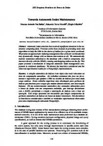
Figure 1.1 represents the overall architecture of the proposed signalling maintenance planning framework for migration to ERTMS. The presented architecture is an answer to the key question: "How to develop a framework to cover scheduling of preventive signalling maintenance tasks for shifting towards ERTMS in the Danish Railway network?"
1.3 Purpose and Contributions
Input
Traffic Optimization Management Module
Dataset
Region Splitting
7
Output A clustered railway maintenance network
Scheduling Framework Preventive Maintenance Planning
Monthly Preventive maintenance schedule
Figure 1.1: Proposed architecture framework for signalling maintenance towards ERTMS Accordingly, the initial input of the system is organised as a dataset. Each dataset mainly consists of a set of geographical points of the crew and tasks locations in the maintenance region. Tasks are either located on the rail tracks, or out of rail tracks or a mixture of off-track and on-track points on the railways network. The proposed framework consists of a planning module which is broken down to two sub-modules of "Region Splitting" and "Scheduling Framework". The first module relates to partitioning techniques used for region splitting as a pre-phase to the scheduling phase. Accordingly, the "Region Splitting" module takes into input a data set and outputs the clustered signalling maintenance tasks. The second module which is the scheduling framework employs the result of clustering as an input and generates the monthly plan for preventive signalling maintenance tasks.
1.3.1.1
Region splitting
The first contribution of the thesis is a partitioning technique used to do region splitting as a pre-phase to the scheduling phase. This idea was developed after the emergence of an industrial need to categorise sub-regions based on the tasks and the crew locations. This is particularly motivated by the fact that the maintenance planning problem at hand takes place in Jutland, the biggest region of Denmark, with a decentralised maintenance structure, where the crew start their duties from different locations rather than starting from a single depot. This is how every partition signifies the different tasks that are allocated to a particular crew in the form of a cluster representative.
8
Introduction
On this basis, two research papers have addressed the clustering problem: 1. Heuristic approach: The clustering problem for a maximum of 5000 tasks can be resolved by employing a perturbative clustering hyper-heuristic framework. 2. Exact approach: To resolve the clustering problem for a maximum of 1000 tasks, a Mixed Integer Programming model has been proposed.
1.3.1.2
Constructive scheduling framework
The second contribution of the thesis is to introduce a scheduling framework for solving the preventive signal maintenance crew scheduling problem. We first model the problem as mixed integer optimisation model. Using this model, there can be a shift from the present system to the ERTMS compliant maintenance planning system when there is a complete adoption of ERTMS. It is described how a preventive signalling maintenance crew scheduling problem can be considered as a Multi Depot Vehicle Routing and Scheduling Problem (MD-VRSP) that has synchronisation constraints. The given problem involves the assumption that the crew members are supposed to resume operating from their homes in the mornings and then go back home once their workday ends. Therefore, the crew homes can be taken as depots, while planning days may be taken as vehicles. There are essentially two distinct kinds of maintenance tasks: tasks that cannot be performed by a single crew member alone which gives rise to synchronisation requirements, and those tasks that can be carried out by only one crew member. It is believed that this research is the first to develop MD-VRSP which has synchronisation limitations particularly in a multi-days’ time frame. Since the PSMCSP generalises the Travelling Salesman Problem (TSP) which is well-known to be NP-hard (Gary and Johnson 1979), it is not expected that the problem can be solved efficiently, i.e. in polynomial time. Hence, a stagewise constructive scheduling framework based on Constraint Programming is adopted to solve the problem for realistic problem instances. In the first stage, a clustering model is solved to allocate tasks to the crew on the basis of their spatial proximity. Clustering leads to a significant decline in the amount of possible permutations of travelling arcs amongst tasks. Next, the proposed framework solves the scheduling problem cluster by cluster, respectively according to a defined order. The framework has been tested on 9 data sets and the results indicate that it is possible to use this two-stage approach to generate an initial feasible solution for realistic problem sizes up to 1000 tasks in a reasonable time.
1.4 Scope and Limitation
1.3.2
9
Scheduling Framework based on Colour-light signalling
The third contribution of this thesis is developing a hybrid Constraint Programming/Mixed Integer Programming approach for maintenance of the existing signalling system in the Danish railway system. The model formulation is a practical mathematical model suggested by a maintenance planner in Banedanmark(Banedanmark 2016), the industrial partner of this PhD research project, and takes various objectives for balancing a crew’s workload, minimising number of working days, crew dimensioning and several managerial constraints into account. The formulation of the preventive signalling maintenance crew scheduling problem for the existing signalling system in Denmark is based on a mixed integer optimisation model. The crew start their tasks from a depot location. Three aspects of the problem add to the complexity of the model. First, the plan includes temporal dependencies between different crew members. There are several crew members that rely on one another as there are certain tasks which may require collaborations between different crew members because of the need for different skills and/or due to safety regulations. Secondly, the traffic requirements can be fulfilled by having a mutual collaboration between the crew to implicitly decrease the possession time of the trains. Accordingly, there is a possible range of crew members to fulfil the tasks per day. Third, the majority of the tasks take much longer than one day and hence, a plan needs to be split over several days. For operational purposes, it is required to produce plans on a monthly basis. In addition, for practical problems, exact solutions are not available. Therefore, a hybrid model is presented in this thesis which employs Constraint Programming for producing initial feasible solutions and considering them as the preliminary warm start solution for CPLEX (via GAMS) for further optimising the solutions.
1.4
Scope and Limitation
In this study, the concern with preventive planning of the maintenance activities is limited to the signalling maintenance tasks. Although, some characteristics of the ERTMS are considered for dealing with possible failures in the region splitting phase of our proposed framework, we must note that the corrective maintenance planning is out of scope for this research.
10
Introduction
In this research, while we consider the maintenance activities for the track equipment, needed for the ERTMS implementation, we do not focus on the maintenance of railway tracks. This particularly means that our study does not deal with the long-term project planning. Rather, our focus is on short term planning (as a tactical problem) and the time horizon of a monthly plan for both of the presented scheduling frameworks Obviously, the operation and maintenance tasks are connected to each other and their connection is inescapable. Two research categories have been identified in the literature, based on the way tactical issues are correlated to the train traffic (Liden 2014). These are: “possession scheduling for coordination with the traffic on the basis of maintenance scheduling”, and “maintenance vehicle routing and team scheduling, in which the concentrated depends on handling resources efficiently”. In this thesis, the focus on vehicle routing and team scheduling is seen as a tactical problem. The emphasis is on the ensuing research spectra, i.e. "managing resources efficiently”.
1.5
Thesis Organisation
This thesis is organised into two parts. The first part gives an overview of the context of the study, including the railway signalling systems, the maintenance planning problems in Denmark, the methods and approaches applied to address the challenges, the current state of the art, and the conclusion of the thesis. These aspects are organised into the following chapters:
• Chapter 2 : Background This chapter briefly introduces an evaluation of railway signalling systems towards the ERTMS for regulating trains and command systems in Europe. Afterwards, it discusses the railway maintenance planning, and the signalling maintenance planing for ERTMS. • Chapter 3 : Signalling Maintenance Planning in Denmark This chapter details the two key maintenance scheduling problems that are addressed in this thesis. It focuses on the challenges and characteristics of the maintenance planning problem applicable for shifting towards ERTMS within the Danish railway system. Furthermore, it addresses the maintenance scheduling problem to deal with the existing signalling system in Denmark.
1.5 Thesis Organisation
11
• Chapter 4 : Methods Involved This chapter mainly introduces two approaches utilised in this thesis, including Hyper-heuristic and Constraint Programming (CP). It elaborates on the core concepts of CP namely, Constraint Propagation, Global Constraints, Constraint Satisfaction Problems and Constraint Optimisation Problems. In addition, it introduces a CP library, called Google-OR tools, which has been used in this thesis. • Chapter 5 : Literature Review This chapter presents the current state of the art and the related literature to this thesis. • Chapter 6 : Conclusion This chapter concludes the thesis with a brief summary of the presented research, the novelties of the work and its contributions, and some suggestions for future work.
The second part of this thesis presents the contributions of this work as a set of academic papers as follows:
• Chapter 7: Clustering of Maintenance Tasks for the Danish Railway System. Published in proceeding of International Conference on Intelligent Systems Design and Applications. (Shahrzad M Pour and Benlic 2016)
• Chapter 8: A Choice Function Hyper-heuristic Framework for the Allocation of Maintenance Tasks in Danish Railways. Published in Journal of Computer & Operations Research. (M. Pour, Drake, and Burke 2017)
• Chapter 9: A Constructive Framework to the Preventive signalling Maintenance Crew Scheduling Problem for the Danish Railway systems. Shahrzad M. Pour, Kourosh Marjani Rasmussen, John H. Drake and Edmund K. Burke. Submitted to Journal of the Operational Research Society.
12
Introduction • Chapter 10: A Hybrid Constraint Programming/Mixed Integer Programming Framework for the Preventive Signalling Maintenance Crew Scheduling Problem. Published in European Journal of Operational Research. (Shahrzad M. Pour et al. 2017)
Additionally, Appendix A provides information about the dataset used for signalling maintenance of the railway system in the biggest region of Denmark, Jutland. It presents information on how the dataset is created and how the software application generates each data file. Data generation is explained through a step by step guide along with snapshots.
Chapter
2 Background
This chapter starts with a brief introduction to railway signalling systems. Afterwards, it explains the evolution of railway signalling systems towards the ERTMS for regulating trains and command systems in Europe. Later, it focuses on the railway maintenance planning, and more specifically the signalling maintenance planning for ERTMS.
2.1
Railway Signalling System
The telegraph was called a “critical companion of railways” in the UK in 1856 (Unknown 1856) following the foremost operational application in 1838 (Unknown 1840), which also played an important role in this regard. The foremost commercial application for the telegraph in the UK railway network was support for the interrelationship between railways and the signalling mechanisms. The signalling system is vital in determining the efficiency of a railway system as it serves as a safety element that aims to ensure safe travelling, operations and security of rail traffic. The signalling system helps in achieving this goal by regulating and supervising the entire railway system using two interconnected layers which process and transfer the information regarding the train and authority movements all across the network. The signalling system does not have an
14
Background
atomic arrangement, but is made up of different sub-components, the principal functionality of which is built upon the interoperability between these (Morant 2014). Sub-components of a signalling system are:
• Traffic management system: the traffic management system manages train traffic, looks after the railway network and create a schedule for the trains. After a route has been determined by the traffic management system, the plan and the required information is given to the interlocking system. • Interlocking system: the network’s safety is determined by the interlocking system. Therefore, when a scheduled route is established by the planners, the interlocking system needs to check it before it can become operational within the network. The system also needs to be aware of whether the train is operating on its track or not, and this is done by the train detection system. • Train detection system: the train detection system such as axle counter or track circuits are designed to determine if the track sections are occupied or unoccupied. Keeping this in mind, when all safety requirements are fulfilled, the train will be permitted to travel on a particular track by the interlocking system. • Psychical signal system: point machines are developed as the physical part on the tracks which ascertain the direction taken by the train by fixing the track switches. Eventually, the train drivers are cautioned by the signals that are depicted distinctively, based on the standard of the signal system utilised. For example, a colour-light signal system depicts the signals on the wayside signals that are set up at specific distances on the train tracks.
To optimise the maintenance of the whole railway system, the railway system managers needs to be aware of the functional relation between the various sub-systems as well as the entire system so as to optimise the maintenance of the entire railway network. Since the railway networks were established, various signalling communication technologies have been designed. Initially, the telegraph was developed, followed by the manual system like hand signals and position lights. There was then a gradual shift towards analogue systems, followed by the digital-electronic based communication systems (Clark 2012).
2.1 Railway Signalling System
15
This has led to the development of various standards for railway communication systems that moved from the telegraphic phase to the present-day communication systems such as colour-light signals as well as the wireless radio (Theeg and Vlasenko 2009). Considering the fact that the signalling system is the component for safety, it is crucial for managers to have accurate information regarding the relationships between the sub-elements and the way the work processes take place within them. This has led to the development of various standards particularly in the signalling system so that there can be standardised interoperability between the different components of the signalling system (Theeg and Vlasenko 2009), (Zimmermann and Hommel 2005). Over the years, the communication technologies and the control signalling systems have undergone considerable improvements. This has led to more reliable railway systems and provided more extensive information to provide advanced high speed railways.
2.1.1
Evolution towards ERTMS
This subsection briefly presents the gradual change that is taking place from a colour-light signalling system to ERTMS. This development is explained according to the challenges of the existing signalling systems and the emergence of new communication technologies in the railway sector.
2.1.1.1
Colour-light
At present a majority of railway communication networks relies on colour-light signals (Theeg and Vlasenko 2009) which were first introduced in 1930 (M 1930). These colour-light signals are a better option compared to the earlier mechanical signals as they can exhibit the same features at night as they do during the day. In addition, their maintenance is not very expensive. These signals use the typical green, yellow and red light standard to signify going ahead, getting ready to observe the following signal as red, and then stopping, respectively. Nonetheless, in different countries in Europe, there are different fundamental features of colour-light signal, and at times, these aspects are contradictory to each other. For example, in Sweden and Denmark, there are contrasting meanings of the single green and double green light. Because of the absence of
16
Background
a coherent signal communication standard, the cross-border interoperability of railways decreases since drivers cannot operate in the two countries if they are unaware of the signal standards of each country.
2.1.1.2
Automatic Train Protection
In the 1980s, Automatic Train Protection (ATP) was adopted in Europe, with the intention of formulating communication technologies for digital systems that were in line with the need to have greater supervision of train drivers. The ATP system carries out supervision of trains, a concept that emerged in 1944 (Horn 1944). It enhances train safety by consistently keeping an eye on the speed of trains and issuing warnings to the driver if they go beyond the speed limit (Hollands 1988). There is an automatic brake installed within the ATP which carries out the braking action when there is no response from the train driver to the warning (Newman 1995).
2.1.1.3
In-cab Signalling
The ATP feature can be implemented when the train drivers have extensive information with respect to the speed limit and the movement authority. This brought about the in-cab signalling feature (Chester 1956) in trains. It is not possible to transfer extensive information just through colour-light signals, rather, a digital communication system is needed between the train driver and the Train Control Centre (TCC) to ensure the operability of ATP or cab signalling feature. Over the years, a tailored ATP system has been developed by each country on the basis of their national needs, and based on the different technical and operational regulations which are essentially not consistent between countries. This serves as a significant hindrance in carrying out the integration of the European signalling railway system to make it a single coherent standard (Winter et al. 2009).
2.1.1.4
Mobile Communications-Railway
The Global System for Mobile Communications-Railway (GSM-R) is the latest digital standard for railway communication which seeks to take the place of the various analogue systems that are present in Europe today. The EIRENE – MORAINE specifications form the basis of the requirements and the standards that are needed to ensure the operability of the GSM-R (Theeg and Vlasenko
2.1 Railway Signalling System
17
2009). EIRENE identifies the “Technical Specification for Interoperability” (TSI) as ", which is the series of requirements which have to be met to ensure their consistency with the rest of the European networks"(SRS 2006). The introduction of GSM-R makes the direct communication between trains and the Traffic Management System possible. This subsequently offers the possibility for establishing new command-control systems which can support and manage train drivers.
2.1.1.5
European Train Control System
The absence of a mutual interoperable ATP system between European countries, apart from the ability of the GSM-R to encourage real-time communication, compelled the European Institute of Railway Research to create a signalling control and train protection system at the end of 1990 (Kane, Shockley, and Hickenlooper 2006). The Union Industry of Signalling (UNISIG) was created in 1998, which had the objective of determining the specification required for executing the latest Train Control System. As a result, the European Train Control System (ETCS) was established to fulfil the requirement of having interoperability between high-speed rail as well as between the traditional rail system (System Requirement Specification 2016). Union Industry of Signalling (UNISIG) has published the System Requirement Specification(SRS) which was needed for ETCS adoption. The latest version dates back to 2012 in SUBSET-026 (SUBSET no date). The standards include the specification for Reliability, Availability, Maintainability and Safety (RAMS) of the all sub-systems of a railway system. European standards included in the SUBSET-026 specifically on safety include:
• EN 50129:2003 "Railway applications – Communication, signalling and processing systems – Safety related electronic systems for signalling" • EN 50128:2011 "Railway applications - Communication, signalling and processing systems -Software for railway control and protection systems"
The approval procedure for individual systems are explained in the EN 20129 as per the technical specifications, considering the railway control and protection system as a whole. Software operability is particularly emphasised so as to fulfil the requirements for safety.
18
Background
In the EN 50128:2011 standard, the specifications for safety-related software that is employed for railway control and protection systems are given. These are related to the organisational structure, organisational associations, deployment and maintenance functions, areas of responsibility for growth and competencies required from staff members. Even though it is critical to have interoperability within the current railway signalling system because of their duty to regulate and monitor the network, the railway networks start to depend more on communication technologies. The main reason for this is that wireless telecommunication technologies have been used in the past few years, which creates the potential of using further advanced railway communication-based services (Sniady 2015). Some examples of such advanced services include: the use of video surveillance (Aguado et al. 2008), cargo tracking (Kurhan 2015), and electronic ticketing mechanisms (Calle-Sanchez et al. 2013). Further examples of such services that may or may not be deployed in the future in railways systems are given in (Sniady 2015). It is evident that a reliable signalling communication system gives rise to a successful and stable railway system. On the other hand, when the signalling system undergoes frequent breakdowns and failures, the performance of the entire railway system can be affected. Hence, a significant role is played by any investment made on the design level, renewal or maintenance features of the signalling system.
2.1.2
ERTMS
A distinct European standard has been put forward by the European Rail Traffic Management System (ERTMS) for regulating train and command mechanisms in Europe. It is backed by the EU with the intention of improving safety and performance of trains, and inter-functionality of rail transport across borders (Bloomfield 2006). There are two key components of the ERTMS; ETCS and GSM-R, the foremost being a condition for in-cab train control, with the latter being a GSM mobile communications condition for railway operations. A safe maximum speed is continuously determined by the ETCS for every train, while there is cab signalling for the driver and on-board systems which take action when the train speed increases beyond the prescribed limit. ETCS consists of various new sub-elements of ETCS, like Driver Machine Interface (DMI) as a component of In-Cab signalling, the Radio Block Centre(RBC), Eurobalises and On-board Unit(OBU).
2.1 Railway Signalling System
19
ETCS can be executed when trackside equipments and train systems are standardised on the basis of various ETCS levels. ETCS basically has three levels, with the third one still being in the conceptual stage (Zimmermann and Hommel 2005): 1. ETCS Level 1: is track side executed and ETCS balises help in transferring data from track to train. 2. ETCS Level 2: a radio based system in which an in-cab screen displays the signalling and movement authorities. 3. ETCS Level 3: a completely radio based system in which the track side equipment is eliminated. GSM-R includes two elements: GSM-R voice and GSM-R data. The existing analogue systems will be substituted by GSM-R voice, which makes certain that there is advanced radio communication between the driver and the corresponding remote control centre, and the staff members through the speakers. This system is closed in nature and is only employed in railway operations to improve the overall security of the system (SRS 2006). GSM-R data is an advancement of GSM-R voice and makes certain that there is ensuing communication over the network. It is a part of the Banedanmark replacement program explained earlier(Banedanmark 2009). Because of the overall restorations of hardware in ERTMS, it becomes imperative to re-examine the entire maintenance scheduling so that it can be modified as per the latest signalling system. This subsequently leads to the need to have new Operations Research tools so that ideal maintenance plans can be created in the new signalling program.
2.1.3
Danish Signalling System
According to Banedanmark, approximately 560 trains are operational in the Danish railway network, which belong to four operators on a track that is almost 3200 km long and has almost 2100 km of lines(Banedanmark 2009). The foundation for the present Danish signalling system is the national Automatic Train Protection (ATP), also known as Automatic Train Control (ATC) that follows the Siemens ZUB100 platform(Banedanmark 2014). ATC was enforced in Denmark between 1986 to 1988, which is over fifty years old (Banedanmark 2009). In another part of the Danish railway network, relay technology was used since the 1950s-60s, while a few even employed technologies from the start of the 20th century (Banedanmark 2009).
20
Background
From the perspective of the sub-system, the current signalling system includes a traffic management system, axle counters in the form of a track detection system, the interlocking, colour light signalling, and electric point machines, which are the physical signal system. Banedanmark’s rule book SR-75 explains the standardisation for employing colour-light signalling in the present railway system (Banedanmark 2009). At present, there are over 20 distinct train control systems being employed in Europe, and there is no harmony between them (Zimmermann and Hommel 2005). On a similar note, the ATC system in Denmark is not consistent with its neighbours, Sweden and Germany (Siemens.dk no date). Hence, when trains are going past the border, they have to be knowledgeable about the two distinct ATC systems. Since the systems are becoming older, over half of the signalling assets’ will expire in the next 15 years (Banedanmark 2009). 50% of the delays that are faced by Banedanmark’s customers annually are due to the existing signalling system; this amounts to almost 39000 delays (Banedanmark 2009). On this basis, the Danish government performed a comparative assessment of a partial renewal of the existing signalling system basis on the life cycle expiry of the previous system, and a complete renewal of the whole signalling system. It was decided to do a complete renewal as this is more beneficial with respect to cost, risk and benefits (Banedanmark 2009). It was decided in January 2009 that the renewal project should be carried out before 2021 (Banedanmark 2009). The concept of complete renewal is adopted by the replacement program, meaning that all the signalling equipment should be renewed. The reason for this was not just the age of the signalling equipment, but also other related issues like costly maintenance activities, decreased safety, and lack of experience and skills for the previous equipment as staff members retired. The complete renewal plan suggests that each of the system’s equipment should be replaced with new ones, regardless of their age. This will ensure that all equipment conforms to contemporary signalling technology, on the basis of standard industrial hardware elements. This provides consistent system interfaces, complete interoperability and extensive reliability. A complete renewal of the signalling systems will also require a large organisational changes in Banedanmark (Banedanmark 2009). These changes mean there will be a need to develop new competences and recruit new staff members with a new set of skills. It is therefore important that Banedanmark carries out change management activities in order to inform, lead and steer the organisation in the right direction.
2.1 Railway Signalling System
21
The European Rail Traffic Management System (ERTMS) was chosen for replacing the entire system from a line-side signalling system to a sophisticated radio-based signalling system because it provided the option of complete rejuvenation.
Figure 2.1 represents the signalling system on the basis of colour-light and the ERTMS within the Danish railway system. After a route in the colourlight signalling system is decided for a particular train, TCC requests the interlocking system to validate the route. The axle counter determines through the interlocking system if a train is moving on the track or not. When no train is moving on the tracks, the interlocking system will permit the train to travel on a particular track. The route taken by the train is identified by the point machine by establishing the track switches. Lastly, the train drivers are informed when signals are transferred through on the wayside signals which are set up at different locations across the train tracks. The current signalling system is also backed by ATP with the help of ATP-balise and ATP-onboard, and infill loops to support line side signalling.
The Figure 2.1 depicts that ERTMS is formulated over the current signalling system, in which the Traffic Management System (TMS), axle counters, interlocking, and point machines are identical to the colour-light signalling system. A novelty of the system is created by ETCS through two key elements of RBC and EuroBalises as track side elements, with OBU being the on-board equipment. Eurobalises function as “beacons”, by giving the precise spot at which the train is, while the on-board equipment regulates the information transmitted by comparing the permitted train speed. The DMI similarly presents the authority movement to the driver. RBC is also consistently given information from train regarding the speed, the precise position and the route of the train. Through the GSM-R, rapid communication between trains and the train control centre (TCC) is permitted as part of the Traffic Management System.
The key advantage of having in-cab signalling rather than colour-light signals is that it becomes possible to dispatch more thorough information to the driver, such as the speed limit or the precise distances to particular locations, and this has a strong effect on the safety of trains. When DMI is particularly used as an interactive screen, the driver can communicate with the Train Control Centre (TCC). In addition, DMI can obtain and depict information at any time, which is not possible with colour-light signals situated at the fixed positions (Sniady 2015).
22
Background
Traffic Control Center
Traffic Control Center
GSM-R Transmitter
RBC
GSM-R Antenna
Interlocking
Interlocking
DMI
ETCS
ATP-onboard
ATP-Balise
Axle counters
Point machines
Eurobalise
ATP signalling
Balise antenna
Axle counters
Point machines
ERTMS level 2
Figure 2.1: Comparing Colour-light signalling and ERTMS level 2
2.2
Railway Maintenance
To define maintenance standards are described by the European Committee for Standardization (CEN), which include the generic terminologies that are utilised for different kinds of maintenance and maintenance management (Standardization (CEN) 2010). According to the related standard, maintenance refers to maintaining components and systems that include software elements, but not the software on its own. In the maintenance field including maintenance of railway systems, the CEN Technical Committees (TC) has especially called for the creation of a wideranging structured generic maintenance vocabulary standard which involves key terms and their descriptions. It is suggested by the terminologies used in this standard (CEN/TC 319) (Cigolini et al. 2006) that maintenance includes not just technical functions, but also other functions like planning and monitoring. On this basis, the focus of this thesis is planning of signalling maintenance activities within the Danish railway network.
2.2.1
Maintenance Activities
Maintenance activities can be categorised in several ways (Liden 2014). When considering those maintenance activities that occur depending on whether failure has or has not been identified, maintenance activities can either be corrective or
2.2 Railway Maintenance
23
preventive (Standardization (CEN) 2010). Accordingly, preventive maintenance refers to the activities that are carried out to ensure degradation and breakdowns do not occur. On the other hand, corrective maintenance involves the activities that are performed once a need for maintenance has been recognised. There are distinct approaches into which these categories can be grouped, and these are given in the following. Corrective maintenance may either take place instantly, or may be delayed. In the first situation, a maintenance task has to take place immediately so as to prevent huge financial losses and consequences, as well as scheduling deferrals. The second situation, an event may have occurred, but its maintenance has already been decided for a particular time. Preventive maintenance can either depend on a condition, or it can be determined beforehand. In the condition-based maintenance, a mix of condition monitoring and/or inspection and/or examination, analysis and the subsequent maintenance activities are involved. In predetermined maintenance, maintenance activities are performed from time to time at specific instances. These can either be calendar-based, or depend on the extent of operating hours that have passed. Keeping in mind the planning perspective, maintenance functions are classified on the basis of the time taken by the activities and how long they should be planned before the activity is carried out (Liden 2014). The time taken for the task ranges from one hour to several days, while the planning tasks range from making plans one month to three years in advance.
2.2.2
Railway Maintenance Planning
Maintenance team routing and scheduling problems can be explained as a prescribed group of maintenance tasks that require being assigned to a group of maintenance teams (Gorman and Kanet 2010). From the practical point of view, there are various hard and soft constraints that occur due to routing and scheduling aspects of the problem and various managerial constraints with respect to the crew’s abilities and the policies of railway maintenance managers, and these make the problems more complicated. In contrast, there are different objectives which usually have a trade-off with one another, and this increases the intricacy of the problem to such an extent that Mixed Integer Programming (MIP) cannot be used alone to resolve the problems that occur on a huge scale. The problems pertaining to railway maintenance planning and to scheduling are essentially divided into strategic, operational and tactical problems (Liden 2014), refer to Figure 2.2. Strategic maintenance issues are usually related to
24
Background
Figure 2.2: Classification of maintenance planning problems
dimensioning, localisation and organisation constitution that is examined over a span of several years. Time-tabling and scheduling plans are part of tactical problems, and these are normally related to a medium-term time frame, i.e. from weeks to a year. Finally, in the operational category, the issues are related to implementation, and have short-term time frames, such as hours to months. The actual individual resources are usually examined, and there is real-time management. Two research categories have been identified in the literature, based on the way tactical issues are synchronised with train traffic (Liden 2014). These are: “possession scheduling for coordination with the traffic on the basis of maintenance scheduling”, and “maintenance vehicle routing and team scheduling, in which the concentrated depends on handling resources efficiently”. In this thesis, vehicle routing and team scheduling is emphasised as a tactical problem, and is shown in bold in Figure 2.2. The emphasis is on the ensuing research spectra, i.e. managing resources efficiently.
2.3
Signalling Maintenance in ERTMS
The implementation of ERTMS have influenced all aspect of the railway system including a significant effect upon the maintenance aspect. Introducing new hardware mainly in the form of a new on-board signalling equipment, new software, and wireless communication technology in ERTMS, necessitates different maintenance tasks and brings a new generation of maintenance aids and helps into the preventive and corrective signalling maintenance activities.
2.3 Signalling Maintenance in ERTMS
25
As ERTMS is still in the initial stages of being operational in this decade, there is very limited research pertinent to the maintenance process in ERTMS (Tapsall 2003), (Redekker 2008), (Patra, Dersin, and Kumar 2010),(El Amraoui and Mesghouni 2014), (Barger, Schon, and Bouali 2009). The effect of ERTMS on maintenance activities of a signalling system has been examined in (Tapsall 2003), in which the following aids are provided: • Cost-effectiveness: There are various railway operators who can implement the ERTMS. Since the number of elements in ERTMS is less than any conventional existing signalling system, this allows operators to create a greater number of products with fewer expenses, and help with the daily activities while having less maintenance costs. • Less on-board and track-side equipment: ERTMS has a single DMI, and this is quite notable compared to the ATP systems, which have six machine interfaces in the Eurostar train cabs, and eight in Thalys trains. Hence, a greater number of free spaces will be given by the signalling on-board equipment for rolling-stock system. In a similar way, fewer track-side equipment are employed by ERTMS as compared to any other kind of ATP, and this ultimate generates lower maintenance expenses. • Compatibility and Independence: There is consistency between ERTMS and the current signalling systems, however, the ERTMS is simultaneously not dependant to any signalling system based on the current and future track-side equipment. This brings about the eventual shift from the present national signalling system to the ERTMS because of the potential national restriction and the economic standards of various countries. • Saving on amount of maintenance tasks: The radio communication across the on-board equipment creates centralisation of on-board maintenance data between the train and the maintenance depot. Thereby, earlier maintenance actions can be taken into account. On the track-equipment, track staff protection is going to be optimised which brings savings in the track maintenance activities. • Effect on preventive maintenance: There are improvements in preventive maintenance within ERTMS because of the fact that all kinds of equipment, ranging from on-board to track equipment, can be supervised. Due to this, the operators get to know about the condition of every equipment, which allows the maintenance or investigation functions to be carried out instantly. In addition, there can be transfer of on-board equipment to the workshop for the purpose of carrying out maintenance, instead of checking
26
Background them at the track site form any maintenance depot, which is the case in colour-light signal system. • Effect on corrective maintenance: The sub-components of a signalling system are dependent on each other, which is why if one component breaks down, the entire system may stop functioning. When the trains and the crossing areas are supervised by the permanent presence of radio (GSM-R), and when there is communication between the Traffic Control Centre and the drivers, then there will be a significant decline in the number of failures and breakdowns encountered at level crossings and in the scale of their impact (known as the knock-on effect (Jespersen-Groth et al. 2009). When failures do take place, they can be instantly detected in the system, and so, the system manager and the crew members can be informed regarding the activities that have to be carried out.
Chapter
3 Signalling Maintenance Planning in Denmark
This chapter addresses two key maintenance scheduling problems that has been addressed in this thesis. The first section focuses on the challenges and characteristic of the maintenance planning problem applicable for shifting towards ERTMS within the Danish railway system. The second section addresses the maintenance scheduling problem related to the existing signalling system in Denmark.
3.1
Problem Addressed in ERTMS
The maintenance problem encountered in ERTMS is explained by describing the maintenance structure of ERTMS in Denmark. Banedanmark is a company run by the Dainish state and falls under the Ministry of Transport (Banedanmark 2016). The company looks after the maintenance and traffic management of the newly installed signalling system. The signalling replacement program being run all over Denmark has been developed as a single program, however, it has been divided into ten projects and includes several contracts(Banedanmark 2009). The maintenance planning taking place in Jutland involves the association of the Western Fjernbane, contracts with the Thales and Balfour Beatty Rail (Thales
28
Signalling Maintenance Planning in Denmark
B.B.R.) consortium and was established in January 2012 (Banedanmark 2014). This contract involved installing signals on almost 1200 km of rail lines (almost 60% of the Fjernbane lines in Denmark) and maintenance planning in the largest region of Denmark, Jutland(Banedanmark 2009).
Suppliers
CTC Monitoring tools
LEU RBC
Second-line crews
Points/ Train Detection/ Balises
GSM-R
On-board equipment EVC
First-line crews Tasks
POSS
Maintenance Organisation
Figure 3.1: ERTMS Maintenance structure
Figure 3.1 is representative of a maintenance organisation for ERTMS in the Danish railway network inspired from (Redekker 2008). This organisation is based on the description and the schematic view provided by the contractors of the ERTMS maintenance regime in Denmark and Netherlands (Redekker 2008). According to their description, it can be seen that the maintenance staff for ERTMS involves a first-line as well as a second-line maintenance team. The first team is composed of engineers and it carries out maintenance activities pertinent to track equipment, such as point machines, axle counters, balises and signals. The second team involves professionals, like electromechanical engineers who manage more complex tasks, such as the electronic interlocking system and on-board equipment. Since these members are experts, they can manage issues that cannot be handled by the first group of engineers alone. The second-line engineers also have to communicate with various suppliers of GSM-R, European Vehicle Computers (EVCs) and Radio Block Centres (RBC-s).
3.1 Problem Addressed in ERTMS
29
The maintenance regime described in (Redekker 2008) shows that the second-line team members supervise all of the ERTMS elements remotely by using the current monitoring tools. It is possible to link the European Vehicle Computer, the on-board ERTMS system to a preventive monitoring system (POSS) that has been created by Strukton (a railway organisation based in the Netherlands that is working in collaboration with Thales B.B.R.). Through the POSS, the maintenance organisation can monitor the trains by following a straightforward process. It is also possible to supervise the ERTMS track equipment (the RBC) in a similar way when the relevant supplier includes this feature in the safety module.
3.1.1
Need for simultaneous presence of crew members
After investigation of the characteristics of the maintenance organisation for shifting towards ERTMS, and the maintenance regime explained in (Redekker 2008), there are essentially two kinds of maintenance activities in ERTMS, as described below.
• In the first kind of maintenance activities, track equipment such as axle counters, point machines, balises and signals are handled. Such kind of activities can mainly be carried out by the current team members. However, there are certain safety regulations in place, due to which a few maintenance activities require two crew members to be present at the same time when carrying out the maintenance. • In the second kind of maintenance activities in ERTMS, the tasks are more complex and involve the electronic interlocking system and on-board equipment. The current crew members are unable to perform such activities, at least alone. Based on the extent of intricacy of the task, they can be carried out by either one or two professionals from the other group, or may require the expertise of both groups.
It is evident from both kind of tasks that several maintenance activities require the simultaneous availability of two crew members, having the same or different skills, at the maintenance area. This provides operation synchronisation to a task (Drexl 2012).
30
3.1.2
Signalling Maintenance Planning in Denmark
Need for clustering the maintenance region
There can be varied degrees of consistency between the sub-systems of a railway system, depending on their geographic layout (Liden 2014). For instance, it is possible that the signalling system is not within the same layout of the rolling stock because of the variations between the elements (Liden 2014). Therefore, the maintenance activity that is taking place in a signalling component may affect the network in a distinct way, in contrast to the one taking place on the rail track.
In addition, in case of a breakdown, failure of a single component in the signalling system may cause other components to also undergo failure, or may even influence the entire network, which is distinct from what happens when there is failure on a track segment.
Similarly when a breakdown happens failure of one component in the signalling system may lead to the failure of other components or even propagation of its impact on the whole network compared to when a failure happens on a track segment. This differentiation makes the partitioning of each sub-system influential, affecting the levels of operability and the maintainability of the railway network (Liden 2014).
Denmark is composed of a long peninsular (Jutland) and several islands. The country has a particular geography which has a significant impact on the growth of the railway sector in the country. Because of these distinct geographical characteristics of Denmark, the current maintenance planning in the largest region of the country has a decentralised maintenance structure, in which the crew commence their duties from distinct locations instead of commencing from one location.
According to the industrial partner of the project, the maintenance plan should help in defining the sub-regions, in which each crew is working. There should be a balanced work burden in every sub-region, they should be demarcated logically, and the geography of the regions should make certain that the crew can travel from one region to another in a very short time span whenever required by corrective maintenance.
3.1 Problem Addressed in ERTMS
31
Figure 3.2: Maintenance Problem in Jutland
3.1.3
Abstract signalling maintenance problem model
Keeping in mind the features of the Danish railway system and the ERTMS when changing from the current signalling system to ERTMS, Figure 3.2 provides an overview of the abstract model of the maintenance problem in ERTMS that this thesis addresses. It has been explained earlier, that some maintenance activities required in the ERTMS cannot be undertaken only by a single crew, as highlighted in Figure 9.3. As an example, consider that the tasks tn and tm have to be performed by two crew. Hence, even though crew c3 and c4 are supposed to perform single tasks in their own paths, the maintenance plan should be such that it allows coordination between the different crew members/engineers for such maintenance activities. This is how crew c3 and c4 should get in touch with each other at the same time and place in their independent everyday route to carry out these kinds of maintenance activities.
32
Signalling Maintenance Planning in Denmark
Various maintenance tasks should be carried out by every member every day as their monthly routine. In addition, less than two hours are normally spent on a task, with no task being divided over a span of two days. This is how the scheduling problem can be taken as various independent everyday routes that are part of the monthly plan, commence from the site of the crew, provide services to a few tasks and end at the crew site when each day ends. A distinct route signifies every daily plan, and a unique colour is used for a daily route for each staff member. Therefore, since the maintenance problem is spread out over a month, the number of independent paths taken by every crew signify the number of working days every month for the pertinent crew. Maintenance Task PM-Point Machine Ax LX Balise Marker B ToB/TVC TCC track maintenance tasks
Task Type Preventive 95%: Preventive 5%: Predictive Preventive Preventive Preventive Preventive Preventive Corrective
No of tasks 1250 3700 400 4500 4000 200 100 400
Frequency Yearly Yearly 1, 2 or 3 Yearly Yearly Yearly Yearly Yearly Yearly
Table 3.1: Type and frequency of the maintenance tasks The signalling maintenance planning is scoped to a predetermined maintenance plan which is applicable for maintaining the signalling components. According to (Liden 2014), signalling maintenance takes less than one hour of possession time and it needs to be planned within two months prior to be undertaken in the maintenance area.
3.2
Problem Addressed in Colour-light Signalling
In the existing signalling system in Denmark, there are four maintenance aspects considering the maintenance regions: Maintenance Machines, Maintenance Nationwide, Maintenance East and Maintenance West (Banedanmark 2009). There is further subdivision of the East and West divisions into Track Maintenance, Current Maintenance and Signalling Maintenance. In this thesis, the main maintenance area assessed falls under the signalling segment of the West region. Various authors have examined the maintenance team scheduling issues (Gorman and Kanet 2010), (Nemani, Suat Bog, and Ahuja 2010), (Bog, Nemani, and Ahuja 2011), (Peng 2011), (Peng and Ouyang 2014), (Borraz-Sanchez and Klabjan 2012). These authors have put forward various methods and techniques for resolving
3.2 Problem Addressed in Colour-light Signalling
33
these problems. A major characteristic of the maintenance planning problem is working in harmony with train traffic. The railway infrastructure maintenance problem was analysed thoroughly (Liden 2015), and it was found that there are three areas of research that allow coordination with train traffic when tactical problems are encountered; (1) possession scheduling for coordinating with traffic; (2) on-based maintenance scheduling, and (3) maintenance vehicle routing and team scheduling, in which the focus is managing resources efficiently. The models put forward in the literature given above achieve traffic coordination by scheduling a greater number of jobs at the same time so as to reduce the possession time of the railway system. In Denmark, the Traffic department of Banedanmark carries out the planning for traffic and possessions. The maintenance division, known as Banedanmark Production, performs planning for maintenance, including desires for possessions. Those people recruited in Banedanmark Production actually perform the maintenance. At times, maintenance teams provided by contractors are recruited, however, the model is only relevant for the maintenance that is performed by the internal staff members. Therefore, optimal maintenance plans should be developed by the Production Planning department, who should present the plan, comprising of the possession time, to the Traffic division. Accordingly, it is under the third spectrum that the signalling maintenance crew scheduling problem utilising colour-light in railway networks in Denmark is classified. Here, the goal is to handle resources efficiently. It is decided by Banedanmark that the plan presented by the production group should permit allocating a greater number of crew members to a single task so as to decrease the overall time frame of the individual task, instead of planning various tasks at the same time. Subsequently, when possession time is included by the tasks, there is a pleasant side effect which is that there is a decrease in the degree of simultaneous possessions occurring, and also in the time duration of every possession. Hence, possession time is taken to be the key resource that is in a deficit and so, it needs to be decreased. In addition, it is better to decrease the working hours, however, decreasing overall possession time is mostly preferred by the operators and travellers. Allocating a greater number of crew members to a single task is a novel way of framing this problem by decreasing possession time implicitly. This is similar to other approaches presented in the literature. On the other hand, when there are a greater number of crew members who are handling a task, there is a reduced feeling of accountability among them, and hence, the quality of the task declines. Consequently, the greatest possible number of staff members are offered by Banedanmark who can be allocated to a task. In addition, there are safety regulations which assert assigning two
34
Signalling Maintenance Planning in Denmark
crew members simultaneously to the same task. Similarly, the least number of crew members required to do a task (one/two crew member(s)) are provided information regarding each activity within the data set. Keeping in mind the scheduling aspect, the crew scheduling maintenance problem faced in the railway networks of Denmark have various restrictions that need to be dealt with. In every maintenance plan, some amount of labour is required (crew members), and this is a major cost of maintenance. With respect to the time frame, there is very little time that is free for maintenance as another scheduling resource. This is because of different factors, like weather conditions, railway traffic functions, and so on. Accordingly, the objective function is composed of three parts. The number of working days required for implementing the plan should be decreased, as many tasks as possible should be fulfilled within the planning time frame, and the repercussions for making a poor plan from the managerial perspective, should be taken into account. After carrying out several meetings with the industrial partner of the PhD research project, the following restrictions on maintenance activities, crew and scheduling time in the existing signalling maintenance planning in the railway network of Denmark were detailed. At present, over 10,000 maintenance tasks should be performed each year. The number and kind of maintenance tasks in the present system are shown in Table 3.1, including the corrective and preventive maintenance of the entire track equipment. These range from the usual inspection and minor repairs to the failures encountered. This data has been employed in this PhD study to provide an approximate number of the maintenance tasks that are involved in signalling maintenance. Compared to the everyday time frame, the routine signalling maintenance activities can take more than a daily time horizon. Hence, several activities should be divided over a span of few days. The maintenance activities are performed by a number of crew members. Groups of one or more crew members are developed to carry out the maintenance work. There is management of the working hours as a full-time employee works almost 6.9 hours a day. For operational reasons a monthly plan have been requested.
Chapter
4 Methods Involved
In this section Hyper-heuristics and Constraint Programming as main research topics of this thesis have been studied.
4.1
Hyper-heuristic
Hyper-heuristic is an optimisation approach defined as "a search method or learning mechanism for selecting or generating heuristics to solve computational search problems" (Burke, Hyde, Kendall, Ochoa, et al. 2010). The idea is automating the design process of a heuristic search space to solve the extensive variety of computational optimisation problems (Burke, Gendreau, et al. 2013). The expression "Hyper" comes from the fact that an algorithm in a higher level of abstraction automates the search process by assimilating a set of heuristic algorithms commonly known as the low-level heuristics (Burke, Kendall, and Eric Soubeiga 2003). This goal is attained with the help of a hyper algorithm which designs the search space not only by the process of selection and applying the low-levels (Peter Cowling, Kendall, and Eric Soubeiga 2000), but also through merging them or even generating new heuristics (Burke, Hyde, Kendall, Ochoa, et al. 2010).
36
Methods Involved
The term hyper-heuristic was initially proposed by (Cowling and Soubeiga 2000) and addressed the term as "heuristics to choose heuristics". However, the concept of applying multiple approaches with a probabilistic weighting goes back to the seventies when solving a job-shop problem (Fisher and Thompson 1963). The motivation behind proposing hyper-heuristic has been to develop a framework that can be applicable on a variety of problems instead of tackling just one particular problem, which is mostly the case using meta-heuristics (Ross and Marfn-Blazquez 2005), (Burke, Petrovic, and Qu 2006), (Burke, Hyde, Kendall, Ochoa, et al. 2010). The generality of hyper-heuristic is a consequence of dealing with the search space of low-level heuristics as a non-domain specific search space rather than operating on the solution space directly. In order to integrate the idea of automating and building the search methodologies within the hyper-heuristic framework, several researchers have addressed the need for systematic approaches to design the heuristics. Machine learning has been the most used mechanism to design and guide the search space (Burke, Gendreau, et al. 2013). Moreover, introduction of hyper-heuristics has brought new ideas for designing innovative neighbourhoods, generating novel heuristics from the low-level heuristics, and hybridisation techniques to make a balance between intensification and diversification of the search space(Qu et al. 2009).
4.1.1
Classification
Several categorisation of hyper-heuristics have been presented in the literature(Eric Soubeiga 2003), (Bai 2005), (Bader-El-Den and Poli 2007), (Burke, Hyde, Kendall, and Woodward 2010), (Chakhlevitch and Peter Cowling 2008). The most recent addition of a category of hyper-heuristic, offered by (Burke, Hyde, Kendall, Ochoa, et al. 2010), categorises the hyper-heuristics into heuristic selection and heuristic generation approaches. According to the authors, this categorisation is built upon some of the prior categorisations and the fact that hyper-heuristic behaves as a meta layer on the optimisation and machine learning mechanism to make an interface that is pertinent on a class of problems instead of a particular problem instance. Based on this concept, the proposed categorisation can be conceptualised according to two aspects: the context of the heuristic search space, and the source of feedback during the learning process (Burke, Hyde, Kendall, Ochoa, et al. 2010). Keeping in mind the prior categorisations, hyper-heuristics can be arranged into either approaches which focus on mechanisms for selecting the heuristics or approaches which aim at generating new heuristics from existing groups of low-levels.
4.2 Constraint Programming
37
The second level in the same aspect is related to the nature of the low-level heuristics depending on whether they deal with partial solutions for constructing the solutions or with completed solutions for improving the solutions. In this sense, hyper-heuristics can be constructive or perturbative. Constructive hyper-heuristics usually have more sophisticated low-levels as they build a solution step by step from an empty solution. Constructive hyperheuristic should select the most appropriate constructive heuristic at each step of the solution construction till the solution is built. In the perturbative hyper-heuristics, the concern is to enhance the complete solutions which have been generated in a separate phase. Usually in this category, low-levels may be non-problem specific heuristics containing easy to implement operators like add or swap moves. Also they can be tailor-made and sophisticated like meta-heuristics. Regardless of the type of low-levels, the hyper-heuristic framework repeatedly select and apply the heuristics on the present solutions until some stopping condition is met. Hyper-heuristics based on both construction and perturbation have been applied to a wide range of domains in the literature (Burke, Kendall, and Eric Soubeiga 2003), (Burke, Gendreau, et al. 2013). Taking the source of feedback into account, a hyper-heuristic is either a learning or non-learning algorithm if it employs the information from a searching process or not, respectively. Accordingly, non-studying hyper-heuristics are the ones that do not consume any reactions (Burke, Hyde, Kendall, Ochoa, et al. 2010).
4.2
Constraint Programming
Constraint programming (Apt 2003) is a declarative programming paradigm that has been widely used to solve a variety of combinatorial problems, e.g. scheduling, routing, and resource allocations. In contrast to imperative paradigms, where users need to specify an algorithm to solve a problem, e.g., compute a function based on given parameters, in Constraint Programming, users declare a problem and a solver is used to find any possible solutions for the given problem. In this paradigm, a problem is modelled through a set of variables and constraints specifying relations between the variables. Each variable depending on its type is associated with a set of values, called a variable’s domain that can be assigned to the variable. Constraints limit the domains of the variables by specifying the lower bounds, upper bounds, and defining relations between the domain values of different variables. A solver, usually called constraint solver, utilises a set of
38
Methods Involved
systematic search algorithms to assign proper values to all the variables defined in the model, provided that all the constraints are satisfied. If such assignments exist, they will be considered as the solutions for the problem. Constraint programming can solve two type of problems. Namely, constraint satisfaction problems and constraint optimisation problems. In the following sections, the core concepts of Constraint Programming is discussed, and how this paradigm can solve these type of problems.
4.2.1
Constraint Propagation
One of the important concepts introduced in Constraint Programming is constraint propagation (Bessiere 2006), which is a very helpful method to decrease the solution search space for the given problem. The idea of constraint propagation is to limit the domains of variables to the values where their assignment will not lead to an infeasible solution. This is realised by a particular component, called propagator, implemented for each constraint provided by the solver. This component monitors the values of variables restricted by the constraint and removes values from their domains which violate the constraint. For example, the constraint solver provides a constraint called greater which specifies a lower bound value of a variable, e.g. Z > 12. The propagator of this constraint removes all the values from the domain of the variable (Z) which are less than the given value (12). Propagating a constraint may trigger the propagation of other constraints sharing the same variables, e.g. propagating Z > 12 leads to propagating Y > Z which removes the undesired values from the domain of Y as well. The propagation chain stops when there are no more values that can be removed from the domain of the variables. If propagating a constraint, at any points, prunes a domain of a variable to an empty set it will fail the current search.
4.2.2
Global Constraints
Global constraints (Beldiceanu and Contejean 1994) are also one of the core concepts of Constraint Programming. The term “Global” refers to two different aspects. The first is the reusability and commonality of these constraints. In this aspect, these constraints are well-known, and they are formally defined. Therefore, reusing these constraints can improve the readability of the model and the productivity of the modellers. At the moment of this writing, there are more than 354 global constraints referenced by the Global Constraint Catalogue (Beldiceanu, Carlsson, and Rampon 2005). For instance, AllDifferent is one of the well-known
4.2 Constraint Programming
39
global constraints, which ensures that the given variables have different values in a feasible solution, e.g., AllDifferent (v0 , v1 , v2 ) indicates that v0 , v1 , and v2 must have unique values. The other aspect is that these constraints specify relations between a set of variables, and they are combinations of other constraints. For example, AllDifferent can be defined for none-fixed number of variables, e.g., v0 , v1 , v2 , ... , vn , and it can be decomposed as follows: v0 6= v1 , v0 6= v2 , ..., v0 = 6 vn v1 6= v2 , v1 6= v3 , ..., v1 = 6 vn ... vn−1 6= vn
(4.1)
Using global constraints to specify a constraint on a set of co-related variables can improve the search performance. Global constraints implement a particular propagator that utilises filtering mechanisms in order to prune the domains of the related variables. For example, the propagator of AllDifferent constraint monitors the assignments of the given variables. Once a value is assigned to any variable under cover of this constraint, it removes the value from the domain of the other variables.
4.2.3
Search Algorithms
A constraint solver utilises a systematic search algorithm to find feasible solutions for a problem. This algorithm systematically explores all the possibilities of assigning different values to the variables. It iterates through the variables and tries to assign a proper value from the domain of the variable to each variable such that none of the given constraints are violated. If it finds it impossible to assign a value to a variable from the variable’s domain, it backtracks and reconsiders the last assignment. This might eventually generate a complete assignment where all the variables are assigned, and all the constraints are satisfied. Two strategies should be specified for the search algorithm. The first is the order of selecting the variables for assignment. Depending on the problem and the variables, it should be specified how the solver should choose the next variable for assignment, e.g. randomised order, max number of values, min number of values, etc. The other strategy is the order of selecting the values from the domain of a variable for assignment, e.g., randomised order, ascending order, descending order, etc. It should be noted that the search space for the problem is defined by the number of the variables and the size of their domains. Furthermore, constraints can also have an effect on search space, since they can reduce the domain size of the variables.
40
4.2.4
Methods Involved
Constraint Satisfaction Problems
Constraint satisfaction problems (Meseguer 1989) mostly deal with finding feasible solutions, e.g., eight queens puzzle, map colouring problem, crosswords, sudoku, and many other logic puzzles. These problems are specified as a set of discrete variables (e.g. boolean, integer), a set of the respective domains of values (true, false, 1, 2, ..), and a set of constraints (e.g., X < 6, 2 ∗ X + Y = 20). The goal is to assign values to all of these variables such that all of the constraints are satisfied. To achieve this, constraint solvers employ constraint propagation and a systematic search that removes values from variable domains and assigns values to them. If such assignments exist, they will be considered as solutions to the problem. Sometimes, after the search process, some of the variables may have multiple values in their domain, in this case, the solutions are a subset of the Cartesian product of the variable domains (e.g. X = {0, 1, 2, 3, 4, 5}, Y = {20, 18, 16, 14, 12, 10}).
4.2.5
Constraint Optimisation Problems
Besides feasibility, constraint optimisation problems also deal with finding the optimal solutions for the problem among the feasible solutions. Examples of these problems are the golomb ruler problem, the job-shop problem, the travelling salesman problems, and the vehicle routing problems. Similarly, these problems are modelled as a set of discrete variables and a set of constraints; additionally, they specify an objective function (f ) which should be either minimised or maximised. The goal of these problems is to find a solution that satisfies all the given constraints such that the value of the objective function is also optimised. Therefore, the constraint solver may return none or only one solution. Constraint solvers solve these problems by converting them to constraint satisfaction problems. To this end, the solver searches through a set of iterations for solutions that satisfy all of the given constraints, and an additional constraint regarding the objective function. This constraint depends on the type of the optimisation, minimisation or maximisation and is defined as f > v or f < v such that f is the objective function and v is the best value obtained for this function so far. This value is initialised to the upper bound or lower bound of the function in the first step, and later in each iteration it will be set to the value of the objective function for the current solution. The solver keeps iterating these steps until no more solutions can be found. In the end, it will return the last solution obtained (if any).
4.2 Constraint Programming
4.2.6
41
Google OR Tools
Google introduced an open source library for finite-domain Constraint Programming, in September 2010 under the MIT license, called OR-Tools (Omme, Perron, and Furnon 2016). The core of this library is written in C++, and it is also available in Java, C#, and Python. Despite the constraint solver, it allows for using various solvers including linear programming and mixed integer programming. On top of the constraint solver, it provides a set of libraries, e.g. graphs algorithms, vehicle routing, and knapsack libraries, to model and solve various constraint satisfaction and constraint optimisation problems as mentioned before. This library supports the common variable types, and it also offers a set of special types that are proposed for scheduling problems such as IntervalVars to model tasks and SequenceVars to model the orders of the tasks in the scheduling problem. This library implements the standard relational constraints and also most of the well-known global constraints. Additionally, it provides means to specify and implement custom constraints. It is quite flexible and provides mechanisms, e.g., DecisionBuilders, DecisionVisitors and Callbacks to define custom search algorithms. It comes with several predefined search strategies that are useful for various scenarios, and even they can be combined to search a sub-tree of the main search tree differently from the rest of the search. This library utilises a two step approach; first, it select a variable, then it assigns a value to the variable. Therefore, it provides a set of predefined strategies to choose a variable (e.g. Choose First Unbound, Choose Min Size Lowest, etc.), and a next value for the variable (e.g. Assign Min Value, Assign Max Value, Assign Random Value, etc.) More importantly, OR Tools supports local search and it has implemented three well-known meta-heuristics including Tabu Search, Simulated Annealing, and Guided Local Search. Moreover, it provides means for defining a custom local search such as LocalSearch, LocalSearchOperator, and LocalSearchFilter. The before mentioned meta-heuristics are implemented on the basis of these mechanisms, and it should be noted that they will be used when the constraint solver have reached a local optimum. Furthermore, OR Tools offers a particular library dedicated to Routing Problems. This library is proposed to deal with different categories of routing problems including Node Routing Problems, Vehicle Routing Problems, and Arc Routing Problems. It can be used to model and solve various routing problems ranging from the Travelling Salesman Problem (TSP) to even more complex ones such as the Capacitated Vehicle Routing Problem (CVRP) with Time Windows. The library uses a single model to solve these problems, but it provides a set of means
42
Methods Involved
for customising and tailoring the model to a particular problem (e.g. multivehicles problems with specific constraints such as capacities, time windows, etc.). For example, it allows considering some accumulated quantities along the routes by introducing the concepts of Dimensions, which are a set of variables associated with each node of the graph to specify certain quantities e.g., weight, distance, time. Since the library is developed on top of the Constraint Programming library, within a class called RoutingModel, it is possible to restrict the inner model with a set of problem specific constraints as well.
Chapter
5 Literature Review
This chapter presents the current state of the art and the related work of this thesis. It covers Maintenance Vehicle Routing and Scheduling Problems, Vehicle Routing Problem and its two variations of VRP with Time Window and Multiple Depot and VRP with exact synchronisation. Furthermore, the chapter provides literature on Constraint Programming on certain specific problems and domains.
5.1
Maintenance Vehicle Routing and Scheduling Problem
Maintenance team routing and scheduling issues are considered to be a set of maintenance tasks that are to be assigned to a group of maintenance staff members having particular skills, keeping in view certain objectives. These objectives can be a mix of routing objectives, such as distance travelled, as well as scheduling objectives, like the working hours of the crew members, in addition to different managerial objectives. In addition, decreasing the disruption time of travelling, known as possession time, is constantly emphasised, either implicitly through management of resources, or clearly in the objective function.
44
Literature Review
Despite the fact that the maintenance Vehicle Routing and Scheduling Problem is an unavoidable task in a railway system, it was not till 2009 that this topic was examined in this context. In signalling maintenance, in particular, there have been no studies that examine the planning stage of the signalling system. Hence, all the reviewed research below have been proposed for track maintenance planning. The foremost study carried out in this domain was by Li et al. in (G. Li, Balakrishnan, and Roth 2009), where track maintenance was stressed upon by suggesting an annual plan that was distributed into days or weeks. A time-space network (TSN) framework was used by the authors to deal with the Production Team scheduling problem (PTSP). This model consists of three kinds of costs and three kinds of simultaneous and precedence side constraints. For solving the problem using MIP solver, the network and side constraints were integrated by the authors, and subsequently, there was a considerable decrease in the extent of variables and constraints. An identical version of PTSP was subsequently examined in (Gorman and Kanet 2010). Here, the focus was on long-term planning of renewal projects. The research used two problem constructions of a TSN mixed integer program, in addition to job scheduling. Integer programming was also used to resolve the problem on the basis of the initial formulations, Constraint Programming, and genetic algorithms used in the job scheduling framework. A down-scaled problem instance was used to compare the suggested methods, were improved outcomes were obtained with the TSN mixed integer program with a MIP algorithm that address large-scale real-life problems, taking an acceptable amount of computation time. In (Nemani, Suat Bog, and Ahuja 2010), the curfew planning problem (CPP) was studied for railway track maintenance. In the CPP, planning pertaining to a set of disruptions was carried out, using a specific number of crew members having a specified skill-set. Every disruption is divided between the various crew members, with the aim of decreasing the overall disturbances in train routes. Three distinct frameworks were examined by the authors (time-space network, set partitioning with alternate work responsibilities for every project and column generation with team routes in the form of columns), in addition to a decomposition approach that depended on the set partitioning model. CPLEX was used to resolve the four solution models, where outstanding results were obtained in the final model in contrast to the rest of the models. Four algorithms were presented by the authors in (Bog, Nemani, and Ahuja 2011), which are used to resolve the identical CPP problem in an iterative manner, involving a back-track technique. Analysis of the mutual exclusion, time windows and precedence constraints were carried out, being a part of the
5.1 Maintenance Vehicle Routing and Scheduling Problem
45
problem. The objective was to achieve the lowest network disruption to generate a yearly timetable. The outcomes achieved were promising, having a successful computational time on real data instances of the North American railroad. In (Peng 2011), a PhD dissertation was given, which concentrated on three optimisation scheduling issues in track maintenance. To resolve the Track Inspection Scheduling Problem (TISP), Job-To-Project Clustering Problem (JTPCP) and Production Team Scheduling Problem (PTSP), several mathematical approaches and solution algorithms were put forward. Various side constraints are a part of TISP, which is a routing and scheduling problem that examines the railroad network with the help of a group of expert crew members. The TISP was developed by the researcher as a VRP model and it was suggested that a two-step methodology should be used to develop and optimise the solution on a broader scale heuristically. The problem is resolved using a constructive heuristic and iterative local search approach. The objective of PTSP is to have long-term planning for capital track maintenance. The PTSP was resolve by considering the problem as a time-space network (TSN) model which was managing various side constraints. In (Peng and Ouyang 2012), a multiple neighbourhood search algorithm was developed to deal with data instances on a wider scale. There are two stages of the optimisation model. The preliminary solutions are obtained using a straightforward scheduling model, and subsequently using two local search algorithms to make the solution optimal. This study follows through the simple heuristic that was presented by the same researcher in (Peng, Kang, et al. 2011). A huge improvement was observed as compared to the usual methods utilised. There is a close link of JTPCP with TISP as well as PTSP, and its objective is to group extensive amounts of capital track maintenance activities into projects (the projects can subsequently be planned as PTSP). A multi-stage approach was then put forward, which included three steps, i.e. the tasks were clustered, the problem was formulated as VRP, and the problem was resolved using the local search method and a task-reshuffling technique amongst the team members. This solution was used in an actual case and a suitable outcome was obtained in an appropriate calculation time. A mixed-integer mathematical programming model that relies on VRP formulation, with additional side constraints, was put forward in (Peng and Ouyang 2014). The problem was solved using three distinct heuristic methods; a local search heuristic, a greedy heuristic and a feasibility heuristic.
46
Literature Review
In (Borraz-Sanchez and Klabjan 2012), one more hierarchical solution approach has been put forward. To reduce the different expenses that are incurred because of having to perform the maintenance activities in a prescribed time frame, the Railway Maintenance Scheduling Problem (RMSP) has been considered as a job-time network model. There is heuristic creation of appropriate solutions, which meets numerous industrial needs using a multi-step module: a network node constructor, a Dynamic Programming-based shortest path procedure, and the insertion, swap and raise flexibility techniques. Using this framework, the different problems encountered over the year were resolved, including over 1000 tasks and involving over thirty staff members. A rail track inspection scheduling problem (RTISP) was examined in a research study presented by (Lannez et al. 2015) following which, a matheuristic method that relied on Benders and Dantzig-Wolfe decompositions methods was presented to resolve the problem for a practical size. The performance of the algorithm was assessed and compared with a dynamic programming-based heuristic. In (Camci 2015), a maintenance planning problem was explained with respect to the assets that are spread out in a geographic region. The failure probability of every asset is predictable, and various assets should be managed by every crew member. The time taken for tasks and degradation prognostics were taken into account in this problem. To suggest a time frame for a geographically distributed asset, a genetic algorithm was used by taking into account the task duration and travelling expense. A large number of tasks could be planned by the algorithm. A maintenance interventions for track geometry correction (TGC) was initially discussed by Santos in (Santos, Teixeira, and Antunes 2015). The objective of this was to decrease travelling costs and the number of working days by as much as possible. It was suggested to use a Decision Rules Model (DRM) on the basis of maintenance regulation in a practical scenario. A heuristic approach was used which effectively decreased the huge cost of the maintenance schedule across the whole annual period. Beside the problem of Vehicle Routing and Team Scheduling in the railway field, a detailed analysis of the activities related to railway maintenance has been explained from the angle of planning and organising in the study in (Liden 2014). The writer has discussed the categories of tasks performed relating to maintenance and provided a catalogue of identified planning and scheduling problems in the railway domain. In addition, the author has conducted a detailed study of already done work in this particular area by researchers so that current approaches could be categorised. Later, the same author has presented a survey of planning problems (Liden 2015) related to railway infrastructure maintenance,
5.2 Vehicle Routing Problem with Time Window
47
emphasising the way various methods tackled the coordination with train traffic operation. A mathematical model and methods of optimisation have been adopted so as to solve the planning problems by examining more than 60 studies.
5.2
Vehicle Routing Problem with Time Window
The vehicle routing problem (VRP) is a combinatorial optimisation problem which seeks to optimise a set of routes for a set of vehicles to travel in order to deliver items to a given set of customers. This section details reviews on only two variations of Vehicle Routing Problems with Time Windows (VRPTW); 1) Multiple Depot and 2) synchronisation constraints. VRPTW is basically a NP-hard problem, which is why these two problem variations are the same (Lenstra and Kan 1981).
5.2.1
VRPTW with Multiple Depot
In this variant of the problem, known as MDVRPTW, the vehicles start and end their routes at varied depots. Various heuristics have frequently been constructed to solve this type of VRP first described by (Cordeau, Laporte, and Mercier 2001). The author suggested an Adapted Unified Tabu Search Algorithm (UTSA) to solve the periodic VRPTW and MDVRPTW. During the research process, infeasibility on the obtained solutions is permitted in the proposed UTSA. By using basic neighbourhood, UTSA becomes a simple and robust solution approach. It was shown that how simple the modified version of UTSA could be employed for each of the three problems for large-scale occurrences, without taking a lot of computational time. The foremost usage of Variable Neighbourhood Search (VNS) (Hansen and Mladenovic 1999) to resolve the MDVRPTW was presented in (Polacek et al. 2004), in which a straightforward local search was carried out in the algorithm. The findings were contrasted with Tabu Search (TS) on practical data instances, which suggested that VNS may be an appropriate solution as improved solutions were attained with respect to quality, and the computational time was also satisfactory.
48
Literature Review
A hybridisation of various VNS and TS was subsequently put forward in (Timmermann and Schumann 2008) to deal with the MDVRPTW. The suggested model was examined using different static and dynamic senarios. Dynamic senarios considered various changes in input, like modifications to customer requests, the number of customers or visiting different customers. It was found that when used for the same MDVRPTW, improved findings were obtained through this hybrid method compared to the UTSA presented in (Cordeau, Laporte, and Mercier 2001).
In (Hong and Xu 2008), a more complicated form of MDVRPTW was modelled and worked upon, taking into account the fuzzy travel time and time-dependency. It was suggested to use a hybrid model which considered genetic and ant colony algorithms, providing appropriate solutions in an appropriate calculation time.
The state of the art approach on MDVRPTW is a hybridisation of Genetic Search with Advanced Diversity Control presented by (Vidal et al. 2013) where their results outperformed all of the current state-of-the art approaches in the literature with respect to the solution quality and computational time. The proposed hybrid method has been successfully applied to a wide range of MDVRP variations including MDVRPTW.
Even though various studies have been carried out on MDVRP, the majority of the studies have not included time-window constraints in the problem (Cordeau, Gendreau, and Laporte 1997), (Yu, Yang, and Xie 2011), (Ombuki-Berman and Hanshar 2009), (Surekha and Sumathi 2011). Adaptive Large Neighbourhood Search (ALNS) (Pisinger and Ropke 2007) has been one of the most promising approaches and is well-known due to its simplicity and its wide range of applicability on several variations of VRP. ALNS uses a ruin-and-recreate technique, where neighbours are selected with the help of an adaptive operator.
Considering the problem formation confronted in the MDVRP/MDVRPTW, containing multiple depots, brings the idea about categorising the customers into the number of depots according to their distance (Surekha and Sumathi 2011). This can ease the decision about the customer assignment to the depots, before the planning phase. Consequently, a research topic has been designated to this category known as cluster-first, route-second approaches that will be explained in the next subsection.
5.2 Vehicle Routing Problem with Time Window 5.2.1.1
49
Clustering-based approaches
In real-life having multiple depots can make it hard to select which customers are served by which depot. A way to simplify this is to group or cluster customers based on the distance between them and the depots. Therefore, the MDVRPTW can be viewed as a cluster and routing problem; e.g. first the clustering is done and then the route is determined (Giosa, I. Tansini, and I. Viera 2002), (L. Tansini and O. Viera 2006). However, the best results has been found by addressing both clustering and routing at the same time (Ioannou, Kritikos, and Prastacos 2001),(Salhi and Nagy 1999). Though in large instances (meaning more than 1000 customers), the simultaneous approach fails to work in an efficient computational time. In such cases the problem has to be broken down into multiple sub-problems with respect to the number of depots which can then be solved individually. Several researchers has made use of multi stages approaches embedded with clustering techniques as solution approaches (Yucenur and Demirel 2011), (He et al. 2014), (Surekha and Sumathi 2011), (Yalian 2016), and (Dondo and Cerda 2007). Focusing on the clustering part under this category of solution approaches for solving MDVRP/MDVRPTW, a clustering phase is most often done using assignment algorithms (L. Tansini, Urquhart, and O. Viera 2001). There are four key classes of assignment algorithms used to address MDVR/MDVRPTW problems: 1. Assignment through urgencies: In this approach a precedence relationship is created between customers to ascertain the order in which customers are assigned to depots. Heuristic examples of this approach include: Parallel assignment (Schulze and Fahle 1999), the Simplified assignment (Giosa, I. Tansini, and I. Viera 2002) and the Sweep assignment (L. Tansini, Urquhart, and O. Viera 2001). 2. Cyclic assignment: In this approach a customer is assigned to a depot one at a time in a cyclic way (Giosa, I. Tansini, and I. Viera 2002). 3. Assignment algorithms by differences: In this approach customers are assigned to clusters based on their differences. Examples are based on Coefficient Propagation and Three Criteria Clusterisation (Russell and Igo 1979) algorithms. 4. Transport Problem(TP): In this approach a customer is assigned to depots using TP so that the assignment is done using an exact approach. This means that it is considered how many items needs to be moved from depots to the customers in a way so a customer is serviced by one depot.
50
Literature Review
After a comparative study on several assignment algorithms including TP, it has shown that the total cost of scheduling is strongly dependent on the assignment algorithms (L. Tansini, Urquhart, and O. Viera 2001). Interestingly, obtaining a good final schedule has been shown to not only depend on the algorithms but also on the geographic features of the problem. The authors demonstrated that TP was a better choice instead of heuristic techniques as it is an exact approach and the time consumed to produce the results is computationally short. TP as an assignment approach has been shown to be the best choice because it is an exact method with a relatively short computation time. However, owing to the restriction concerning the size of the data solvable by TP, heuristics are still a candidate solution approach to tackle large scale data instances.
5.2.2
VRP with Exact Operation Synchronisation Constraints
VRP with multiple synchronisation constraints (VRPMs), is a developing variation of VRP, and is now evolving into an appealing reserach area (Drexl 2012). In (Drexl 2012), the author claims that most of the research available with respect to this topic has been developed after 2011. Contrary to VRPs, in VRPMs the vehicles depend upon each other, which illustrate that a change in the route of one vehicle may influence the route of other vehicles too (Drexl 2012). This is referred to as the interdependence problem. Dealing with interdependence problems necessities taking the synchronisation constraints into account. In (Drexl 2012) a classification is presented of different kinds of synchronisation requirements on task, load, operation, resource and movement. In this research study the main target are the techniques which are appropriate and meet the condition of immediate attendance of vehicles at a particular location to perform operation synchronisation or more specifically, maintaining the same arrival time which is known as the exact operation synchronisation. Both exact and heuristic approaches have been proposed to handle the problems with exact operation synchronisation. It has been emphasised that depending heavily on the time required to perform a feasibility check of the routes and re-evaluating the objective function makes the problem even more challenging in heuristic approaches (Drexl 2012).
5.2 Vehicle Routing Problem with Time Window
51
As stated by Drexl (Drexl 2012), in MIP-based approaches there are two ways of modelling this type of synchronisation in the model which are either using an independant time variable or branching on time windows. With respect to implementation of the synchronisation constraints in the proposed scheduling framework for using ERTMS, this research study is motivated by the work of Bredström and Rönnqvist in 2008 (Bredstrom and Ronnqvist 2008) who presented a MIP-based heuristic in a combined vehicle routing and crew scheduling problem. They propose a straight-forward mathematical model for VRSP-TW which is a generalisation of the vehicle routing and scheduling problem (VRSP) with temporal precedence and synchronisation constraints. They have shown that including synchronisation constraints explicitly in the model has a positive impact on the planning. Accordingly, this review is limited to the approaches which uses an independent time variable which is also the case in the approach presented by (Bredstrom and Ronnqvist 2008).
5.2.2.1
Vehicle-independent time variable
The three approaches presented below are MIP-based and they employ the same techniques for representing the aspect of exact operation in their MIP model. These techniques are to employ "one vehicle-independent time variable for the beginning of execution of a task or operation requiring more than one vehicle at a vertex i"(Drexl 2012). Amongst heuristic approaches, Li (Y. Li, Lim, and Rodrigues 2005) presented a meta-heuristic for solving a Manpower Allocation Problem with Time Windows, Job-Teaming Constraints (MAPTWTC) which is a crew scheduling problem closely related to the Vehicle Routing Problem with Time Windows (VRPTW). A job is marked as fulfilled if the synchronisation constraints regarding the need for simultaneous presence of the composite team is met within the job’s time window. The results indicated that construction heuristics used with simulated annealing are a good approach to solve this NP-hard problem. Dohn (Dohn, Kolind, and Clausen 2009) investigated the same problem with the requirement of cooperation between technicians, and all technicians cooperating must initiate the execution of the task simultaneously. The authors presented an Integer Programming model for the problem, which is decomposed using the Dantzig-Wolfe decomposition. A column generation has been the candidate
52
Literature Review
solution approach in a Branch-and-Price framework. Simultaneous execution of tasks is enforced by the branching scheme. The results showed optimality achieved in 11 out of the 12 used data instances. Cortes (Cortes, Matamala, and Contardo 2010) came up with a generalised formulation of a pickup and delivery problem. The model provides the flexibility of exchanging passengers between the vehicles which brings synchronisation constraints into the problem. The paper details a solution method based on Benders Decomposition where the efficiency of the proposed approach is compared with a straight branch and bound strategy.
5.3
Constraint Programming
Operations Research, Constraint Programming can be applied to a multitude of different problems within Operations Research. The problem and domain within Constraint Programming relevant for this research study is as follows: • VRPs with Synchronisation constraints • Scheduling problems • The railway system The following sections provide insight into specific instances of these problems.
5.3.1
VRPs with Synchronisation constraints
In the context of VRP with exact operation synchronisation, Rousseau (Rousseau, Gendreau, and Pesant 2003) put forth a CP approach to solve the synchronised vehicle dispatching problem (SVDP). The synchronisation constraint arises due to a need for distinct team members to assist the disabled passengers at the same time. The researchers note that it is cumbersome to solve the problem by utilising classic local search approaches as the problem will have to be resolved every time a new passenger is inserted into the problem. The authors propose using Constraint Programming in order to formulate the synchronisation constraints which makes the temporal constraints easy to express. Furthermore, as the propagation of synchronisation constraints happens only when it is called, a solution will be generated in an efficient computational time. The researchers suggest utilising a specific kind of insertion strategy for passengers asking to be served, together with an application of local search methods in periods amongst requests.
5.3 Constraint Programming
53
In (Laurent and Hao 2007), the authors address a simultaneous driver–vehicle scheduling problem in a limousine rental company to create a daily plan. A two phase approach is utilised in solving the problem: the first phase involves obtaining the initial solutions by employing Constraint Programming, while the second phase involves the application of a Simulated Annealing algorithm in order to improve the initial solutions. The implementation of the software in real world situations has yielded high quality schedules, which are able to satisfy all the relevant constraints and cover a majority of the trip demands. The schedules also facilitate a decrease in the operational costs, the number of resources needed, the number of upgrades needed and the total idle time. Moreover, these schedules are also capable of handling cancellations and modifications in the trip demands and service delays caused by traffic congestion. The proposed framework was applied in real world situations and yielded high quality schedules, which are able to satisfy all the relevant constraints while decreasing the final operational costs. El Hachemi (El Hachemi, Gendreau, and Rousseau 2011) propose solving an instance of the log-truck scheduling problem using a methodology based on Constraint Programming and integer programming. The problem is an alternate version of a “pick-up and delivery” routing problem. The schedule must ensure that there is synchronisation amongst the log loader and the trucks, so that trucks and the log loaders suffer as little idle time as possible. To solve the problem, initially the distance travelled on deadhead trips is optimised utilising an integer programming approach. Thereafter, Constraint Programming is applied to solve the problem pertaining to the synchronisation of the trucks and the log loaders and the optimisation of the non-value adding idle time costs. The two approaches are then connected by way of global constraints, which are created by solving the integer programming problem and are then applying it to the Constraint Programming model.
5.3.2
Scheduling problems
Van Hentenryck (Van Hentenryck 1989) was among the first who used the Constraint Programming approach for dealing with the domain of scheduling. The subject then received considerable attention from different researchers. Authors in (Kanet, Ahire, and Gorman 2004) did a preliminary review of the topic as well as its usability for addressing the problems of scheduling. The research puts forward the definition of Constraint Programming as “a methodology for preparing and answering a constraint meeting for the discrete type of variables or constrained maximisation issues. It methodically applies logical pattern for controlling and curtailing the space for research as well as enables the deployment of a range of constraints”.
54
Literature Review
Moreover, the authors (Kanet, Ahire, and Gorman 2004) present a general algorithm which can be utilised to solve Constraint Satisfaction Problems through constraint propagation and domain reduction using filtering algorithms for each constraint. The system can be useful for dealing and resolving a range of problems related to scheduling; job shop scheduling, single-machine sequencing, parallel machine scheduling, vehicle routing, and timetabling. These problems are often subject to special constraints such as strict inequality, logical constraints, and global constraints, that are easily modelled using Constraint Programming in comparison to integer programming. The authors (Kanet, Ahire, and Gorman 2004) also points out the differentiation between Constraint Programming and integer programming in respect to their approach for solving NP-hard combinatorial optimisation problems. Constraint programming focuses on constraints instead of the objective function while integer programming models do the opposite. The same research (Kanet, Ahire, and Gorman 2004) has proved that specific attributes of Constraint Programming, for instance using few variables and numerous logical constraints, increases its usefulness for developing models and providing solutions for solving scheduling problems. The research (Kanet, Ahire, and Gorman 2004) concludes that there is much potential for further exploring the domain of Constraint Programming tools and that Operations Research professionals within this field can expand the usage of this approach in scheduling problems. The concept of Constraint Satisfaction Problems (CSP) is introduced by (Brailsford, Potts, and Smith 1999) to practitioners in the field of Operations Research. Accordingly, CSPs comprise of a set of variables, a finite set of values that can be assigned to each variable, and a set of constraints containing these variables. The values that can be simultaneously assigned to these variables must fulfil all of the constraints. Accordingly, (Brailsford, Potts, and Smith 1999) points out various categories of NP-hard or NP-complete combinatorial optimisation problems pertaining to facility location, scheduling, car sequencing, cutting stock, vehicle routing, timetabling and rostering which can be solved using a constraint satisfaction approach. The authors (Brailsford, Potts, and Smith 1999) also highlight that CSPs can be solved either by using traditional Operations Research techniques such as integer programming, local search methods and neural networks or by using Constraint Programming techniques, which involve conducting tree searches coupled with backtracking and consistency checking. The Constraint Programming algorithms can be computationally implemented on various software platforms.
5.3 Constraint Programming
55
Conventional logic programming languages (PROLOG), specialised logic programming languages (CHIP) or general purpose programming languages using specialised tools (ILOG SOLVER in C++) are some of options that can be used. Th paper (Brailsford, Potts, and Smith 1999) also sheds light on the various aspects of modelling and solving CSPs using Constraint Programming. The research study makes a comparison of the different dimensions of Constraint Programming techniques and traditional Operations Research techniques based on certain parameters and identify instances in which the usage of one technique would be preferable over the other. There are different dimensions where different languages vary; however, the authors (Brailsford, Potts, and Smith 1999) consider the most important ones to be implementation ease, flexibility to handle a variety of constraints, computation time and quality of the solution. According to the research, the development of Constraint Programming is limited in comparison to traditional Operations Research techniques. However, it is believed that it is imperative for researchers in the field of Operations Research to realise the potential of Constraint Programming algorithms, and consequently, develop better-performing hybrid algorithms which seek to combine characteristics from algorithms pertaining to both of these fields.
5.3.3
The railway system
Gorman and Kanet (Gorman and Kanet 2010) put forward various techniques which can be used to automate the annual scheduling of rail maintenance production crews. The authors propose formulating the problem in two ways: a time-space network formulation and a job scheduling formulation. The timespace network formulation of the problem could be solved using the mixed integer programming approach, while Constraint Programming algorithms and/or genetic algorithms can be used for solving the job scheduling formulation. This research paper has been reviewed in Section 3.2 where it was detailed that the mixed integer program network formulation yielded the best results in terms of computation time and solution quality. Authors in (Cheung et al. 1999) contribute to the development of the Engineering Work Track Possession Assignment System (EWTPAS) which utilises constraintsatisfaction techniques to solve the Railway Track Possession Assignment Problem. The automated EWTPAS, which is used to generate the assignment plans, is based on the CHIP logic programming language and makes use of a two-
56
Literature Review
phase constraint relaxation assignment strategy. The success of the ETWPAS emphasises the application of constraint relaxation techniques in solving high value industry problems. Constraint programming techniques are found to be as good as the traditional Operations Research approaches, at least for solving combinatorial optimisation problems. Furthermore, combining the techniques of the two research directions can add significant value in coming up with solutions for challenging problems in a real-world setting. The main benefits as a result of hybridisation of the two approaches comes from the reduced computation time, as well as the effort required to generate quality solutions to these problems. This is extremely beneficial for several industrial sectors, such as the railway sector, where such reductions produce immense cost savings.
Chapter
6 Conclusion
In this chapter, the thesis is concluded with a brief summary of the presented research. Novelties of the work and contributions are first detailed. Afterwards, we present suggestions for future work.
6.1
Contributions and Novelties
In this thesis the goal was to propose two scheduling frameworks for planning of the signalling maintenance tasks within the Danish railway network. To address this, a framework composed of two phases of partitioning and scheduling was first proposed for signalling maintenance tasks for ERTMS adoption. The first phase is a pre-phase to the scheduling phase, which is a partitioning method for carrying out region splitting. This technique was developed after the emergence of an industrial need to categorise sub-regions based on the tasks and the crew locations. There are threefold advantages of partitioning the network. Firstly, in the decentralised maintenance framework, the tasks need to be more precisely allocated to the crew in the scheduling phase so as to prevent a large total distance cost or to be left with an unrealistic plan. Hence, this partitioning as a prior phase to the scheduling phase can subsequently prevent the costly assignments of the tasks to the crew in the planning phase. Moreover, because
58
Conclusion
of this pre-assignment, the scheduling problem became less complicated with respect to reducing the search space and time complexity. However, the quality of the clusters are important as they have a direct impact on the solution quality of the scheduling problem. Secondly, since failures in ERTMS need to be dealt with rapidly, it is imperative for the crew members to show accountability for the potential failures or breakdowns that may take place in their own clusters. Hence, even before the planning phase, planners can estimate the maximum time available with the crew in case of a failure. For this, the distance between the two tasks that are at the greatest distance from each other in a cluster is determined. Accordingly, the suggested partitioning techniques seek to produce more round-shaped clusters instead of oval-shaped ones. Thirdly, this partitioning results in rescaling the size of the problem in the scheduling phase, which gives rise to the prospect of carrying out parallel scheduling, consequently, this permits applying sophisticated planning approaches. As a result, a clustering model should address two objectives. First, total distance of the tasks locations to the crew locations should be minimised. The second objective aims at keeping the crew available within the time limit requested by stakeholders, should any emergency failures take place. This is done by minimising the maximum distance among the tasks within each cluster. To do so the diameter of a cluster as the maximum distance between any two points of the cluster(C) is defined. The clustering model has thereby two main objectives: minimising the total distance of the crew locations to the tasks locations and minimising the maximum distance between any pair of tasks within each cluster. Moreover, the model takes the workload balancing for the crew into consideration by assigning similar total task duration for each crew. It is recommended in the two approaches put forward that the radius of the cluster should be used, rather than the diameter, to identify the outlier by using time of O(n) for n ∈ C. The radius of a cluster is the maximum distance between all the points and the cluster representative. “Although, the radius and diameter of a cluster are not correlated 100%, as they are in a circle, but there is a tendency for them to be proportional” (Rajaraman et al. 2012). Following the region-splitting phase, this thesis propose two different frameworks for scheduling maintenance plans for the Danish Railway system. One of them is proposed for the current signalling system based on colour-light signalling, and the other is proposed for shifting towards ERTMS. Both of these framework were designed on the basis of Constraint Programming which is a paradigm that makes it possible to specify the scheduling problem in a higher level of abstraction. This paradigm models the problems as a set of variables and the
6.1 Contributions and Novelties
59
relation between them, therefore the optimisation problems can be specified directly as a mathematical model. This on one hand improves the readability and verifiability of the problem, and at the same time it increases the extendability and re-usability of the optimisation framework. The problem can easily be tailored to the new requirement, in order to address the varieties of the problem, by adding or removing the constraints to/from the model. The first framework, which is proposed to address the signalling maintenance planning for the Danish railway system using ERTMS, is a generalisation of the VRSP model with synchronisation constraints and multiple depots adding a multi-day time horizon. A stage-wise solution framework is proposed to solve the problem for realistic problem instances. The first step is a MIP-based clustering approach to fairly distribute the tasks among the crew. The second step is a Constraint Programming model to generate a initial solution cluster by cluster according to a specific order. The CP model of the problem was specified on the basis of the primitive and a set of standard global constraints, e.g. AllDifferent. This increases the interoperability of the model, which means that the model can be executed on any constraint solver that implements primitive and the standard global constraints. The experimental results indicated that the proposed approach can easily schedule up to 1000 tasks for a monthly plan for 8 crew members in a very short amount of time, but the quality of the generated solutions are not good enough. Therefore, the results significantly emphasises the suitability of Constraint Programming to generate initial solutions in a very short amount of time, which saves substantial computational time for the improvement phase. The second framework proposed in this thesis is created to solve a large scale maintenance crew scheduling problem for the current signalling system based on colour-light signalling. The problem model is based on a practical MIP formulation provided by Banedanmark, who are responsible for the infrastructure of most of the railways in Denmark. The problem involves a large number of real-life attributes and constraints, so the current practice of trying to solve the model directly using a standard MIP solver (CPLEX) does not return any feasible solutions for planning horizons longer than two weeks. Inspired by the result of the experiment from the prior scheduling framework, in this framework Constraint Programming was utilised only for generating initial feasible solution, with hybridisation of Mixed Integer Programming for improving the initial solutions, respectively. To this end, this thesis propose a customised global constraint embedded with a look-ahead technique in a CSP-based model to construct the initial solutions. The global constraints on one hand improve the performance of the search and reduce the complexity of the model, and on the other hand tights the model to a specific implementation of the CP solver. The framework was validated using
60
Conclusion
four real-world datasets. The proposed hybrid CP/MIP framework has been shown to outperform both solving the problem as a MIP problem directly and using COP to improve the initial feasible solution found by CP. The drawback of this approach is that the problem model had to be implemented twice for both the CP solver and the MIP solver. However, the required time to implement the problem model in GAMS for the MIP solver was much less than the time required for developing the customisation search algorithm for optimising the model as a constraint optimisation model. Furthermore, comparing the result of the optimised solutions obtained from the COP and MIP indicated that the MIP solver is the better option for the improvement phase. Persuaded by the success of hybridisation of Constraint Programming with other Operational Research techniques, and the results obtained from our experiments, this thesis emphasises the development of the scheduling framework using Constraint Programming for generating initial feasible solutions in very short computational time, and other exact or heuristic approaches for the improvement phase.
6.2
Future Work
Several aspects can be considered for future work:
• From an architectural point of view, the system architecture created to address the research question for this thesis (Figure 1.1) can be extended to include a layout to manage disruption situations in the future as represented in Figure 6.1. Accordingly, the framework is informed through a signalling system that an error or failure has occurred. The idea can be to find robust plans that assure feasibility of the solution for any realistic possible scenario. Based on the type of the failure which is either an expected or unexpected disruption and the current state of the plan, the framework can contribute to a robust or real time planning, respectively. It is believed that Constraint Programming can still be a great candidate approach due to its fast performance in Real time (Online phase) which necessitates reaction and re-plan of the timetable within strict time limits. Robust planning can be a future direction to extend the framework. The framework would then be capable of observing future disruption to the best possible extent.
6.2 Future Work
61
Input
Traffic Optimization Management Module
Dataset
Region Splitting
Output A clustered railway maintenance network
Scheduling Framework Backlogs
Error Detection
Preventive Maintenance Planning
Monthly Preventive maintenance schedule
Strategic Planning Corrective maintenance scheduling
Corrective maintenance schedule
Robust (Offline phase) Real time (Online phase) Strategic maintenance scheduling
A strategic plan
Figure 6.1: The possible extension of the framework for future disruption management in ERTMS Backlogs and historical data can be fed to the framework to support a reliable prediction of the current level of the system through the scheduling framework. In this way, the framework can be equipped with strategic planning to do the time prediction of the tasks and maintenance needs for future plans. • Regarding the task clustering, the number of the maintenance tasks that are involved in signalling maintenance annually is approximately 10, 000 (see Table 3.1). Accordingly, the initial data sets that was generated in the early stage of this PhD thesis, included data instances with up to 15, 000 tasks. Testing the proposed clustering hyper-heuristic on such a big data instance can be a basic future work to see if it can be applicable for clustering the renewal maintenance projects in Denmark. • In the proposed constructive scheduling framework for migration towards ERTMS, a number of directions for improving the initial solutions can be undertaken. Firstly, a future direction can be to optimise the initial solutions through modelling the problem as a Constraint Optimisation Problem and employ well-known local search algorithms such as Guided Local Search, Tabu Search and Simulating Annealing within the framework of Constraint Programming. The motivation behind candidating the meta-
62
Conclusion heuristics approach is twofold. Firstly, the computational time to generate initial solutions are quite fast using Constraint Programming, consequently, it provides the possibility of spending enough time on the improvement phase. Hence, meta-heuristics can be a great candidate approach to give the users time to improve the solution through several iterations. The second motivation is that meta-heuristics are problem-specific and usually generates high-quality solutions. This can be a great help to improve low quality solutions which is the case with the initial solution generated by Constraint Programing. Another direction for future work is improvement of the solutions through a hyper-heuristic framework. This is suggested since the current search space of the possible solutions is limited to each ordering strategy. This can be improved by employing a combination of orders to explore a larger area of the search space. Using the ideas of math-heuristics can be useful to enhance the solutions of the framework. This is especially an interesting option since the proposed framework generates several initial solutions with different structures. • For the scheduling framework applicable for the existing colour-light signalling system, a strategic analysis of the Hybrid Constraint Programing/Mixed Integer Programming approach is of great interest in order to examine the potential of the approach and also to define the goals for pursuing this practical framework.
References Aguado, Marina et al. (2008). “WiMax on Rails A Broadband Communication Architecture for CBTC Systems”. In: IEEE Vehicular Technology Magazine 3.3, pages 47–56. Apt, Krzysztof (2003). Principles of constraint programming. Cambridge University Press. Bader-El-Den, Mohamed and Riccardo Poli (2007). “Generating SAT localsearch heuristics using a GP hyper-heuristic framework”. In: International Conference on Artificial Evolution (Evolution Artificielle). Springer, pages 37– 49. Bai, Ruibin (2005). “An investigation of novel approaches for optimising retail shelf space allocation”. PhD thesis. University of Nottingham. Banedanmark (2008). Technical Maturity of ERTMS - Banedanmark. Technical report. url: http : / / uk . bane . dk / db / filarkiv / 5611 / Technical % 5C % 20Maturity%5C%20of%5C%20ERTMS.pdf. Banedanmark (2009). The signalling programme - a total renewal of the Danish signalling infrastructure. Technical report. Trafikministeriet.
REFERENCES
63
Banedanmark (2014). A Programme for Total Replacement. Technical report. url: http://uk.bane.dk/visArtikel_eng.asp?artikelID=6090. Banedanmark (2016). Organisation. http://uk.bane.dk/visArtikelBred_ eng.asp?artikelID=1446. [Online; accessed 12-December-2016]. Barger, Pavol, Walter Schon, and Mohamed Bouali (2009). “A study of railway ERTMS safety with colored Petri nets”. In: The European Safety and Reliability Conference (ESREL’09). Volume 2. Taylor & Francis Group, pages 1303– 1309. Beldiceanu, Nicolas, Mats Carlsson, and Jean-Xavier Rampon (2005). “Global constraint catalog”. In: Beldiceanu, Nicolas and Evelyne Contejean (1994). “Introducing global constraints in CHIP”. In: Mathematical and computer Modelling 20.12, pages 97– 123. Bessiere, Christian (2006). “Constraint propagation”. In: Foundations of Artificial Intelligence 2, pages 29–83. Bloomfield, Richard (2006). “Fundamentals of European rail traffic management system (ERTMS)”. In: Railway Signalling and Control Systems, 2006. The 11th IET Professional Development Course on. IET, pages 165–184. Bog, S, Ashish K Nemani, and Ravindra K Ahuja (2011). “Iterative algorithms for the curfew planning problem”. In: Journal of the Operational Research Society 62.4, pages 593–607. Borraz-Sanchez, Conrado and Diego Klabjan (2012). Strategic gang scheduling for railroad maintenance. CCITT, Center for the Commercialization of Innovative Transportation Technology, Northwestern University. Brailsford, Sally C, Chris N Potts, and Barbara M Smith (1999). “Constraint satisfaction problems: Algorithms and applications”. In: European Journal of Operational Research 119.3, pages 557–581. Bredstrom, David and Mikael Ronnqvist (2008). “Combined vehicle routing and scheduling with temporal precedence and synchronization constraints”. In: European journal of operational research 191.1, pages 19–31. Burke, Edmund K, Michel Gendreau, et al. (2013). “Hyper-heuristics: A survey of the state of the art”. In: Journal of the Operational Research Society 64.12, pages 1695–1724. Burke, Edmund K, Matthew Hyde, Graham Kendall, Gabriela Ochoa, et al. (2010). “A classification of hyper-heuristic approaches”. In: Handbook of metaheuristics. Springer, pages 449–468. Burke, Edmund K, Matthew Hyde, Graham Kendall, and John Woodward (2010). “A genetic programming hyper-heuristic approach for evolving 2-D strip packing heuristics”. In: IEEE Transactions on Evolutionary Computation 14.6, pages 942–958. Burke, Edmund K, Graham Kendall, and Eric Soubeiga (2003). “A tabu-search hyperheuristic for timetabling and rostering”. In: Journal of Heuristics 9.6, pages 451–470.
64
Conclusion
Burke, Edmund K, Sanja Petrovic, and Rong Qu (2006). “Case-based heuristic selection for timetabling problems”. In: Journal of Scheduling 9.2, pages 115– 132. Calle-Sanchez, Jaime et al. (2013). “Long term evolution in high speed railway environments: feasibility and challenges”. In: Bell Labs Technical Journal 18.2, pages 237–253. Camci, Fatih (2015). “Maintenance scheduling of geographically distributed assets with prognostics information”. In: European Journal of Operational Research 245.2, pages 506–516. CENELEC, EN (2012). “50128-Railway applications-Communication, signalling and processing systems-Software for railway control and protection systems”. In: Book EN 50128. Chakhlevitch, Konstantin and Peter Cowling (2008). “Hyperheuristics: recent developments”. In: Adaptive and multilevel metaheuristics. Springer, pages 3– 29. Chester, Friend Stafford (1956). Cab signalling system for railroads. US Patent 2,731,550. Cheung, Bruce SN et al. (1999). “Railway track possession assignment using constraint satisfaction”. In: Engineering Applications of Artificial Intelligence 12.5, pages 599–611. Cigolini, R et al. (2006). “Overview on the standards published and under development in CEN TC 319 Maintenance”. In: Proceedings of the 2nd International Conference on Maintenance and Facility Management. 2006a, Sorrento, Italy, pages 27–28. Clark, Stephen (2012). “A history of railway signalling”. In: Railway Signalling and Control Systems (RSCS 2012), IET Professional Development Course on. IET, pages 6–25. Cordeau, Jean-Francois, Michel Gendreau, and Gilbert Laporte (1997). “A tabu search heuristic for periodic and multi-depot vehicle routing problems”. In: Networks 30.2, pages 105–119. Cordeau, Jean-Francois, Gilbert Laporte, and Anne Mercier (2001). “A unified tabu search heuristic for vehicle routing problems with time windows”. In: Journal of the Operational research society 52.8, pages 928–936. Cortes, Cristian E, Martin Matamala, and Claudio Contardo (2010). “The pickup and delivery problem with transfers: Formulation and a branch-andcut solution method”. In: European Journal of Operational Research 200.3, pages 711–724. Cowling, P and E Soubeiga (2000). “Neighborhood structures for personnel scheduling: a summit meeting scheduling problem”. In: Proceedings of the 3rd International Conference on the Practice and Theory of Automated Timetabling. by EK Burke, W. Erben, page 277. Cowling, Peter, Graham Kendall, and Eric Soubeiga (2000). “A hyperheuristic approach to scheduling a sales summit”. In: International Conference on the Practice and Theory of Automated Timetabling. Springer, pages 176–190.
REFERENCES
65
Dohn, Anders, Esben Kolind, and Jens Clausen (2009). “The manpower allocation problem with time windows and job-teaming constraints: A branch-and-price approach”. In: Computers & Operations Research 36.4, pages 1145–1157. Dondo, Rodolfo and Jaime Cerda (2007). “A cluster-based optimization approach for the multi-depot heterogeneous fleet vehicle routing problem with time windows”. In: European Journal of Operational Research 176.3, pages 1478– 1507. Drexl, Michael (2012). “Synchronization in vehicle routing-A survey of VRPs with multiple synchronization constraints”. In: Transportation Science 46.3, pages 297–316. El Amraoui, Adnen and Khaled Mesghouni (2014). “Colored Petri Net Model for Discrete System Communication Management on the European Rail Traffic Management System (ERTMS) Level 2”. In: Computer Modelling and Simulation (UKSim), 2014 UKSim-AMSS 16th International Conference on. IEEE, pages 248–253. El Hachemi, Nizar, Michel Gendreau, and Louis-Martin Rousseau (2011). “A hybrid constraint programming approach to the log-truck scheduling problem”. In: Annals of Operations Research 184.1, pages 163–178. EN, Norm CENELEC (2003). “50129: Railway application–Communications, signaling and processing systems–Safety related electronic systems for signaling”. In: British Standards. Fisher, Henry and Gerald L Thompson (1963). “Probabilistic learning combinations of local job-shop scheduling rules”. In: Industrial scheduling 3.2, pages 225–251. Gary, Michael R and David S Johnson (1979). Computers and Intractability: A Guide to the Theory of NP-completeness. Giosa, ID, IL Tansini, and IO Viera (2002). “New assignment algorithms for the multi-depot vehicle routing problem”. In: Journal of the operational research society 53.9, pages 977–984. Gorman, Michael F and John J Kanet (2010). “Formulation and solution approaches to the rail maintenance production gang scheduling problem”. In: Journal of Transportation Engineering 136.8, pages 701–708. Hansen, Pierre and Nenad Mladenovic (1999). “An introduction to variable neighborhood search”. In: Meta-heuristics. Springer, pages 433–458. He, Yongle et al. (2014). “A tabu search algorithm with variable cluster grouping for multi-depot vehicle routing problem”. In: Computer Supported Cooperative Work in Design (CSCWD), Proceedings of the 2014 IEEE 18th International Conference on. IEEE, pages 12–17. Hollands, Roger D (1988). Vehicle protection system. Hong, Lianxi and Min Xu (2008). “A model of MDVRPTW with fuzzy travel time and time-dependent and its solution”. In: Fuzzy Systems and Knowledge Discovery, 2008. FSKD’08. Fifth International Conference on. Volume 3. IEEE, pages 473–478.
66
Conclusion
Horn, van (1944). “Railway signalling and interlocking”. und. In: Engineering Journal 27, pages 288–296, 288–296. Infrastructures, Dutch Ministry of (2013). Technological Maturity Of ERTMS On The Readiness Of ERTMS Based Signalling. Technical report. url: http: //uk.bane.dk/visArtikel_eng.asp?artikelID=6090. Ioannou, George, Manolis Kritikos, and G Prastacos (2001). “A greedy lookahead heuristic for the vehicle routing problem with time windows”. In: Journal of the Operational Research Society 52.5, pages 523–537. Jespersen-Groth, Julie et al. (2009). “Disruption management in passenger railway transportation”. In: Robust and online large-scale optimization. Springer, pages 399–421. Kane, Mark Edward, James Francis Shockley, and Harrison Thomas Hickenlooper (2006). Train control system and method of controlling a train or trains. US Patent 7,079,926. Kanet, John J, Sanjay L Ahire, and Michael F Gorman (2004). “Constraint programming for scheduling”. In: Handbook of Scheduling: Algorithms, Models, and Performance Analysis. Kurhan, DM (2015). “DETERMINATION OF DYNAMIC LOADS FROM THE WHEEL ON THE RAIL FOR HIGH-SPEED TRAINS”. In: Science and Transport Progress. Bulletin of Dnipropetrovsk National University of Railway Transport 3 (57), pages 118–128. Lannez, Sebastien et al. (2015). “A railroad maintenance problem solved with a cut and column generation matheuristic”. In: Networks 66.1, pages 40–56. Laurent, Benoit and Jin-Kao Hao (2007). “Simultaneous vehicle and driver scheduling: A case study in a limousine rental company”. In: Computers & Industrial Engineering 53.3, pages 542–558. Lenstra, Jan Karel and AHG Kan (1981). “Complexity of vehicle routing and scheduling problems”. In: Networks 11.2, pages 221–227. Li, Gang, Anant Balakrishnan, and Brian Roth (2009). “Effectively solving production gang scheduling problems for railway track maintenance projects”. In: INFORMS Annual Meeting. Li, Yanzhi, Andrew Lim, and Brian Rodrigues (2005). “Manpower allocation with time windows and job-teaming constraints”. In: Naval Research Logistics (NRL) 52.4, pages 302–311. Liden, Tomas (2014). “Survey of railway maintenance activities from a planning perspective and literature review concerning the use of mathematical algorithms for solving such planning and scheduling problems”. In: Liden, Tomas (2015). “Railway infrastructure maintenance-a survey of planning problems and conducted research”. In: Transportation Research Procedia 10, pages 574–583. M. Pour, Shahrzad, John H Drake, and Edmund K Burke (2017). “A choice function hyper-heuristic framework for the allocation of maintenance tasks in Danish railways”. In: Computers & Operations Research.
REFERENCES
67
M, D.S. (1930). Color-light signal. US Patent 1,785,694. url: https://www. google.com/patents/US1785694. Meseguer, Pedro (1989). “Constraint satisfaction problems: An overview”. In: AI communications 2.1, pages 3–17. Morant, Amparo (2014). Dependability and maintenance analysis of railway signalling systems. Lulea: Lulea tekniska universitet. Nemani, Ashish K, Suat Bog, and Ravindra K Ahuja (2010). “Solving the curfew planning problem”. In: Transportation Science 44.4, pages 506–523. Newman, Greogory D (1995). Railway signalling system. US Patent 5,437,422. Ombuki-Berman, Beatrice and Franklin T Hanshar (2009). “Using genetic algorithms for multi-depot vehicle routing”. In: Bio-inspired algorithms for the vehicle routing problem. Springer, pages 77–99. Omme, Nikolaj van, Laurent Perron, and Vincent Furnon (2016). or-tools user’s manual. Technical report. Google. Patra, Ambika Prasad (2009). Maintenance decision support models for railway infrastructure using RAMS & LCC analyses. Lulea tekniska universitet, Patra, Ambika Prasad, Pierre Dersin, and Uday Kumar (2010). “Cost Effective Maintenance Policy: A Case Study.” In: International Journal of Performability Engineering 6.6. Peng, Fan (2011). “Scheduling of track inspection and maintenance activities in railroad networks”. PhD thesis. University of Illinois at Urbana-Champaign. Peng, Fan, Seungmo Kang, et al. (2011). “A heuristic approach to the railroad track maintenance scheduling problem”. In: Computer-Aided Civil and Infrastructure Engineering 26.2, pages 129–145. Peng, Fan and Yanfeng Ouyang (2012). “Track maintenance production team scheduling in railroad networks”. In: Transportation Research Part B: Methodological 46.10, pages 1474–1488. Peng, Fan and Yanfeng Ouyang (2014). “Optimal clustering of railroad track maintenance jobs”. In: Computer-Aided Civil and Infrastructure Engineering 29.4, pages 235–247. Penicka, Martin (2007). “Formal approach to railway applications”. In: Formal methods and hybrid real-time systems. Springer-Verlag, pages 504–520. Pisinger, David and Stefan Ropke (2007). “A general heuristic for vehicle routing problems”. In: Computers & operations research 34.8, pages 2403–2435. Polacek, Michael et al. (2004). “A variable neighborhood search for the multi depot vehicle routing problem with time windows”. In: Journal of heuristics 10.6, pages 613–627. Pour, Shahrzad M and Una Benlic (2016). “Clustering of Maintenance Tasks for the Danish Railway System”. In: International Conference on Intelligent Systems Design and Applications. Springer, pages 791–799. Pour, Shahrzad M. et al. (2017). “A hybrid Constraint Programming/Mixed Integer Programming framework for the preventive signaling maintenance crew scheduling problem”. In: European Journal of Operational Research.
68
Conclusion
issn: 0377-2217. doi: https : / / doi . org / 10 . 1016 / j . ejor . 2017 . 08 . 033. url: http : / / www . sciencedirect . com / science / article / pii / S0377221717307646. Qu, Rong et al. (2009). “A survey of search methodologies and automated system development for examination timetabling”. In: Journal of scheduling 12.1, pages 55–89. Rajaraman, Anand et al. (2012). Mining of massive datasets. Volume 1. Cambridge University Press Cambridge. Redekker, Rob (2008). English. In: Working towards an ERTMS maintenance regime. European Railway Review. Ross, Peter and JG Marfn-Blazquez (2005). “Constructive hyper-heuristics in class timetabling”. In: 2005 IEEE Congress on Evolutionary Computation. Volume 2. IEEE, pages 1493–1500. Rousseau, Louis-Martin, Michel Gendreau, and Gilles Pesant (2003). The synchronized vehicle dispatching problem. Citeseer. Russell, R and Wayne Igo (1979). “An assignment routing problem”. In: Networks 9.1, pages 1–17. Salhi, Said and Gabor Nagy (1999). “A cluster insertion heuristic for single and multiple depot vehicle routing problems with backhauling”. In: Journal of the Operational Research Society 50.10, pages 1034–1042. Santos, Rui, Paulo Fonseca Teixeira, and Antonio Pais Antunes (2015). “Planning and scheduling efficient heavy rail track maintenance through a Decision Rules Model”. In: Research in Transportation Economics 54, pages 20–32. Schulze, Jurgen and Torsten Fahle (1999). “A parallel algorithm for the vehicle routing problem with time window constraints”. In: Annals of Operations Research 86, pages 585–607. Siemens.dk (no date). ATC - Automatic Train Control. https://web.archive. org / web / 20160303222338 / http : / / w3 . siemens . dk / home / dk / dk / mobility/atc/pages/automatic_train_control.aspx. Online; Archived from the original on 3 March 2016. Retrieved 15 January 2015. Sniady, Aleksander (2015). “Communication Technologies Support to Railway Infrastructure and Operations”. eng. Soubeiga, Eric (2003). “Development and Application of Hyperheuristics to Personnel Scheduling”. phd. url: http : / / www . asap . cs . nott . ac . uk / publications/pdf/EricsPhDthesis.pdf. SRS, EIRENE (2006). “GSM-R System Requirements Specification”. eng. In: International Union of Railways (UIC). 15. Standard, British (1984). “British Standard Glossary of Maintenance Management Terms in Terotechnology”. In: British Standard Institution, London. Standardization (CEN), European Committee for (2010). “EN 13306”. In: Maintenance - Maintenance terminology. European Committee for Standardization (CEN). SUBSET, UNISIG (no date). 026, System Requirement Specification, Version 2.3. 0.
REFERENCES
69
Surekha, P and S Sumathi (2011). “Solution to multi-depot vehicle routing problem using genetic algorithms”. In: World Applied Programming 1.3, pages 118–131. System Requirement Specification (2016). Version 2.3.0. Version 2.3.0. UNISIG SUBSET-026. Tansini, Libertad, Maria E Urquhart, and Omar Viera (2001). “Comparing assignment algorithms for the Multi-Depot VRP”. In: Reportes Tecnicos 01-08. Tansini, Libertad and Omar Viera (2006). “New measures of proximity for the assignment algorithms in the MDVRPTW”. In: Journal of the Operational Research Society 57.3, pages 241–249. Tapsall, R (2003). “Application of ERTMS to the diverse Australian network”. In: AusRAIL PLUS 2003, 17-19 November 2003, Sydney, NSW, Australia. Theeg, G and S Vlasenko (2009). Railway Signalling & Interlocking, Eurailpress. Technical report. ISBN 978-3-7771-0394-5. Timmermann, Thomas and Rene Schumann (2008). “An approach to solve the Multi Depot Vehicle Routing Problem with Time Windows (MDVRPTW) in static and dynamic scenarios”. In: PuK Workshop at KI. Unknown (1840). “The electro magnetic telegraph of the great western railway”. eng. In: Journal of the Franklin Institute 29.29, pages 271–272. issn: 18792693, 00160032. Unknown (1856). “On the railways and telegraphs of Great Britain”. eng. In: Journal of the Franklin Institute. issn: 18792693, 00160032. Van Hentenryck, Pascal (1989). Constraint satisfaction in logic programming. Volume 5. MIT press Cambridge. Vidal, Thibaut et al. (2013). “A hybrid genetic algorithm with adaptive diversity management for a large class of vehicle routing problems with time-windows”. In: Computers & Operations Research 40.1, pages 475–489. Wilson, William (2009). “Signalling change”. In: Rail Professional 151. Winter, Peter et al. (2009). “Compendium on ERTMS”. In: UIC. Yalian, Tang (2016). “An Improved Ant Colony Optimization for Multi-Depot Vehicle Routing Problem”. In: International Journal of Engineering and Technology 8.5, page 385. Yu, Bin, ZZ Yang, and JX Xie (2011). “A parallel improved ant colony optimization for multi-depot vehicle routing problem”. In: Journal of the Operational Research Society 62.1, pages 183–188. Yucenur, G Nilay and Nihan Cetin Demirel (2011). “A new geometric shape-based genetic clustering algorithm for the multi-depot vehicle routing problem”. In: Expert Systems with Applications 38.9, pages 11859–11865. Zimmermann, Armin and Gunter Hommel (2005). “Towards modeling and evaluation of ETCS real-time communication and operation”. In: Journal of Systems and Software 77.1, pages 47–54.
70
Conclusion
Part II
Academic Papers
Chapter
7
Clustering of Maintenance Tasks for the Danish Railway System
Author: Shahrzad M. Pour and Una Benlic. Abstract: Standardisation of the European rail traffic signalling system is an ongoing project for faster travel within the EU, which entails very strict time limits and constraints on recovery operations. Denmark will be the first country to upgrade its entire signalling system to implement the new standards. In this paper, we present a mathematical model for allocation of maintenance tasks to maintenance team members, which is a variant of the Generalized Assignment Problem. The aim is to optimise the following three criteria: (i) the total distance travelled from depots to tasks, (ii) the maximal distance between any maintenance task and its allocated crew member, and (iii) the imbalance in workload among crew members. As test cases, we use a set of instances that simulate the distribution of tasks in the Jutland peninsula, the largest region of Denmark. keywords: European Rail Traffic Management System, maintenance scheduling, clustering, mathematical model.
74
7.1
Clustering of Maintenance Tasks for the Danish Railway System
Introduction
The European Rail Traffic Management System (ERTMS) (Barger, Schon, and Bouali 2009) is a leading European industrial project that aims to standardize rail traffic signalling that will contribute to faster and safer travel within the European Union. Currently, several countries have gradually started substituting their signalling system to ERTMS, not only in the Europe but across the world. This is the result of characteristic of ERTMS which is independent from any signalling system and at the same time consistent with them. Thereby, it provides an opportunity for gradual movement of existing incompatible signalling systems towards ERTMS, depending on the potential national restriction and the economic standards of various countries. Denmark will be the first country to upgrade its entire signalling system to the ERTMS standards, and has invested approximately 3 billion euros for this purpose (Banedanmark 2009). The motivation behind such a total renewal is that railway signalling assets are getting over aged. The current system is based on a national Automatic Train Protection(ATP) and color-light signalling, which has been implemented between 1986 and 1988 (Banedanmark 2009). According to Banedanmark, the infrastructure owner of most railways in Denmark, the failure of signalling components are the main source of more than 50% of the delays in railway traffic. ERTMS introduces a completely different hardware in the new system mainly in the form of a new on-board signalling equipment (Zimmermann and Hommel 2005). Due to new hardware, maintenance tasks of the new system differ significantly from the previous ones, involving very strict time limits and constraints on recovery operations. Given the complexity and high interdependence of the railway track and signalling systems, failure of a single component can have an impact on a large part of the railway network(Liden 2014). Therefore, system maintenance is crucial for effective functioning of the system. Nevertheless, little research has been conducted on maintenance issues related to the implementation of ERTMS as the project itself is still in its early stages (Patra, Dersin, and Kumar 2010). As specified by the industrial partner of the ERTMS project in Denmark, the railway network should be divided into sub-regions where each sub-region is maintained by a different member of the maintenance team. Apart from the requirement that the workload needs to be fairly distributed across sub-regions (i.e., crew members), the geographic position of the maintenance points (tasks) should ensure that crew members can travel from one task to another quickly when needed so as to handle unexpected disruptions and failures. This stage in the maintenance planning process is termed the assignment phase or the
7.2 Mathematical model
75
clustering phase. Once the sub-regions are defined in the assignment phase, the planner can determine the maximum distance availability of the crew members in case of future failures prior to the routing phase. Finally, the routing phase is to find the best route for each crew member so as to minimise the total distance traversed for the entire maintenance plan. In the current maintenance planning system in Denmark, crew may start their duties from different locations rather than from a single depot. This requires an efficient allocation of tasks to avoid long total distance, or in some cases to ensure that a feasible plan is found. Each crew member is then responsible for maintenance within its own sub-region. The combined assignment and routing phases of the above described maintenance process can be seen as a Multi Depot Vehicle Routing Problem (MDVRP) (Lenstra and Kan 1981), where each vehicle (crew member) operates on its own routes starting and ending from a specific depot. The decision makers have to determine which tasks are served by which depots, prior to the routing and scheduling problem. As MDVRP is NP-hard, a wide range of heuristics have been used for this problem, including Tabu Search (Cordeau, Laporte, and Mercier 2001) and Adaptive Large Neighborhood Search (Pisinger and Ropke 2007). A recent survey on approaches to MDVRP can be found in (Montoya-Torres et al. 2015). A popular strategy to tackle MDVRP is the “cluster-first routesecond” approach, where the clustering phase is usually solved as a Generalized Assignment Problem (GAP) (Shmoys and Tardos 1993) which itself is NP-hard. In GAP, there are a set of tasks and a set of agents. The tasks need to be assigned to the agents with the goal of minimum total assignment cost. Furthermore, each agent has a workload limit and the sum of the weighted tasks assigned to it cannot exceed this limit. The problem then aims to find an allocation of agents to tasks such that the total profit of the assignment is maximised without exceeding the workload limit of each agent. In (Giosa, Tansini, and Viera 2002), the authors propose several algorithms dedicated to the assignment (clustering) phase for MDVRP. This work tackles the clustering phase of the railway maintenance plan at Jutland peninsula, the largest region of Denmark. We propose a mathematical model and test it on a set of instances that simulate the distribution of tasks in the Jutland peninsula.
7.2
Mathematical model
As previously mentioned, the problem of allocating maintenance tasks to the maintenance team of a railway system can be viewed as an instance of the Generalized Assignment Problem (GAP). Let C be a set of crew members, let
76
Clustering of Maintenance Tasks for the Danish Railway System
M be a set of tasks, and let Qk,l be a matrix indicating a distance between each depot/crew member k ∈ C and each maintenance task l ∈ M . Furthermore, let dl be the weight (e.g., duration) associated to l ∈ M , and let b be the maximum workload limit per depot. The model for the general assignment problem is given in Eq. (7.1) - (7.3). The constraint enforced by Eq. (7.2) is to assign exactly one crew member k ∈ C to each task l ∈ M , and exactly one task to each crew member, while Eq. (7.3) imposes a maximum workload limit b to k ∈ C for a balanced distribution of tasks across sub-regions. We assume that dl = 1 for each l ∈ M and that b = d|M |/|C|e. The objective is to minimise the total distance travelled from depots to tasks.
min
XX
xk,l ∗ Qk,l
(7.1)
k∈C l∈M
X
xk,l = 1
∀l ∈ M
(7.2)
k∈C
X
dl ∗ xk,l ≤ b
∀k ∈ C
(7.3)
l∈M
We extend and adapt the above defined GAP model to take into account the specific requirements considered during depot to task allocation for the Danish railway system. The objective of the proposed model is the minimisation of the following three criteria: (i) the total distance travelled from depots to tasks (as defined in Eq. 7.1), (ii) the maximal distance between any maintenance task and its allocated crew member, and (iii) the imbalance in workload among crew members. Coefficients w1 , w2 and w3 correspond to the weights associated to the three respective problem criteria. Note that unlike in the GAP model, we consider the workload balance as an objective rather than a constraint. The complete model is defined in Eq. (7.4) - (7.7). Let ψ denote the upper bound for the maximal distance between any depot-task pair. The constraint in Eq. 7.5 ensures that each depot-task is separated by at most ψ, where ψ is one of the terms to be minimised. In this way, all the tasks maintained by a crew member are distributed in circles, where ψ is the circle diameter. Let δ denote the upper bound for the imbalance in workload distribution across different sub-regions on the railway network, and let dl denote the duration of task l ∈ M . The constraint in Eq. 7.6 ensures that the workload distribution between any two
7.3 Experimental results
77
depots k ∈ C and v ∈ C differs by at most δ, where δ is to be minimised. Finally, constraint in Eq. 7.7 serves the same purpose as in the GAP model, i.e., to enforce the assignment of each task to exactly one crew member.
min w1 ∗
XX
xk,l ∗ Qk,l + w2 ∗ ψ + w3 ∗ δ
(7.4)
k∈C l∈M
xk,l ∗ Qk,l ≤ ψ
X
xk,l ∗ dl −
l∈M
X
∀k ∈ C, l ∈ M
kv,l ∗ dl ≤ δ,
∀k, v ∈ C
(7.5)
(7.6)
l∈M
X
xk,l = 1
∀l ∈ M
(7.7)
k∈C
7.3
Experimental results
7.3.1
Experimental protocol
The proposed model, as well as the GAP model used for comparisons in Section 7.3.4, is coded in GAMS and executed on a machine equipped with Intel (R) Core (TM) i7-4600U CPU at 2.10GHz and 8GB of RAM. We use the default setting for GAMS, i.e., optca = 0.0 and optcr = 0.1.
7.3.2
Benchmark instances
The coordinates, representing geographical locations of maintenance tasks, are located in the Danish peninsular of Jutland and are extracted by using the Google Map API. To evaluate the performance of the proposed model on instances with different structures (distributions of the maintenance tasks), we generate and group instances into three classes based on geographical locations of the tasks. More precisely, tasks can be located at: • Rail tracks of the maintenance area. Instances from this class are prefixed with ‘E’;
78
Clustering of Maintenance Tasks for the Danish Railway System
(a) E500
(b) M500
(c) R500
Figure 7.1: Geographical visualization of the maintenance task distributions for three types of datasets.
• Mixture of on-tack or off-track positions within the maintenance area. Instances of this class are prefixed with ‘M’; • Scattered at random positions around the entire Jutland region. Instances from this class are prefixed with ‘R’.
For each instance class, we generate three instances with 100, 500 and 1000 tasks respectively (a total of 9 instances), according to the number of maintenance tasks performed on a daily, weekly and monthly basis. We suppose that these are served by a team of 8 crew members. The used datasets, as well as the associated documentation describing the instance generator, are available at (M. Pour 2017). To standardise the test cases, we follow the file format of the popular data set that is generally used to test algorithms for the Vehicle Routing Problem with Time Windows (VRPTW)1 . Instances are referred to by their class and number of tasks - Class#T asks - e.g., E100, R1000, etc. Figure 7.1 visualises geographical locations corresponding to the three types of instances with 500 tasks. 1 http://w.cba.neu.edu/˜msolomon/problems.htm
7.3 Experimental results
7.3.3
79
Trade-off between the three problem criteria
The purpose of this section is to investigate the trade-off between the three problem objectives: (i) the total distance travelled from depots to tasks, (ii) the maximal distance between any maintenance task and its allocated crew member, and (iii) the imbalance in workload among crew members. According to Denmark’s rail traffic management, the most important solution quality criterion is objective (ii), followed by objectives (iii) and (i). To analyze the trade-off in terms of the three criteria, we try four different combinations of the corresponding weight coefficients such that w2 ≥ w3 ≥ w1 , where w1 , w2 , w3 ∈ [0, 1]. Furthermore, in all our experiments, we normalise the objective values associated with each individual criterion to take on a value in the range [0, 1]. For our set of 9 benchmark instances, Figures (7.2), (7.3) and (7.4) illustrate the normalised solution quality in terms of the three objective criteria respectively, obtained with the four selected settings of the weight coefficients. When varying weights of coefficients w1 − w3 , we observe a significant difference in performance regarding the workload balance criterion (objective (iii)), while this difference is less evident in terms of objectives (i) and (ii).
Obj. value for the total distance criterion
w1=0.1, w2=0.7, w3=0.2 w1=0.1, w2=0.6, w3=0.3 0.500
w1=0.1, w2=0.5, w3=0.4
0.450
w1=0.2, w2=0.5, w3=0.3
0.400 0.350 0.300 0.250 0.200 0.150 0.100 0.050 0.000
E100
E500 E1000 M100 M500 M1000 R100
R500 R1000
Figure 7.2: Comparison of solutions in terms of objective (i), i.e., in terms of the total distance traveled from depots to tasks.
80
Clustering of Maintenance Tasks for the Danish Railway System
w1=0.1, w2=0.7, w3=0.2
Obj. value for the radius criterion
w1=0.1, w2=0.6, w3=0.3 0.35
w1=0.1, w2=0.5, w3=0.4
0.30
w1=0.2, w2=0.5, w3=0.3
0.25 0.20 0.15 0.10 0.05 0.00
E100
E500 E1000 M100 M500 M1000 R100
R500 R1000
Figure 7.3: Comparison of solutions in terms of objective (ii), i.e., in terms of the maximal distance between any maintenance task and its allocated crew member. The maximal distance is also termed the “radius”.
7.3.4
Results and comparisons
The aim of this section is to report and compare the output of the proposed model (denoted as PM) with that of the model for the Generalized Assignment Problem (GAP). Considering the prioritisation of the objectives specified by the rail traffic management and the performances observed in Figures (7.2), (7.3) and (7.4), we set the objective weight coefficients to w1 = 0.1, w2 = 0.6, w3 = 0.3. For each problem instance, Table 7.1 shows the upper bound, the lower bound and the relative gap obtained with the proposed model, as well as the CPU time in seconds required to reach the presented result. As mentioned in the previous section, the bounds are normalized in the range [0, 1]. Based on the default setting of GAMS, the relative optimality tolerance is 0.1, and the search stops as soon as this threshold is reached. As the reported relative gap for PM is never greater than 0.1, this implies that the PM solutions are optimal or very close to the optimal ones. The GAP model has shown to be easier to solve with GAMS as the optimality gap is 0% in all the cases. The computing times are short for both models, ranging from 2 to 65 seconds for PM and from 1 to 15 seconds for GAP.
7.3 Experimental results
81
Obj. value for the balance criterion
w1=0.1, w2=0.7, w3=0.2 w1=0.1, w2=0.6, w3=0.3
0.200 0.180
w1=0.1, w2=0.5, w3=0.4
0.160
w1=0.2, w2=0.5, w3=0.3
0.140 0.120 0.100 0.080 0.060 0.040 0.020 0.000
E100
E500 E1000 M100 M500 M1000 R100
R500 R1000
Figure 7.4: Comparison of solutions in terms of objective (i), i.e., in terms of imbalance in the workload distribution.
Table 7.2 compares solution qualities produced with PM and GAP in terms of the three problem criteria. The values for each criterion are non-normalized. For each objective, column ‘%Diff.’ denotes the percentage difference between a PM and a GAP solution regarding the given objective. A negative ‘%Diff’ value implies that the GAP solution is of a better quality, while a positive ‘%Diff’ means that the PM solution is more favourable in terms of the given criterion. When compared solely against the total distance criterion, we notice a slight advantage of the GAP model in 7 out of the 9 cases with an 8.86% difference for instance M100. On the other hand, solutions obtained with PM tend to have a more compact distribution of the maintenance tasks (with less outliers). In other words, the maximal distance between any maintenance task and its corresponding crew member is significantly shorter with the PM model in 6 out of the nine instances. Such results are as expected as the GAP model does not take into account the radius objective, which is the primary objective for the Danish rail traffic management. As for the balanced distribution of workload, we observe the advantage of GAP only for the three largest problem instances.
82
Clustering of Maintenance Tasks for the Danish Railway System
Table 7.1: Upper bounds (UB), lower bounds (LB) and the relative gap of the solutions obtained with PM, as well as the CPU time in seconds required to solve the PM and the GAP model. Instance E100 E500 E1000 M100 M500 M1000 R100 R500 R1000
UB 0.210 0.209 0.213 0.181 0.176 0.166 0.162 0.150 0.156
LB 0.189 0.188 0.192 0.165 0.174 0.151 0.150 0.148 0.144
Relative gap 0.100 0.096 0.100 0.089 0.014 0.093 0.077 0.018 0.080
CP UP M (s) 3.34 16.24 65.28 2.4 5.45 12.16 2.47 9.78 11.01
CP UGAP (s) 1.92 6.58 9.42 2.38 4.35 10.91 1.34 5.2 14.66
Table 7.2: Comparison of solutions obtained with the proposed model (PM) and the GAP model in terms of the three problem objectives. Instance E100 E500 E1000 M100 M500 M1000 R100 R500 R1000
7.4
Total distance - Obj. (i) GAP PM %Diff. 3566.44 3605.84 -1.10 19582.29 19870.08 -1.47 40002.31 40416.25 -1.03 3071.67 3343.75 -8.86 14317.46 14474.94 -1.10 29207.42 28911.66 1.01 2467.56 2570.14 -4.16 12492.07 12528.54 -0.29 24693.42 24596.10 0.39
Radius - Obj. (ii) GAP PM 69.99 65.64 121.71 72.61 122.22 75.25 68.47 57.98 63.95 63.95 69.93 57.38 52.24 52.24 53.12 53.12 56.93 50.61
%Diff. 6.22 40.34 38.43 15.32 0.00 17.95 0.00 0.00 11.10
Imbalance - Obj. (iii) GAP PM %Diff. 3 2 33.33 4 2 50.00 0 3 – 4 1 75.00 4 1 75.00 0 9 – 3 1 66.67 4 1 75.00 0 8 –
Conclusion
In this paper, we propose a mathematical model for partitioning a spatial area into sub-regions considering the geographical locations of the Danish railway network. Due to the specification of the danish railway network, maintenance scheduling can be seen as a Multi Depot Vehicle Routing Problem (MDVRP), where each vehicle (crew member) operates on its own routes starting and ending from a specific depot. This paper deals with the clustering phase of MDVRP, which can be viewed as a variation of the Generalized Assignment Problem (GAP). More precisely, the problem consists in determining which tasks are served by which depots, prior to the routing and scheduling phase, by taking into account the specific requirements to deal with failures and breakdown of the railway network. For this purpose, we presented a mathematical model that optimises the three problem criteria, and applied it on a set of instances that simulate the distribution of tasks in the Jutland peninsula, the largest region
REFERENCES
83
of Denmark. This clustering phase, results in rescaling the size of the problem in the scheduling phase, having the possibility to do parallel scheduling, and more sophisticated planning framework. As future work, a comparison between different scheduling approaches with and without clustering phase is proposed.
References Banedanmark (2009). The signalling programme - a total renewal of the Danish signalling infrastructure. Technical report. Trafikministeriet. Barger, Pavol, Walter Schon, and Mohamed Bouali (2009). “A study of railway ERTMS safety with colored Petri nets”. In: The European Safety and Reliability Conference (ESREL’09). Volume 2. Taylor & Francis Group, pages 1303– 1309. Cordeau, Jean-Francois, Gilbert Laporte, and Anne Mercier (2001). “A unified tabu search heuristic for vehicle routing problems with time windows”. In: Journal of the Operational research society 52.8, pages 928–936. Giosa, ID, IL Tansini, and IO Viera (2002). “New assignment algorithms for the multi-depot vehicle routing problem”. In: Journal of the operational research society 53.9, pages 977–984. Lenstra, Jan Karel and AHG Kan (1981). “Complexity of vehicle routing and scheduling problems”. In: Networks 11.2, pages 221–227. Liden, Tomas (2014). “Survey of railway maintenance activities from a planning perspective and literature review concerning the use of mathematical algorithms for solving such planning and scheduling problems”. In: M. Pour, Shahrzad (2017). Jutland Dataset with Centralized Crew/Depot Location. http://github.com/ShahrzadMP/RegionSplitterDataset. Montoya-Torres, Jairo R et al. (2015). “A literature review on the vehicle routing problem with multiple depots”. In: Computers & Industrial Engineering 79, pages 115–129. Patra, Ambika Prasad, Pierre Dersin, and Uday Kumar (2010). “Cost Effective Maintenance Policy: A Case Study.” In: International Journal of Performability Engineering 6.6. Pisinger, David and Stefan Ropke (2007). “A general heuristic for vehicle routing problems”. In: Computers & operations research 34.8, pages 2403–2435. Shmoys, David B and Éva Tardos (1993). “An approximation algorithm for the generalized assignment problem”. In: Mathematical Programming 62.1-3, pages 461–474. Zimmermann, Armin and Gunter Hommel (2005). “Towards modeling and evaluation of ETCS real-time communication and operation”. In: Journal of Systems and Software 77.1, pages 47–54.
84
Clustering of Maintenance Tasks for the Danish Railway System
Chapter
8
A Choice Function Hyper-heuristic Framework for the Allocation of Maintenance Tasks in Danish Railways
Author: Shahrzad M. Pour, John H. Drake and Edmund K. Burke Abstract: A new signalling system in Denmark aims at ensuring fast and reliable train operation, by imposing very strict time limits on recovery plans, thus making it necessary to rethink the whole maintenance scheduling process. In the largest region of Denmark, namely the Jutland peninsula, there is a decentralised structure for maintenance planning, whereby the crew start their duties from their home locations rather than starting from a single depot. In this paper, we partition the Jutland into sub-regions prior to the scheduling phase, according to the tasks and crew locations. Accordingly, we propose a perturbative clustering hyper-heuristic framework. The framework improves an initial solution by reassigning outliers (those tasks that are far away) to a better cluster choice at each iteration. The framework introduces five low-level heuristics and employs an
86
A Choice Function Hyper-heuristic Framework for the Allocation of Maintenance Tasks in Danish Railways
adaptive choice function as a robust learning mechanism. Average performance of the proposed hyper-heuristic is tested on a range of initial solutions generated by a constructive heuristic and the Simplified Assignment algorithm from the literature on 12 datasets. Next, the best and average results over 10 runs of the proposed framework, with and without a learning mechanism, is compared to the results of a fair initial solutions. Finally, to assess the closeness of the tasks within each cluster, the compactness measure was compared across the three different solutions. keywords: Combinatorial Optimisation, Hyper-heuristics, Maintenance Scheduling, Intelligent Transportation Systems, Clustering, European Rail Traffic Management System
8.1
Introduction
European Railway Traffic Management System (ERTMS) (Barger, Schon, and Bouali 2009) is the newest signalling standard to systematise train control and communication system within railway networks. The motivation behind ERTMS has been to enhance the signalling communication amongst various train systems, to improve connectivity and allow for faster travel between European countries. Although ERTMS was initially presented by the European Union for the scope of European countries, it rapidly was discerned as a worldwide signalling standard. As ERTMS is still in the primary stages of operation, there is very limited research pertinent to the maintenance processes and other aspects in ERTMS (Tapsall 2003; Redekker 2008; Patra, Dersin, and U. Kumar 2010; El Amraoui and Mesghouni 2014; Barger, Schon, and Bouali 2009). Denmark will be the first country in Europe to upgrade its entire signalling system to ERTMS. Railway track and signalling systems are complex and highly interdependent. Unlike when a failure happens on a track segment, failure of one component in the signalling system may lead to the failure of other components or even propagate to the whole network. This differentiation makes the partitioning of each sub-system particularly influential, affecting the levels of operability and maintainability of the entire railway network (Liden 2014). Given the huge investment required to implement ERTMS - Denmark has invested approximately 3 billion Euros in the system (Banedanmark 2009) effective maintenance is critical, and as the new system uses completely different hardware to the previous system. In addition, the maintenance tasks required differ significantly, with very strict time limits and constraints on recovery operations.
8.1 Introduction
87
As defined by the industrial partner of the ERTMS project in Denmark, a maintenance plan should define the sub-regions in which different maintenance crew members work. In addition to the workload being fairly balanced across sub-regions, the geography of these regions should ensure that crew members can travel between two points quickly, when needed, in order to handle unexpected failures and breakdowns. Once the sub-regions are defined, the planner can estimate the maximum distance each crew member must travel within their own region, in case of failure in the future. Following this notion, the best route for each crew member can be determined and the overall driving distance cost calculated for the entire maintenance plan. We must emphasise here that this routing phase is considered as a separate optimisation problem and will not be studied in this paper. The focus of this paper is the allocation of maintenance tasks to crew members for the Jutland peninsula, the largest region in Denmark. The current maintenance planning system in the country is decentralised, with crew members starting their duties from different locations rather than from a single depot. This structure requires an effective assignment of tasks to avoid high total driving distance costs or, in some cases, to ensure a feasible plan is made. Based on the allocations found, each crew member is responsible for undertaking tasks within their own sub-region. Considering the characteristics of the maintenance planning problem introduced above, the problem can be seen as Multi-Depot Vehicle Routing Problem (MDVRP) (Lenstra and Kan 1981), where each vehicle operates on its own routes, starting and finishing at a specific depot. According to the industrial partner of the project, each crew member is equipped with a technical vehicle and all the necessary equipment to undertake any task. Each crew member in our problem can be seen as a vehicle within the MDVRP, with their home location corresponding to a depot. Starting and ending their route at the depot location, each crew member must complete all of the tasks that they have been assigned. As the MDVRP is an NP-hard problem, heuristic methods have been used widely within the literature. Among the existing heuristic approaches, Tabu Search (Cordeau, Laporte, and Mercier 2001) and adaptive large neighbourhood search (Pisinger and Ropke 2007) have been shown to be particularly successful. Montoya-Torres et al. (Montoya-Torres et al. 2015) provide a comprehensive survey on approaches to solving the MDVRP. Due to the structure of the MDVRP, the process of determining which customers are served by which depots has been fundamental to many proposed solution approaches. Such approaches fall under the research spectrum of cluster-first, route-second approaches (Fisher and Jaikumar 1981; Peng 2011), in which the clustering phase is usually solved by an assignment algorithm (L. Tansini, Urquhart, and O. Viera 2001). Giosa et al. (Giosa, I. Tansini, and I. Viera 2002)
88
A Choice Function Hyper-heuristic Framework for the Allocation of Maintenance Tasks in Danish Railways
proposed a number of assignment algorithms for the MDVRP, three of which, namely Parallel Assignment, Simplified Assignment and Sweep Assignment (Ryan, Hjorring, and Glover 1993), were referred to as methods which perform assignment through urgencies. These methods define a precedence relationship between customers, to determine the order in which they are serviced by the depot, with high-priority or “urgent” customers served first. Hyper-heuristics represent a class of high-level search techniques employed for solving combinatorial optimisation problems (Burke, Hyde, et al. 2010). Unlike traditional search methods, which operate on a space of solutions, hyper-heuristics operate on a search space of low-level heuristics or heuristic components. A recent definition of hyper-heuristics is given by Burke et al. (Burke, Hyde, et al. 2010): ‘A hyper-heuristic is a search method or learning mechanism for selecting or generating heuristics to solve computational search problems’. This definition covers the two main categories of hyper-heuristics: selection hyper-heuristics, which choose a heuristic to apply at each step of a search, and generation hyper-heuristics, which generate new heuristics from existing sets of low-level heuristics or components. A traditional selection hyper-heuristic iteratively selects and applies low-level heuristics to a single solution, using a move acceptance criterion to make a decision regarding whether to keep the new solution for each step. While there has been sustained research interest in hyperheuristics in the last decade or so in particular, methods exhibiting hyper-heuristic behaviour can be traced back to as early as 1961 (Fisher and Thompson 1963). Selection hyper-heuristics have been previously applied successfully to a wide array of problem domains, including bin packing (Lopez-Camacho, TerashimaMarin, and Ross 2011), dynamic environments (Kiraz, Uyar, and Ozcan 2013), examination timetabling (Ozcan et al. 2010), the multidimensional knapsack problem (Drake, Ozcan, and Burke 2015), nurse rostering (Burke, Kendall, and Soubeiga 2003), sports scheduling (Gibbs, Kendall, and Özcan 2010) and the vehicle routing problem (Garrido and Castro 2009). Here we will use a selection hyper-heuristic to define working sub-regions for maintenance crew members across the Danish rail network. This paper is organised into five sections. In Section 8.2, we present the problem definition, including a mathematical model of the railway maintenance crew scheduling problem and a description of the instances used. Section 8.3 describes the proposed framework used to solve the problem, and Section 8.4 presents experimental results and a discussion on the proposed framework. Finally, this paper closes with a conclusion in Section 8.5.
8.2 Problem definition
89
8.2
Problem definition
8.2.1
Mathematical model
The mathematical model of the problem that we deal with in this paper is as follows. Given a set of crew members C and a set of maintenance tasks M , with crew indices k, v ∈ C and maintenance task indices l, h ∈ M , decision variable xk,l is set to 1 if task l is assigned to crew member k; otherwise, it is 0. Qk,l denotes the distance between crew k and task l, while Sl,h is the distance between task l and task h and dl is the duration of task l. The objective function (9.1) is multi-criteria, whereby the first term in the objective function minimises the total travel time from a crew member’s location to the assigned tasks for each crew member. The second term ψ, together with constraint (9.3), aims at minimising the maximum distance among task pairs within each sub-region. This reflects the definition of the diameter of a sub-region as the maximum distance between any two tasks assigned to a maintenance crew member. In addition, fair distribution of the tasks among the crew is considered as a third criterion (w). Workload distribution is modelled according to the balancing constraints defined by Bredstrom and Ronnqvist (Bredstrom and Ronnqvist 2008). Using this formulation, constraint (9.4) balances mismatches across different sub-regions, where w represents the biggest difference in the total duration of assigned tasks between any two sub-regions. Constraint (9.2) ensures that each task is assigned only to one crew member.
M inimise
XX
xk,l ∗ Qk,l + ψ + w
(8.1)
k∈C l∈M
subject to: xk,l ∗ xk,h ∗ Sl,h ≤ ψ
X l∈M
xk,l ∗ dl −
X
∀ l, h ∈ M
(8.2)
∀ k ∈ C. ∀ v ∈ C \ {k}
(8.3)
∀k∈C
xv,l ∗ dl ≤ w
l∈M
X l∈M
xk,l = 1 ∀ k ∈ C
(8.4)
A Choice Function Hyper-heuristic Framework for the Allocation of Maintenance Tasks in Danish Railways
90
(a) E500
(b) M500
(c) R500
Figure 8.1: Geographical Visualization of the three types of Dataset.
8.2.2
Dataset
As ETRMS has not yet been implemented, this is exploratory work commissioned by Banedanmark, the state-owned Danish company in charge of maintenance and traffic control of most of the Danish railway network. As such, there is currently no solution implemented in practice yet. This work has been done prior to the implementation of ERTMS, to give some indication of the problem that they are likely to face, and ensure that they are prepared when it comes to solving the problem in the future. In this section we define the instances used for experimentation. The geographical points are all located in the Danish peninsula of Jutland. Tasks should be assigned to a number of crew members. Coordinates representing the geographical location of the tasks were generated by utilising the Google Map API. This was done based on three different task location generation strategies: 1. Exact (E). Tasks are all located on the rail tracks of the Jutland region. 2. Mixed (M). Tasks are located at a mix of on- or off-track positions within the Jutland region. 3. Random (R). Tasks are scattered randomly across the Jutland region. For each of these three cases, four instances were generated with a different total number of tasks: 100, 500, 1000 and 5000, resulting in 12 problem instances overall. These should be serviced by a team of eight crew members. These
8.3 Proposed framework
91
numbers were chosen respectively according to the numbers of maintenance tasks which need to be done on a daily, weekly, monthly and annual basis. To standardise our test cases, we follow the file format of the classical benchmark test sets for the Vehicle Routing Problem with Time Windows (VRPTW), introduced by Solomon1 . The dataset and documentation about how the instances were created are accessible at (M. Pour 2017). Each instance is referred to by its locationT ype-taskT otal pair herein, e.g. E100, R5000 etc. Figure 8.1 presents a geographical visualisation of the on-track, on- and off-track and random instances with 500 tasks.
8.3
Proposed framework
Given an existing solution generated by an initial constructive phase, we use a selection hyper-heuristic to improve the assignment of maintenance tasks to crew members. As with many existing selection hyper-heuristics, the search is performed on a single candidate solution, in an attempt to improve a given solution at each iteration, using two phases: heuristic selection and move acceptance (Ozcan et al. 2010). By applying a selected heuristic at each iteration, a candidate solution (Solt ) at a given time (t) is modified into a new solution. A move acceptance criterion makes the decision whether to accept or reject the new solution. In the proposed framework, task assignments are modified by reassigning tasks that are far away from a maintenance crew member’s starting position to another maintenance crew member’s sub-region. Such tasks are representative of the concept of outliers, explained in more detail in Section 8.3.2. The algorithm starts with a constructive phase to generate an initial feasible solution. Next, at each iteration, the algorithm tries to detect an outlier in a particular sub-region. If no outlier is found for any of the sub-regions of the current solution, the algorithm terminates and the best solution is returned as the final solution. If an outlier is detected, the hyper-heuristic selects and applies a low-level heuristic to reassign the outlying task, before the move acceptance criteria decides whether to accept this new allocation. This process continues until either no outliers remain or one of the given termination criterion is met. The overall framework is illustrated in Figure 8.2.
1 http://w.cba.neu.edu/~msolomon/problems.htm
A Choice Function Hyper-heuristic Framework for the Allocation of Maintenance Tasks in Danish Railways
92
End S0
St
Detect outlier
Select heuristic
Apply heuristic
Acceptance criteria (decision points)
Stopping condition
St+1
Initial solution Domain barrier
Low-level heuristics: Domino
Sequential
Interchange
Balancing
Join
Figure 8.2: Proposed perturbative selection hyper-heuristic framework
8.3.1
Initial solutions
To generate initial solutions, we present a constructive deterministic heuristic based on two different ordering strategies, in order to assign tasks to maintenance crew members. The set of tasks allocated to each crew member represents the sub-region in which the crew member operates. The constructive heuristic starts with a list of maintenance tasks, sorted according to the distance of each task from the crew member’s starting location, and in each step a task is allocated to a crew member, depending on the ordering strategy being used. We define two strategies to decide the order in which tasks are allocated: Furthest Task First (FTF) and Closest Task First (CTF). In FTF, tasks are ordered in descending order of distance from the closest crew member, with the task furthest from its closest crew member allocated first. This strategy intends to allocate “difficult to assign” tasks which are a long distance from any crew member early on in the construction process. Conversely, CTF allocates tasks in a greedy manner, assigning them in ascending order of distance away from the closest crew member. In order to ensure that tasks are distributed fairly among all crew members, a Tabu list is used to manage those who are able to be allocated a task at a given point. Once a task is allocated to a crew member, the heuristic is prohibited from allocating this person another task until the Tabu list becomes empty. In this way, the number of tasks assigned to each crew member is balanced while constructing the solution. Algorithm 1 presents the pseudocode for the constructive heuristic. For comparison, we have also implemented the Simplified
8.3 Proposed framework
93
Assignment (SA) algorithm (Giosa, I. Tansini, and I. Viera 2002) from the literature, which orders tasks by the difference in distance from a task to the closest and second closest crew member. Algorithm 1 Ordering heuristic, employed to generate initial solutions 1: Order task list M according to ordering strategy (FTF or CTF) 2: Initialise tabuList as empty 3: Set tabuList size to number of crew member - 1 4: for each task l in M do 5: if Size of tabuList equals to maximum size of tabuList then 6: empty the tabuList 7: end if 8: Allocate l to closest non-Tabu crew member c 9: Add c to tabuList 10: end for 11: end for
8.3.2
Identifying outliers
In the task allocation problem described above, in order to ensure a quick response across the network in the event of failure, the maximum distance between the tasks should be minimised within each sub-region (cluster). This reflects the definition of the diameter of a cluster, that is, the maximum distance between any two points of the sub-region (Rajaraman et al. 2012). Explicitly calculating the diameter of a sub-region can be costly, and requires checking all pairs of tasks within that sub-region. In terms of time complexity this is O(n2 ), where n is the number of tasks within the sub-region. To reduce the time complexity of our approach and allow for better scalability, we use the radius of the sub-region instead of the diameter. The radius of a sub-region is defined as the maximum distance between all the points and the sub-region centre and can be calculated in O(n) time. Whilst the radius and diameter of a cluster are not associated directly, they do have a propensity for being proportional (Rajaraman et al. 2012). Figure 8.3 shows the outlier detection module in the proposed framework. A sub-region is selected randomly from the current solution at hand. In order to detect an outlier, the module finds the task furthest away from the sub-region centre, defined as the starting location of a crew member. If the radius is greater than half of the maximum allowed distance during the failures, it is recognised as an outlier. In the Banedanmark problem, the maximum allowed distance is 100 km which corresponds to roughly an hour and a half travel time. For example,
A Choice Function Hyper-heuristic Framework for the Allocation of Maintenance Tasks in Danish Railways
94
No more outlier exists in all clusters Yes
No
Add c to the TabuList
Size of TabuList < number of clusters ?
End S0 Initial solution
No
St
Cluster cluster c is selected Outlier detection selection
Clustering hyperheuristic framework
Outlier detected? Yes
Empty TabuList
Figure 8.3: Outlier handling module if the furthest task away from the sub-region centre (radius) is 80 km, the task will be detected as the outlier, as the radius is greater than half of the maximum allowed distance, which is 50 km in this example. If an outlier is detected within the current sub-region, the algorithm will enter the improvement phase, carried out by the selection hyper-heuristic. If not the algorithm will add the selected sub-region to a Tabu list, to avoid re-selecting sub-regions that do not contain any outliers. After a sub-region is added to the Tabu list, the algorithm continues to keep selecting a non-Tabu sub-region until it finds either a sub-region with an outlier, or there are no more non-Tabu sub-regions from which to choose. Each time an outlier is detected successfully, the Tabu list is emptied. Outlier detection is possible until the radius (furthest task away from the centre of the sub-region) of all sub-regions is no further than half of the maximum distance a crew member is allowed to travel in the case of a breakdown. In the worst case the maximum distance from a crew members current location to the location of a failure within the sub-region should be twice the radius of the sub-region, and therefore within the maximum distance allowed.
8.3.3
Choice function heuristic selection
Once an outlying task has been identified, a low-level heuristic is applied to reassign the task to another sub-region. The impact of different low-level heuristics on a certain solution is dependent on two factors: the nature of the low-level heuristic and the point in the search at which they are applied. Hence, if the state of the search can be acknowledged through some mechanism, a hyper-heuristic can apply an appropriate heuristic at each step, in order to guide the solution towards better areas of the solution space. The choice function is
8.3 Proposed framework
95
an intelligent heuristic selection strategy, introduced by Cowling et al. (Cowling, Kendall, and Soubeiga 2000) to evaluate and rank the performance of multiple low-level heuristics. Choice function-based hyper-heuristics and variants have since been used to solve a variety of different problems (Guizzo et al. 2015; Drake, Ozcan, and Burke 2015; Maashi, Kendall, and Ozcan 2015). The choice function comprises three terms and utilises information about the impact of each low-level heuristic individually (f1 ), the combined impact of applying two heuristics successively (f2 ) and the amount of time elapsed since the heuristic was last called (f3 ) (Cowling, Kendall, and Soubeiga 2000). At each decision point, the low-level heuristic with the highest score, calculated using the choice function, is selected and applied to the current solution. Exploitation of the search space is taken into account by gathering performance information on the heuristics through f1 and f2 . Exploration of other parts of the search space is achieved by selecting low-level heuristics that have not been applied recently (f3 ). The parameters α, β and γ are used to weight each of the three components (f1 , f2 and f3 ), giving greater weight to recent performance. The complete formulation of these components is as follows:
f1 (hj ) =
X
αn−1
In (hj ) Tn (hj )
(8.5)
β n−1
In (hk , hj ) Tn (hk , hj )
(8.6)
n
f2 (hk , hj ) =
X n
f3 (hj ) = τ (hj )
(8.7)
where In (hj ) and Tn (hj ) are changes in the objective function and CPU time taken the nth last time the heuristic hj was called. In (hk , hj ) and Tn (hk , hj ) indicate the change in the evaluation function and the amount of CPU time taken, the nth last time the heuristic hj was called directly after heuristic hk . Finally, τ (hj ) is the time elapsed since the heuristic hj was last called. The choice function, F , for a given heuristic is calculated as:
F (hk , hj ) = αf1 (hj ) + βf2 (hk , hj ) + γf3 (hj )
(8.8)
96
A Choice Function Hyper-heuristic Framework for the Allocation of Maintenance Tasks in Danish Railways
To enhance the generality and robustness of our hyper-heuristic, a self-adaptive version is preferable. Accordingly, we use the parameter-free choice function introduced by Cowling et al. (Cowling, Kendall, and Soubeiga 2001) which tunes the parameters of the choice function at each decision point based on the state of the search space, rather than using constant values for α, β and γ during the search. The parameters α, β and γ are rewarded or punished if the resulting solution following the application of a low-level heuristic is better or worse than the previous solution, respectively. This adaptivity allows for regular interplay between the parameters of the choice function, modifying the weighting assigned to each parameter according to the performance of each low-level heuristic application. Various approaches can be implemented as a reward/punishment strategy to control α, β and γ. Examples include a linear scheme (e.g. α = α(1 + �)) or non-linear (e.g. α = α(1+�) ) scheme, where � can be either a negative or positive constant, or a function of the relative improvement obtained from the change in the evaluation function after employment of the last selected heuristic (Soubeiga 2003). Here we employ the adaptive choice function hyper-heuristic taken from the schematic view given by Soubeiga (Soubeiga 2003), using a linear scheme with a constant value of 0.1 with the positive or negative sign for the reward and punishment scheme, respectively. Initially, α, β, and γ are set to 1. This adaptive variant of the choice function will be referred to as CFHH in the remaining sections of the paper. In addition, our experiments will also use a simple random hyper-heuristic (SRHH) for comparison, which makes a uniform random selection of low-level heuristic to apply at each step.
8.3.4
Low-level heuristics
We introduce five low-level heuristics the hyper-heuristics to select from. A lowlevel heuristic defines a strategy to reallocate a task identified as an outlier in one sub-region to another maintenance crew member. The five low-level heuristics are illustrated in Figure 8.4, in which a circle represents a single maintenance crew member’s sub-region, with each point denoting a task allocated within that particular sub-region. Red points are tasks identified as outliers, while black points could be either an outlier or a non-outlying task. All of the proposed low-level heuristics, except for Balancing, have been defined as hill-climbing methods. This means that when they are applied to a solution, if the solution is not improved, the new solution is discarded and the original solution retained. The balancing low-level heuristic does not consider the change in objective function value, and only attempts to balance the number of tasks allocated to each crew member in the current solution.
8.3 Proposed framework
97
Figure 8.4: Proposed low-level heuristics Domino: the Domino heuristic first moves the identified outlying task to the sub-region of the closest other maintenance crew member. Subsequently, the sub-region which has received the outlier does the same and reassigns its furthest task to the sub-region of the closest crew member’s starting location, thereby having a “domino effect” on the overall solution. Pair: this heuristic removes two outliers sequentially from the selected sub-region and assigns them to the best possible sub-region in terms of the distance of the outlier to the other sub-regions’ centres. The destination sub-region for the two outliers could be the same or different. This heuristic changes the balance of the sub-regions. Interchange: this heuristic tries to allocate an outlying task to the closest other crew member in exchange for another task, which is closer to the first crew member than the original outlier. The task received from the second crew member could either be an outlier or another task which is closer to the first crew member’s starting position. Balancing: in order to try to balance the number of tasks between crew members, the Balancing heuristic moves an outlying task to another crew member, who is currently allocated fewer tasks in total. Join: this low-level heuristic looks for two tasks which are close to each other in terms of distance, but belong to different sub-regions. It then tries to place the two tasks in the same sub-region. Out of the two possible moves, the assignment which yields the lowest average distance of the two tasks away from the centre of the sub-regions is kept.
98
8.3.5
A Choice Function Hyper-heuristic Framework for the Allocation of Maintenance Tasks in Danish Railways
Pseudocode for the proposed framework
The framework that we present in this paper is composed of three phases: generating an initial solution, detecting the outlier and improving the solution using a selection hyper-heuristic. In each run of the algorithm, one initial solution is generated and then the solution is improved through collaboration between the outlier detection and improvement hyper-heuristic phases. Algorithm 2 presents the pseudocode for the proposed choice function hyperheuristic approach to the problem (CFHH). The search space of the high-level heuristic consists of all possible permutations of the low-level heuristics defined in Section 8.3.4. The algorithm starts by generating an initial solution using one of the constructive heuristics introduced in Section 8.3.1. Once a solution is constructed, the algorithm enters the main loop to find an outlier of one of the sub-regions and improve the solution iteratively, until the stopping condition is met. Outlier detection (line 5) has been explained in detail in Section 8.3.2. If an outlier is found, the algorithm will attempt to improve the solution using the choice function hyper-heuristic introduced in 8.3.3 operating over the low-level heuristics described in Section 8.3.4. As discussed earlier, in order to enhance the robustness of the presented framework in this paper, we employ the adaptive choice function (Soubeiga 2003), which automatically changes its parameters according to the search space in which it is operating. The rest of the algorithm from line 7 refers to the schematic flow chart of the adaptive choice function introduced by Soubeiga (Soubeiga 2003). At the beginning of the search, the variable nonImprovement is declared, to keep track of the number of consecutive iterations no changes to the objective function are made. The choice function value is then computed for each heuristic, and the heuristic hj with the highest F value is selected (lines 7 and 8). H2 is another heuristic, with the highest value for f3 , used to provide an appropriate level of exploration of the heuristic search space (line 9). In order to determine whether the hyper-heuristic needs to exploit or explore the solution space at each iteration, G, the biggest contributor to the F value of the selected heuristic, is identified. This prescribes the way in which the chosen heuristic is applied (line 13). In the case of N consecutive non-improving iterations, H2 is applied to the solution (line 12). In general, when the algorithm is in an exploitation phase (G = f1 or G = f2 ), the chosen heuristic is applied in steepest descent fashion (line 14). If the solution requires exploration (G = f3 ), the heuristic with the smallest f3 value is applied in steepest descent fashion (line 18). If this yields an improvement γ is punished (line 20), otherwise hj is applied using steepest descent (line 22). If this still doesn’t lead to an improvement, the solution is returned to the previous
8.3 Proposed framework
99
Algorithm 2 Pseudocode of the choice function selection hyper-heuristic framework (CFHH) 1: 2: 3: 4: 5: 6: 7: 8: 9: 10: 11: 12: 13: 14: 15: 16: 17: 18: 19: 20: 21: 22: 23: 24: 25: 26: 27: 28: 29: 30: 31: 32: 33: 34: 35: 36: 37: 38: 39: 40: 41: 42: 43: 44:
Generate initial Solution Initialise heuristic list h = h1 , h2 , h3 , h4 , h5 N = Num of low-level heuristics, iteration = 0, nonImprovement = 0 while termination criteria not met do Outlier detection if any outlier is found then Compute choice function F for each heuristic Select heuristic hj for which F is max Select heuristic H2 where f3 is max, and H2 6= hj if nonImprovement is ≤ N then if nonImprovement = N then Apply heuristic H2 to Solution end if G = biggest contributor to F , either f1 , f2 or f3 if G = f1 or f2 then Apply hj in steepest decent Reward or punish α or β, based on solution improvement/deterioration else if G = f3 then Select hi for which F − f3 is max and apply in steepest descent if there is any relative improvement and hi 6= hj then Punish γ else Apply hj in steepest decent if there is no relative improvement then Undo steepest descent and apply hj once end if end if else Apply hj in steepest decent end if Calculate absolute improvement and update nonImprovement else Reward γ Apply H2 in steepest decent nonImprovement = 0 if there is no relative improvement then Undo steepest decent and apply H2 once end if end if end if iteration = iteration + 1 end while end while return Solution
100
A Choice Function Hyper-heuristic Framework for the Allocation of Maintenance Tasks in Danish Railways
solution and hj applied once (line 24). If no component of the choice function dominates the others in terms of contribution to F , hj is applied in steepest descent fashion (line 26). Following the application of a low-level heuristic to the solution, nonImprovement is incremented if no improvement has been found and set to 0 in the case of improvement (line 27). After more than N consecutive non-improving iterations, the algorithm rewards γ and H2 is applied to the solution (line 29 to 33). The algorithm terminates under three different criteria. The first occurs when no outlier is found in any of the sub-regions within the solution. If no outliers are detected, the low-level heuristics have no task to reassign to another sub-region. The second criterion is met when an outlier is detected, but the hyper-heuristic cannot improve the solution after a certain number of iterations. This threshold is set to 0.1 * the number of tasks in the problem instance. Finally, if the algorithm does not fail under the previous conditions, the framework will stop after a set number of iterations (2 * number of tasks in the instance).
8.4
Results and discussion
This section presents a number of experiments to analyse various aspects of the proposed framework. Firstly, the results of the initial solutions obtained using the CTF, FTF and SA assignment algorithms introduced in Section 8.3.1 are compared. Following this, the results of the proposed choice function selection hyper-heuristic (CFHH) applied to the three different initial solutions generated for each instance are presented. Next, we compare CFHH to a baseline simple random hyper-heuristic (SRHH) using the solutions generated by FTF. Detailed analysis of the performance of low-level heuristics is then performed, using the three largest instances. Finally, detailed performance of the choice function hyper-heuristic (CFHH) during a single run is presented, using one of the largest instances as an example. All experiments were run using an Intel Core (TM) i7-4600U CPU 2.10 GHz processor, with 8.00 GB RAM.
8.4.1
Quality of the initial solutions generated using different constructive heuristics
Table 8.1 summarises the results of using three different constructive heuristics to generate solutions for the 12 instances introduced in Section 8.2.2. This table shows five different measurements related to each solution. Total_D is the total distance cost, calculated as the sum of the distances between each task and the
8.4 Results and discussion
101
crew member to which it is assigned. MDD gives the maximum distance between two tasks allocated to a single crew member within the whole solution. This gives an indication of the worst case scenario in terms of travel time in the case of unexpected failures or breakdowns. Similarly, AVG_MDD calculates the average maximum distance travelled by each crew member, to give an “average worst case” across the entire solution. w is the imbalance in workload distribution across different sub-regions on the railway network. The CPU time taken to generate the solution in seconds is also given (CPU_T). The best value for each metric between the three constructive heuristics is highlighted in bold. From Table 8.1, we can see that SA generates many of the best results in terms of Total_D and MDD. In other measurements, FTF generates marginally better results in the majority of cases for AVG_MDD and CPU_T(s), and CTF generates slightly better results in terms of Total_D for the ‘R’ instances. The only exceptional cases are as follows: FTF generates results much more quickly (256.48, 201.76, 360.94) for large instances compared to SA (575.89, 416.75, 412.36) on E5000, M5000 and R5000, respectively. CTF also generates significantly better results in terms of Total_D (7283.62) for instance R100 compared to SA (7413.68). Regarding workload imbalance (w), SA results in a better distribution of tasks overall, however there is not a big difference compared to CTF and FTF. It is evident that the results achieved by FTF are close to the results of SA, while CTF generates the worst results. Using FTF ordering, tasks are assigned to the crew members, starting with the most difficult tasks through to the easiest. Using FTF the algorithm penalises the solution in the early steps of solution construction, however this protects the solution from receiving high penalties for assigning the remaining faraway tasks to the crew in the final steps of solution construction. Distant tasks which are difficult to place are assigned to a better possible choice in the early stages of constructing a solution, unlike CTF which effectively assigns tasks in a greedy manner. Similarly, the difference measure used by SA prevents bigger penalties later on in the construction of a solution by assigning tasks which are close to a single crew member early on. In the remaining sections of the paper, we will use the solutions obtained by the CTF, FTF and SA construction heuristics as input for hyper-heuristics attempting to improve the initial task allocations.
8.4.2
Results of CFHH using different initial solutions
Here we will analyse the impact of different initial solutions with different qualities on the performance of CFHH. For this purpose, we performed 10 CFHH runs, starting from the same initial solution for the solutions generated by CTF, FTF
102
A Choice Function Hyper-heuristic Framework for the Allocation of Maintenance Tasks in Danish Railways
Table 8.1: Results of initial solutions obtained by CTF, FTF and SA on all instances Closest Task First (CTF) Instance E100 E500 E1000 E5000 M100 M500 M1000 M5000 R100 R500 R1000 R5000
Total_D 5935.83 28334.50 57073.51 287313.42 5419.80 31825.80 58566.95 292217.82 7283.62 33667.66 64439.48 333296.85
MDD 297.65 303.68 323.33 328.52 300.79 327.17 322.90 331.62 301.75 318.43 317.52 330.25
AVG_MDD 170.01 236.99 241.69 253.34 134.78 233.27 237.94 247.80 170.06 224.48 231.03 248.54
w 4 3 0 0 4 3 0 0 4 4 0 0
CPU_T(s) 0.29 1.92 7.02 282.13 0.11 1.89 9.31 528.53 0.09 1.21 5.64 326.87
w 3 4 0 0 4 4 0 0 3 3 0 0
CPU_T(s) 0.23 1.44 4.77 256.48 0.11 1.88 6.31 201.76 0.12 1.57 5.50 360.94
w 3 3 0 0 3 4 0 0 3 3 0 0
CPU_T(s) 0.22 0.75 5.90 575.89 0.11 1.16 6.42 416.75 0.09 1.58 6.90 412.36
Farthest Task First (FTF) Instance E100 E500 E1000 E5000 M100 M500 M1000 M5000 R100 R500 R1000 R5000
Total_D 5546.58 25568.83 51971.83 260716.26 5401.86 31378.27 55425.78 280743.54 7526.52 33290.34 64619.51 333592.20
MDD 255.10 189.41 189.95 265.46 248.63 254.40 258.17 259.59 255.07 259.71 264.88 266.09
AVG_MDD 143.05 138.48 142.48 208.25 131.49 192.15 197.51 198.23 164.50 184.85 197.39 195.79
Simplified Assignment (SA) Instance E100 E500 E1000 E5000 M100 M500 M1000 M5000 R100 R500 R1000 R5000
Total_D 5233.94 25460.18 51901.78 260694.49 5154.75 31302.68 55317.69 280666.80 7413.68 33214.83 64545.90 333471.23
MDD 255.07 189.40 190.00 265.03 248.63 254.40 258.02 257.41 245.83 259.71 264.88 265.10
AVG_MDD 143.78 138.19 142.47 208.30 143.31 193.42 197.56 197.96 166.05 184.87 197.26 195.81
8.4 Results and discussion
103
and SA for each instance. Table 8.2 shows the average performance obtained by CFHH, using different initial solutions based on the five measurements introduced in Section 8.4.1. Each of these measurements is followed by a column indicating the relative ranking of that measurement compared to the other two methods for generating initial solutions. At a glance, the results indicate that CFHH using solutions constructed on an FTF basis, performs better in the majority of measurements for all instances, ranked mainly first and second, with SA also performing well. This is despite the fact that the quality of the initial solutions generated by FTF were often of poorer quality than those generated by SA in the previous subsection, especially in terms of Total_D. Notably, CTF generates the worst results in all instances under the Mixed (M) and Random (R) categories in terms of Total_D, MDD and AVG_MDD. This demonstrates that starting with a solution which makes decisions on a greedy basis makes any improvement to the solution more difficult when applying CFHH. In other words, a good balance between the greediness of the initial solution and the adaptiveness of the hyper-heuristic is not found. It is notable that the results obtained using these distance-based measurements seem to be correlated, with the best solutions in terms of Total_D often also performing best in MDD and AVG_MDD.
8.4.3
Comparison between CFHH and simple random hyperheuristic (SRHH)
Here we will make a direct comparison between a simple random hyper-heuristic (SRHH), which makes a uniform random choice of low-level heuristic at each step, and the adaptive choice-function-based hyper-heuristic (CFHH). Both SRHH and CFHH start with a solution produced with FTF following the results presented in the previous subsection. Results (best and average over 10 runs) are given in Table 8.3 for all 12 instances. This table shows the three distance-based measures as before (Total_D, MDD and AVG_MDD). Each of these measurements is followed by a column showing the percentage of the improvement to the corresponding measurement compared to the initial solution constructed by FTF, shown earlier in Table 8.1. In the case that this percentage value is negative, the solution quality by this metric is worse than the initial solution. The last row of each set of results represents the average percentage of the improvement achieved by SRHH and CFHH for each measurement over all instances. From Table 8.3 we can see that both SRHH and CFHH improved the initial starting solution in terms of Total_D for all instances. CFHH improves in all three measures on average over the 12 instances. This is likely to be due
104
A Choice Function Hyper-heuristic Framework for the Allocation of Maintenance Tasks in Danish Railways
Table 8.2: Average performance over 10 runs of the choice function hyper-heuristic (CFHH) on all instances, starting from initial solutions obtained by FTF, CTF and SA CFHH starting from solutions generated by CTF Instance E100 E500 E1000 E5000 M100 M500 M1000 M5000 R100 R500 R1000 R5000
Total_D 4809.50 23887.20 47549.37 240049.59 4957.29 29059.77 49094.02 252617.38 6853.28 31191.02 59758.42 313062.13
1 2 1 2 3 3 3 3 3 3 3 3
MDD 212.50 192.47 258.91 220.66 297.46 314.63 254.92 272.07 267.31 295.42 302.45 330.25
3 2 3 2 3 3 3 3 3 3 3 3
AVG_MDD 117.47 2 143.94 3 156.04 2 160.39 2 114.59 2 213.63 3 173.27 3 183.79 3 162.55 2 216.17 3 219.07 3 237.76 3
W 1.84 10.47 21.11 106.37 2.16 9.32 21.16 106.79 1.47 9.21 19.58 105.26
3 2 2 3 1 1 2 1 1 2 1 2
CPU_T(s) 0.35 1 5.07 2 11.49 1 394.79 1 0.44 2 6.26 1 25.45 3 314.46 2 0.37 3 2.60 1 9.26 2 269.51 2
1 1 1 2 2 2 1 2 2 3 2 3
CPU_T(s) 0.44 2 3.28 1 19.39 2 442.64 2 0.38 1 7.15 2 23.63 2 325.99 3 0.27 1 4.69 3 7.64 1 276.32 3
2 3 1 1 3 3 1 1 3 1 3 1
CPU_T(s) 0.48 3 5.76 3 19.52 3 561.33 3 0.55 3 7.63 3 16.17 1 286.68 1 0.34 2 4.56 2 9.80 3 239.04 1
CFHH starting from solutions generated by FTF Instance E100 E500 E1000 E5000 M100 M500 M1000 M5000 R100 R500 R1000 R5000
Total_D 5044.48 23013.49 49083.62 237120.77 4822.05 27242.56 48578.86 243729.68 6757.66 29919.34 55105.87 294064.31
Instance E100 E500 E1000 E5000 M100 M500 M1000 M5000 R100 R500 R1000 R5000
Total_D 5009.45 23919.98 49564.08 240576.10 4365.29 26985.56 48660.98 247793.86 6611.53 30058.69 55526.61 297663.38
3 1 2 1 2 2 1 1 2 1 1 1
MDD 187.67 182.23 208.07 217.40 242.25 286.88 238.22 235.46 262.07 291.16 269.81 290.10
2 1 1 1 2 2 1 1 2 1 2 1
AVG_MDD 121.19 3 122.92 2 152.60 1 159.01 1 106.56 1 160.33 2 160.90 2 159.69 1 170.29 3 189.61 1 173.19 2 191.08 1
W 1.42 10.00 21.05 105.84 2.21 10.68 21.05 108.68 2.00 10.11 21.05 123.32
CFHH starting from solutions generated by SA 2 3 3 3 1 1 2 2 1 2 2 2
MDD 167.15 204.53 209.48 265.03 211.81 254.40 240.00 255.36 254.33 295.34 279.44 323.19
1 3 2 3 1 1 2 2 1 2 1 2
AVG_MDD 108.24 1 116.29 1 157.58 3 160.55 3 115.35 3 139.92 1 155.91 1 163.76 2 158.43 1 192.67 2 172.54 1 206.62 2
W 1.58 10.89 21.05 105.42 3.32 12.32 21.05 106.79 2.11 9.11 24.58 104.00
8.4 Results and discussion
105
Table 8.3: Best and average results over 10 runs of SRHH and CFHH on FTF initial solutions
Instance SRHHbest E100 E500 E1000 E5000 M100 M500 M1000 M5000 R100 R500 R1000 R5000 Avg
5283.08 24366.58 50741.68 256778.70 4867.30 29441.70 52683.04 274068.83 6587.40 30903.55 61396.75 325434.58
Instance SRHHbest E100 E500 E1000 E5000 M100 M500 M1000 M5000 R100 R500 R1000 R5000 Avg
4.75 4.70 2.37 1.51 9.90 6.17 4.95 2.38 12.48 7.17 4.99 2.45 5.32
137.36 135.12 148.83 159.15 115.03 171.66 171.88 178.46 150.96 184.48 179.68 193.20
5377.82 25032.68 51466.77 257254.64 4954.91 30054.39 53544.37 274306.10 7312.07 32140.56 62152.78 325263.00
% SRHHavg
186.98 26.70 205.37 -8.43 207.94 -9.47 219.87 17.17 224.37 9.76 324.19 -27.43 232.33 10.01 250.78 3.39 248.38 2.62 270.99 -4.34 311.81 -17.72 327.75 -23.17 -1.74
Instance SRHHbest E100 E500 E1000 E5000 M100 M500 M1000 M5000 R100 R500 R1000 R5000 Avg
Total_D % SRHHavg % CF HHbest
195.82 205.26 207.73 220.12 253.31 297.57 246.65 251.18 279.96 301.08 311.84 297.30
3.04 2.10 0.97 1.33 8.27 4.22 3.39 2.29 2.85 3.45 3.82 2.50 3.19
4869.63 23025.33 48433.95 235211.66 4431.50 26648.68 48118.26 242640.78 6497.85 29476.04 53910.16 290807.64
MDD % CF HHbest 23.24 -8.37 -9.36 17.08 -1.88 -16.97 4.46 3.24 -9.76 -15.93 -17.73 -11.73 -3.64
139.41 141.14 151.53 158.06 132.80 181.87 171.26 179.61 178.06 194.63 193.69 188.43
2.55 -1.92 -6.35 24.10 -1.00 5.35 13.29 9.40 -8.24 -5.29 1.87 3.76 3.13
12.20 9.95 6.81 9.78 17.96 15.07 13.18 13.57 13.67 11.46 16.57 12.83 12.75
101.22 124.85 145.82 153.76 94.67 158.05 158.42 164.98 156.91 190.44 151.06 192.11
%
5044.48 23013.49 49083.62 237120.77 4822.05 27242.56 48578.86 243729.68 6757.66 29919.34 55105.87 294064.31
9.05 9.99 5.56 9.05 10.73 13.18 12.35 13.18 10.22 10.13 14.72 11.85 10.83
% CF HHavg
%
182.47 28.47 195.18 -3.05 203.23 -6.99 216.93 18.28 232.69 6.41 327.17 -28.60 238.48 7.63 251.59 3.08 255.07 0.00 304.24 -17.15 203.54 23.16 284.09 -6.76 2.04
AVG_MDD % SRHHavg % CF HHbest 3.98 2.43 -4.46 23.58 12.52 10.66 12.98 9.97 8.23 0.20 8.97 1.32 7.53
% CF HHavg
187.67 26.43 182.23 3.79 208.07 -9.54 217.40 18.10 242.25 2.56 286.88 -12.77 238.22 7.73 235.46 9.30 262.07 -2.74 291.16 -12.11 269.81 -1.86 290.10 -9.02 1.66
% CF HHavg 29.24 9.84 -2.34 26.17 28.00 17.75 19.79 16.77 4.61 -3.02 23.47 1.88 14.35
121.19 122.92 152.60 159.01 106.56 160.33 160.90 159.69 170.29 189.61 173.19 191.08
% 15.28 11.23 -7.10 23.65 18.96 16.56 18.54 19.44 -3.52 -2.57 12.26 2.40 10.43
106
A Choice Function Hyper-heuristic Framework for the Allocation of Maintenance Tasks in Danish Railways
to the rationale behind the proposed low-level heuristics, Domino, Pair and Join, which minimise the maximum distance between two tasks in a sub-region, subsequently minimising the overall distance of a solution by reassigning outlying tasks to a better sub-region. These heuristics help intensify the search space by focusing only on minimising total distance, in order to provide a better solution. The Interchange heuristic, which tends to both minimise the total distance and maintain the balance of the allocation of tasks, attempts to intensify the search space in the same way as the previous three, despite the fact that it does not affect the balancing state of the solution. The Balancing heuristic only takes the balancing of sub-regions into account. The effect of this heuristic is to diversify the search space, in order to avoid getting trapped in a local optimum; however, there is also the possibility of exploiting the search space if it leads to a solution with less total cost compared to the previous solution. The obtained results indicate that although the effects of these methods are very dependent on when and how long they are applied to a solution in the framework, they have still been designed to be able to explore different areas of the search space effectively. The only exception is that SRHH could not improve the MDD measurement across the average of all instances (−1.74 and −3.64 for the best and average results). This is likely due to the lack of learning mechanism to guide this hyperheuristic, leading to an imbalance between intensification and diversification when traversing the search space. Despite this, the overall improvement yielded on all instances on Total_D and the AVG_MDD measurement of the corresponding instances is an indicator of an improvement in the solution compared to the quality of the initial solution. Comparing the best values obtained over all 12 instances, CFHH yielded approximately 12.75%, 14.35% and 2.04% improvement for Total_D, MDD, and AVG_MDD respectively, while SRHH improved by 5.32% and 7.53% but only on Total_D and AVG_MDD, a deterioration in quality is observed on average in terms of MDD. In the case of the average values obtained, CFHH achieved roughly 10.50 on both Total_D and AVG_MDD and 2% in MDD, while SRHH improved the initial solutions by approximately 3.1% on Total_D and AVG_MDD out of the three measurements. Since we use the same low-level heuristics in both frameworks, the difference in performance of CFHH compared to SRHH is likely due to the self-adaptive nature of the hyper-heuristic, appropriatly controlling the amount of exploitation/exploration by adjusting parameters α, β and γ in every iteration. Meanwhile, in SRHH, choosing the low-level heuristic randomly may lead the solution to the area of the search space where it is difficult to move quickly to another area. For instance, applying the low-level heuristics which only pay attention to minimising distance and not workload balancing, such as Domino, Pair or even Join, might lead the space to an area with very high quality in terms of
8.4 Results and discussion
107
overall total distance and maximum distance but very low quality in relation to balancing. In this situation, moving the solution space back to a space resulting in a balanced solution might cause a penalty in terms of the objective function value.
8.4.3.1
Compactness validation
As mentioned earlier, the framework presented in this paper is used to partition the maintenance tasks within the Danish railway system, allocating a set of maintenance tasks to a set of maintenance crew members. This phase takes place before maintenance planning in the ERTMS signalling system. In this way, the system attempts to ensure that no distant tasks are assigned to any crew member in the scheduling phase. In any scheduling problem, the main objective is to minimise total cost (i.e. a weighted function of the number of routes and their length) and to ensure that all tasks are completed. Therefore, the density of the tasks in each sub-region can affect the length of routes and subsequently the total cost in the scheduling phase. To calculate the cohesion of the sub-regions, in addition to results found in other problem-specific measurements, we calculate the validity factor of compactness, which is a well-known measurement in the literature (Tan, Steinbach, and V. Kumar 2013). Compactness is a validation factor employed to measure the cohesion of objects in a cluster by mean normalised variance and indicates how well data points are clustered in terms of object homogeneity. In other words, this index is formulated to decide whether or not a given subset is internally dense. Essentially, the higher this value, the lower average cohesion of the cluster:
C=
K X N X
Pk,i kXi − µk k
2
(8.9)
k=1 i=1
where C is the compactness value for the clusters that need to be minimised, K is the number of the clusters, N is the number of tasks, P is the partition matrix and Pi,k specifies if task Xi is in cluster k. µk is the centre of cluster k. Figure 8.5 presents the comparative results of the compactness measurement of the initial solution obtained using FTF, and after applying CFHH and SRHH as above. The compactness of the solutions obtained by SRHH and CFHH is shown as a ratio of their compactness measurement to the compactness measurement of the initial clustering result (FTF). As a lower compactness measurement indicates more dense clusters, it is evident that CFHH generates sub-regions that are much
A Choice Function Hyper-heuristic Framework for the Allocation of Maintenance Tasks in Danish Railways
108
110.00 100.00 90.00 80.00 70.00 60.00 50.00 40.00
Initial
RCHH
ACHH
Figure 8.5: Compactness of solutions generated by FTF, and following improvement by CFHH and SRHH more compact than SRHH and the initial solution generated using FTF. It is also notable that CFHH improves approximately 31% on the compactness of the initial solution, while SRHH improves 9.30% of the measurement, respectively, on average across all instances. One anomaly is the performance of SRHH on the R100 instance, where it cannot improve the compactness of the initial solution, obtaining a compactness factor roughly 2% worse. However, this outcome is not unanticipated, as SRHH generated the worst result for R100 in terms of the average maximum distance (−8.24%) in Table 8.3, as exemplified earlier.
8.4.4
Detailed low-level heuristic performance
To assess the impact of different low-level heuristics during a run, Table 8.4 gives the number of calls of each low-level heuristic by CFHH, during the first 100 and last 100 iterations, for the run where the best solution for each of the largest instances was found (E5000, M5000 and R5000). From the number of calls during the first 100 iterations, it is clear that in the early stages of the search, different low-level heuristics are selected more frequently than in the last 100 iterations of the search. It is interesting that during the first 100 iterations, Domino is selected most often (83, 60 and 50) and Balancing (2, 3 and 1) is selected least often for all three instances. This indicates that the
8.4 Results and discussion
109
Table 8.4: Number of heuristic calls during the first 100 and last 100 iterations of CFHH on large instances Heuristic Balancing Domino Join Interchange Pair
First 100 calls E5000 M5000 R5000 2 3 1 83 60 50 9 18 1 6 5 1 0 14 47
Last 100 calls E5000 M5000 R5000 19 15 21 23 16 20 23 37 20 16 16 19 19 16 20
hyper-heuristic recognises the low-level heuristics which intensify and diversify in terms of minimising distance - even in the early stages of the search. Applying the Domino heuristic, which only causes an improvement to total distance, is still an indicator of greedy behaviour in the framework at this point in time. Interestingly the Pair heuristic is selected far more often for the Random instance than the Exact instance, indicating that different low-level heuristics are more or less effective depending on the type of instance being solved. This provides some justification for using a hyper-heuristic approach, mixing multiple low-level heuristics as appropriate during a particular search. From the last 100 calls it is noticeable that the spread of calls over the low-level heuristics reduces as the search progresses. This suggests that there is less improvement towards the end of the search. If no improvement is found for a large number of iterations, the only component that will contribute towards the choice function score is f3 (time since last called). As such, the choice function will behave more like a simple random hyper-heuristic when fewer improvments are made. In Table 8.5 we show the proportion of calls to each heuristic over the full run of the same examples as above, with the relative rank of each low-level heuristic given in brackets. Note that these percentages have been rounded to 1 decimal place, and as a result may not all add up to exactly 100%. From the overall ratio of calls we see that in general, across the three instances, the Join and Interchange heuristics appear among the top two heuristics, whereas the Balancing heuristic is always selected the least often. Join and Interchange explore the solution space in slightly different ways compared to the other lowlevel heuristics. Join is the only low-level heuristic that tries to minimise total distance, not by dealing with outliers but by joining close tasks from different sub-regions. There may be many close tasks which belong to different sub-regions, which can be joined to the same sub-region to improve the total distance in different ways. This is particularly important when the hyper-heuristic cannot
110
A Choice Function Hyper-heuristic Framework for the Allocation of Maintenance Tasks in Danish Railways
Table 8.5: Percentage of calls (rounded to 1 d.p.) and relative rank of low-level heuristics selected by CFHH on large instances Heuristic Balancing Domino Join Interchange Pair
E5000 Call % (rank) 7.9 (5) 12.5 (2) 58.8 (1) 9.9 (4) 10.9 (3)
M5000 Call % (rank) 12.1 (5) 15.4 (4) 39.9 (1) 16.8 (2) 15.9 (3)
R5000 Call % (rank) 14.5 (5) 16.6 (4) 34.1 (1) 17.9 (2) 16.8 (3)
improve the solution by only dealing with outliers, whether the best assignment is the current sub-region or the solution space gets stuck in a local optima. Interchange is designed in a way that not only improves the solution without being limited to dealing with the outliers, but also takes care of balancing between sub-regions. The rank of the Balancing heuristic is perhaps not a surprise, as it doesn’t attempt to minimise the total distance directly. However, the number of calls of this heuristic shows that the parameter γ has been appropriately controlled to explore the search space by calling the Balancing heuristic during the search despite potential poor performance in objective function terms.
8.4.5
Trend of solution improvement during a run using CFHH
Figure 8.6 and Figure 8.7 show the trend of improvement for three different measures, using the run in which the best solution for instance E5000 was found by CFHH. The y-axis in Figure 8.6 is the total cost of driving distance (Total_D). In Figure 8.7(b), it is the maximum distance of a crew to a task (MDD - red plot) and the average of the maximum distance obtained by all of the crew over the iterations (AVG_MDD - green plot). Because the heuristics selected by CFHH shown almost the same trend in all large instances in the previous subsection, only the trend of one instance is investigated. It is evident that CFHH shows an overall trend of improvement, in terms of minimising total distance throughout the run. In early iterations, it seems that CFHH improves the initial solution quickly, however the best solution fluctuated between 1000 and 4000 iterations. One possible explanation might be due to punishment of the Balancing heuristic after each call, since whenever it is applied, it incurs a bad penalty in terms of total distance. This could be mitigated by somehow considering the balancing of the solution as an objective, instead of calculating only the penalty of an increase in total distance. In this way,
8.4 Results and discussion
111
260500.00 255500.00 250500.00
Distance
245500.00 240500.00 235500.00 230500.00 225500.00 220500.00 0
2000
4000
6000
8000
10000
Iteration
Figure 8.6: Trend of improvement of Total_D over a sample run of CFHH on instance E5000
250.00 218.75 187.50
Distance
156.25 125.00 93.75 62.50 31.25 0.00 0
2000
4000
6000
8000
10000
Iteration
Figure 8.7: Trend of improvement of MDD (red) and AVG_MDD (green) over a sample run of CFHH on instance E5000
112
A Choice Function Hyper-heuristic Framework for the Allocation of Maintenance Tasks in Danish Railways
Balancing could be called more often and consequently lead to less fluctuation in solution quality compared to the current trend. It is notable that the performance stabilises after approximately half of the iterations pass. Similarly, the average of the maximum distance (AVG_MDD) in Figure 8.7 (green plot) shows the same trend with a significant drop in early iterations, followed by a fluctuation and finally remaining steady with marginal changes in the latter stages. In contrast to Total_D and AVG_MDD, the maximum distance (MDD) plot (red plot in in Figure 8.7) fluctuates more in the second half of the search than in the early stages, indicating that the low-level heuristics can be combined in order to improve all of the embedded factors (minimising total distance, minimising maximum distance and balancing the sub-regions) over time, with the hyper-heuristic adapting appropriately through the parameters α, β and γ.
8.5
Conclusions
In this study, we have proposed a perturbative hyper-heuristic framework using choice function heuristic selection, which improves the allocation of maintenance tasks to a set of crew members in the Danish Railway system. Our framework generates a set of sub-regions of maintenance tasks, with each sub-region representing the working area of a single crew member. It is desirable to minimise the distance between any two tasks in each sub-region, in order to ensure a fast response in the case of recovery failure. Using the concept of outliers, tasks which are a long distance from the starting location of each crew member, tasks are reassigned to different sub-regions using one of five low-level heuristics, with the intention of reducing the maximum distance between two tasks within the same sub-region. An adaptive choice function hyper-heuristic has been used to search the space of low-level heuristics. Once an appropriate allocation of maintenance tasks have been decided, the sub-regions can be passed on to a routing algorithm to decide the individual routes each crew member should take. Our results show that, higher quality initial solutions do not always lead to higher quality solutions following improvement by the hyper-heuristic. Using initial solutions which are slightly lower quality does not restrict the search to particular regions of the search space, allowing hyper-heuristics to traverse the search space with more flexibility. An adaptive choice function (CFHH) was shown to be able to adaptively learn which heuristics to apply at a given stage of the search, balancing intensification and diversification within the search, outperforming simple random search (SRHH). The results obtained using CFHH were demonstrated to have a a high degree of cohesion, in terms of compactness ratio, a desirable property
REFERENCES
113
in preparation for the subsequent routing phase. Future work will seek to link the clustering phase addressed in this paper to the scheduling phase, where the sub-regions defined are used to schedule and route individual crew members.
Acknowledgements This work has been partially funded by the DAASE project, EPSRC programme grant EP/J017515/1.
References Banedanmark (2009). The signalling programme - a total renewal of the Danish signalling infrastructure. Technical report. Trafikministeriet. Barger, Pavol, Walter Schon, and Mohamed Bouali (2009). “A study of railway ERTMS safety with colored Petri nets”. In: The European Safety and Reliability Conference (ESREL’09). Volume 2. Taylor & Francis Group, pages 1303– 1309. Bredstrom, David and Mikael Ronnqvist (2008). “Combined vehicle routing and scheduling with temporal precedence and synchronization constraints”. In: European journal of operational research 191.1, pages 19–31. Burke, Edmund K, Matthew Hyde, et al. (2010). “A classification of hyperheuristic approaches”. In: Handbook of metaheuristics. Springer, pages 449– 468. Burke, Edmund K, Graham Kendall, and Eric Soubeiga (2003). “A tabu-search hyperheuristic for timetabling and rostering”. In: Journal of Heuristics 9.6, pages 451–470. Cordeau, Jean-Francois, Gilbert Laporte, and Anne Mercier (2001). “A unified tabu search heuristic for vehicle routing problems with time windows”. In: Journal of the Operational research society 52.8, pages 928–936. Cowling, Peter, Graham Kendall, and Eric Soubeiga (2000). “A hyperheuristic approach to scheduling a sales summit”. In: International Conference on the Practice and Theory of Automated Timetabling. Springer, pages 176–190. Cowling, Peter, Graham Kendall, and Eric Soubeiga (2001). “A parameter-free hyperheuristic for scheduling a sales summit”. In: Proceedings of the 4th Metaheuristic International Conference (MIC 2001). Citeseer, pages 127–131. Drake, John H, Ender Ozcan, and Edmund K Burke (2015). “Modified choice function heuristic selection for the multidimensional knapsack problem”. In: Genetic and Evolutionary Computing. Springer, pages 225–234.
114
A Choice Function Hyper-heuristic Framework for the Allocation of Maintenance Tasks in Danish Railways
El Amraoui, Adnen and Khaled Mesghouni (2014). “Colored Petri Net Model for Discrete System Communication Management on the European Rail Traffic Management System (ERTMS) Level 2”. In: Computer Modelling and Simulation (UKSim), 2014 UKSim-AMSS 16th International Conference on. IEEE, pages 248–253. Fisher, Henry and Gerald L Thompson (1963). “Probabilistic learning combinations of local job-shop scheduling rules”. In: Industrial scheduling 3.2, pages 225–251. Fisher, Marshall L and Ramchandran Jaikumar (1981). “A generalized assignment heuristic for vehicle routing”. In: Networks 11.2, pages 109–124. Garrido, Pablo and Carlos Castro (2009). “Stable solving of cvrps using hyperheuristics”. In: Proceedings of the 11th Annual conference on Genetic and evolutionary computation. ACM, pages 255–262. Gibbs, Jonathon, Graham Kendall, and Ender Özcan (2010). “Scheduling english football fixtures over the holiday period using hyper-heuristics”. In: International Conference on Parallel Problem Solving from Nature. Springer, pages 496–505. Giosa, ID, IL Tansini, and IO Viera (2002). “New assignment algorithms for the multi-depot vehicle routing problem”. In: Journal of the operational research society 53.9, pages 977–984. Guizzo, Giovani et al. (2015). “A hyper-heuristic for the multi-objective integration and test order problem”. In: Proceedings of the Genetic and Evolutionary Computation Conference (GECCO 2015). ACM, pages 1343–1350. Kiraz, Berna, A. Sima Uyar, and Ender Ozcan (2013). “Selection Hyper-heuristics in Dynamic Environments”. In: Journal of the Operational Research Society 64.12, pages 1753–1769. Lenstra, Jan Karel and AHG Kan (1981). “Complexity of vehicle routing and scheduling problems”. In: Networks 11.2, pages 221–227. Liden, Tomas (2014). “Survey of railway maintenance activities from a planning perspective and literature review concerning the use of mathematical algorithms for solving such planning and scheduling problems”. In: Lopez-Camacho, Eunice, Hugo Terashima-Marin, and Peter Ross (2011). “A hyper-heuristic for solving one and two-dimensional bin packing problems”. In: Proceedings of the 13th annual conference companion on Genetic and evolutionary computation. ACM, pages 257–258. M. Pour, Shahrzad (2017). Jutland Dataset with Random Crew/Depot Location. http://github.com/ShahrzadMP/Dataset. Maashi, Mashael, Graham Kendall, and Ender Ozcan (2015). “Choice function based hyper-heuristics for multi-objective optimization”. In: Applied Soft Computing 28, pages 312–326. Montoya-Torres, Jairo R et al. (2015). “A literature review on the vehicle routing problem with multiple depots”. In: Computers & Industrial Engineering 79, pages 115–129.
REFERENCES
115
Ozcan, Ender et al. (2010). “A Reinforcement Learning - Great-Deluge Hyperheuristic for Examination Timetabling”. In: International Journal of Applied Metaheuristic Computing 1.1, pages 39–59. Patra, Ambika Prasad, Pierre Dersin, and Uday Kumar (2010). “Cost Effective Maintenance Policy: A Case Study.” In: International Journal of Performability Engineering 6.6. Peng, Fan (2011). “Scheduling of track inspection and maintenance activities in railroad networks”. PhD thesis. University of Illinois at Urbana-Champaign. Pisinger, David and Stefan Ropke (2007). “A general heuristic for vehicle routing problems”. In: Computers & operations research 34.8, pages 2403–2435. Rajaraman, Anand et al. (2012). Mining of massive datasets. Volume 1. Cambridge University Press Cambridge. Redekker, Rob (2008). English. In: Working towards an ERTMS maintenance regime. European Railway Review. Ryan, David M, Curt Hjorring, and Fred Glover (1993). “Extensions of the petal method for vehicle routing”. In: Journal of the Operational Research Society 44.3, pages 289–296. Soubeiga, Eric (2003). “Development and Application of Hyperheuristics to Personnel Scheduling”. phd. url: http : / / www . asap . cs . nott . ac . uk / publications/pdf/EricsPhDthesis.pdf. Tan, Pang-Ning, Michael Steinbach, and Vipin Kumar (2013). “Data mining cluster analysis: basic concepts and algorithms”. In: Introduction to data mining. Tansini, Libertad, Maria E Urquhart, and Omar Viera (2001). “Comparing assignment algorithms for the Multi-Depot VRP”. In: Reportes Tecnicos 01-08. Tapsall, R (2003). “Application of ERTMS to the diverse Australian network”. In: AusRAIL PLUS 2003, 17-19 November 2003, Sydney, NSW, Australia.
116
A Choice Function Hyper-heuristic Framework for the Allocation of Maintenance Tasks in Danish Railways
Chapter
9
A Constructive Framework for the Preventive Signalling Maintenance Crew Scheduling Problem in the Danish Railway system
Authors: Shahrzad M. Pour, Kourosh Marjani Rasmussen, John H. Drake, Edmund K. Burke Abstract: In this paper we consider planning the preventive maintenance of railway signals in Denmark. This case is particularly interesting, since the entire railway signalling system is currently being upgraded to the new European Railway Traffic Management System (ERTMS) standard. This upgrade has implications for signal maintenance scheduling in the new system. We formulate the problem as a multi-depot vehicle routing and scheduling problem with time windows and synchronisation constraints, in a multi-day time schedule. A multi-stage constructive scheduling framework is proposed which distributes maintenance
A Constructive Framework for the Preventive Signalling Maintenance Crew 118 Scheduling Problem in the Danish Railway system tasks using a clustering formulation taking the synchronized tasks into account. Following this, a constructive scheduling approach based on Constraint Programming (CP) is used to generate feasible monthly plans for large realistic instances. Experimental results indicate that the proposed framework can generate initial feasible solutions and schedule up to 1000 tasks for 8 crew members as a monthly plan, in a reasonable amount of computational time. keywords: Railway signal maintenance, Crew Scheduling and Vehicle Routing and ERTMS, Constraint Programming, Synchronisation, Clustering
9.1
Introduction
The European Rail Traffic Management System (ERTMS) (Bloomfield 2006) is the new generation of rail communication and control signalling systems introduced by the European Union. ERTMS aims to unify the existing incompatible train signalling systems within different European countries, creating a Europewide standard for train control and command systems. As ERTMS is still in the initial stages of operation, there is limited research pertinent to the required maintenance activities following implementation (Tapsall 2003; Redekker 2008; Patra, Dersin, and Kumar 2010; El Amraoui and Mesghouni 2014; Barger, Schon, and Bouali 2014). As the main communication component within a railway network, the primary role of the signalling system is to control and monitor the safety of the whole railway system, using two interconnected layers to process and transmit information. This makes the sub-components of a railway system and signalling system functionally interdependent. The implementation of ERTMS has been prioritised as one of the most important potential enhancements within the railway sector in several European and nonEuropean countries (Abed 2010). Upgrading to ERTMS improves the safety of trains within and across national borders by resolving the lack of interoperability between existing signalling systems. Denmark has decided to implement ERTMS for its entire signalling system, becoming the first country in Europe to do so. The existing signalling system is mainly based on the national Automatic Train Protection (ATP) system, using the Siemens ZUB100 platform, implemented between 1986 and 1988. This decision has been taken as a result of a study comparing the benefits of piecewise renewal based on the natural expiry of the existing system against total renewal
9.1 Introduction
119
Figure 9.1: Classification of maintenance planning problems
of the entire signalling system (Banedanmark 2009). This study found that total renewal with ERTMS, was the better solution with respect to cost, risk and expected benefits. The adoption of ERTMS influences all attributes of the railway network, including maintenance scheduling. Therefore, although the main goal of implementing ERTMS is ensuring that the railway lines involved are operational, it is necessary to take the maintenance requirements of ERTMS into consideration during the primary stages of implementation (Redekker 2008). Banedanmark, a stateowned Danish company, is responsible for maintenance and traffic control of most of the Danish railway network. They wish to develop a planning system for maintenance tasks within the new ERTMS network. This paper lays the theoretical foundation for such a system. In particular, there is a need for a crew scheduling system for preventive maintenance of the new equipment. Given the large investment in the renewal project (approximately three billion Euros (Banedanmark 2009)), effective maintenance is crucial. According to the terminology of the European Committee for Standardization (CEN) Technical Committees (Cigolini et al. 2006), maintenance includes not only technical functionality, but also other aspects such as planning, monitoring and even documentation activities. Preventive maintenance covers several of these functional areas. Preventive maintenance refers to the activities that are carried out across a planning horizon to ensure that the risk of degradation and breakdowns are minimised (Standardization (CEN) 2010). Problems pertaining to railway maintenance planning and scheduling are broadly divided into three categories by Lidén (Liden 2015), as shown in Figure 9.1. Based on the definitions of this survey, strategic maintenance problems relate mostly to dimensioning, localisation and organisation structure, examined over
A Constructive Framework for the Preventive Signalling Maintenance Crew 120 Scheduling Problem in the Danish Railway system a span of several years. Timetabling and scheduling are defined as tactical problems, relating to a medium-term time frame, i.e. from a few weeks to a year. Finally, in the operational category, problems are related to implementation, and have short-term time frames, such as a few hours to a few months. This paper focuses on a crew routing and scheduling problem at the tactical level, as shown in bold in Figure 9.1, arising in the planning of preventive maintenance tasks to be performed on signals geographically spread out over the rail network. The number of maintenance tasks is large (around 1000) and must be assigned to crew members over a period of one month. The route that each crew member takes must be determined, with each crew member starting from and returning to a unique depot. Some tasks require the simultaneous presence of two crew members to be completed, which introduces an interdependency between some routes. Problems which require exact synchronisation constraints to be respected span a wide range of application areas, including aircraft fleet routing and scheduling (Ioachim et al. 1999), homecare staff scheduling (Bredstrom and Ronnqvist 2008; Rasmussen et al. 2012), garbage collection (De Rosa et al. 2002) amongst others. The Vehicle Routing Problem with multiple synchronisation constraints (VRPMS) has attracted many researchers, not only due to its novelty, but also for its presence in many practical problems (Drexl 2012). According to Drexl, the VRPMS is defined as “a vehicle routing problem in which more than one vehicle may or must be used to fulfill a task". Synchronisation constraints can occur for a number of reasons (e.g. load, spatial, or temporal). In our problem we face a temporal synchronisation constraint, which exists due to the interdependent nature of individual routes (Drexl and Sebastian 2007). As a consequence, even well-known heuristic or MIP approaches cannot be utilised directly as the feasibility of the routes cannot be guaranteed (Drexl 2012). The temporal synchronisation constraint necessitates checking the feasibility of each route after the scheduling stage, as has been the case in previous work in the literature (Drexl 2016). A classification of synchronisation constraints has been presented previously by Drexl (Drexl 2012). Under this classification we are dealing with an “Exact Operation Synchronisation" constraint, which is defined as the requirement for two vehicles to start a particular task or operation exactly at the same time. To tackle the interdependency problem in the presence of exact synchronisation constraints several approaches have been suggested. These include allowing infeasibility in partial solutions during the search (Oertel 2000; De Rosa et al. 2002; Wen et al. 2009; Prescott-Gagnon, Desaulniers, and Rousseau 2014), intensification of the search space indirectly in local search and large neighborhood search (Lim, Rodrigues, and Song 2004; Li, Andrew Lim, and Rodrigues 2005), and approximation of the cost function (De Rosa et al. 2002; Wen et al. 2009).
9.1 Introduction
121
Constraint Programming, our chosen approach here, has previously been used to solve the loosely-related solving Log-Truck Scheduling Problem (El Hachemi, Gendreau, and Rousseau 2011). The contribution of this paper is twofold:
1. We show that the Preventive Signalling Maintenance Crew Scheduling Planning (PSMCSP) can be formulated as a Multi Depot Vehicle Routing and Scheduling Problem (MD-VRSP) with synchronisation constraints. The crew members homes can be considered as depots and each planning day can be seen as a vehicle route. The maintenance tasks are represented as geographically spread nodes that require servicing. Maintenance tasks can be divided into two different types: tasks that can be handled by a single crew member, and tasks which cannot be done by one person alone, leading to synchronisation requirements in the solution. To our knowledge, there is no previous work undertaken to model a VRPMS with exact synchronisation constraints over a multiple day time horizon. Our model is inspired by the mathematical model of Bredstrom and Ronnqvist (Bredstrom and Ronnqvist 2008), which explicitly includes synchronisation constraints to solve a home-care scheduling problem with a daily time horizon, and is a generalisation of their model for a multi-day time horizon. 2. Since the PSMCSP generalises the Travelling Salesman Problem (TSP) which is well-known to be NP-hard (Gary and Johnson 1979), we can not expect to solve the problem efficiently, i.e. in polynomial time. Preliminary results show that a commercial MIP solver cannot solve small instances of this problem in a reasonable amount of time. Here, we introduce a stage-based constructive approach to generate feasible solutions to the problem for problem instances that are large enough to be of practical interest (up to 1000 maintenance tasks).
The remainder of the paper is structured as follows. In Section 9.2 we explain the maintenance problem, considering the attributes of both ERTMS and the Danish railway network and present the MIP formulation of the problem we address in this paper as a MD-VRSP. Section 9.3 explains the four phases of our solution framework, followed by a separate section on the details of scheduling phase in Section 9.4. We present our results in Section 10.4 and finally we conclude in Section 10.5.
A Constructive Framework for the Preventive Signalling Maintenance Crew 122 Scheduling Problem in the Danish Railway system
9.2
Maintenance Planning in ERTMS
Banedanmark, a Danish state-owned enterprise under the ministry of transport (Banedanmark 2016), is responsible for maintenance and traffic control in the new signalling system. The countrywide signalling replacement program is formed as single plan but is in practice structured as ten projects and a number of smaller contracts (Banedanmark 2009). Maintenance planing in Jutland is done in collaboration with the Western Fjernbane, contracted by the Thales and Balfour Beatty Rail (Thales B.B.R) consortium in January 2012 (Banedanmark 2009). The contract covers both signalling installation (approximately 60% of the Danish Fjernbane lines) and maintenance planning across the biggest region of Denmark, Jutland (Banedanmark 2009).
Suppliers
CTC Monitoring tools
LEU RBC
Second-line crews
Points/ Train Detection/ Balises
GSM-R
On-board equipment EVC
First-line crews Tasks
POSS
Maintenance Organisation
Figure 9.2: ERTMS Maintenance structure Figure 9.2 is inspired by (Redekker 2008) and shows the organisational structure for ERTMS maintenance in the Danish railway network. This figure is based on the description and schematic view provided by the contractors of ERTMS maintenance in Denmark and Netherlands (Redekker 2008). According to their description, the set of maintenance staff for ERTMS includes both first-line and second-line maintenance teams. The first team is composed of engineers and carries out maintenance activities pertinent to track equipment, such as
9.2 Maintenance Planning in ERTMS
123
point machines, axle counters, balises and signals. The second team involves professionals, e.g. electromechanical engineers, who manage more complex tasks, such as the electronic interlocking system and on-board equipment. Since these members are experts, they can manage issues that cannot be handled by the first group of engineers alone. The second-line engineers also have to communicate with various external equipment suppliers, including those for GSM-R, European Vehicle Computers (EVCs), Radio Block Centres (RBC-s) etc. There are a number of cases where the presence of two members from one or both types of maintenance team are required to complete a task, for example due to safety regulations or requirements for different expertise. Tasks which require the simultaneous presence of two crew members with the same or different expertise at one location are referred to as operation synchronisations (Drexl 2012).
9.2.1
Requirement for clustering the maintenance region
The sub-systems within a railway network can have different levels of conformity according to their geographic layout (Liden 2014). For example, the signalling system will not necessarily have the same layout as the rolling stock due to the differences between their components. Consequently, the maintenance activities undertaken on a signalling component may have a different impact on the network compared to one on the rail track (Liden 2014). On a similar note, in the event of a breakdown the impact on the network can vary depending on the component that has failed. The failure of one component in the signalling system may lead to the failure of other components or even propagate to the whole network, whereas a failure occurring on a track segment is usually more isolated and easier to recover from. This difference makes the partitioning of each sub-system influential, affecting the levels of operability and the maintainability of the railway network (Liden 2014). Denmark is composed of a long peninsular (Jutland) and several islands. Its specific geography has a major impact on the development of the railway network across the country. Due to these geographical features, existing maintenance planning in the biggest region of the country has a decentralised maintenance structure, where the crew start their duties from different locations rather than from a single depot. According to Banedanmark, the industrial partner on the renewal project, the maintenance plan should define the sub-regions in which each crew member works. The workload across sub-regions should be balanced and the geography of the sub-regions should ensure that a crew member can travel quickly between any two points in the sub-region when required in the case of equipment failure.
A Constructive Framework for the Preventive Signalling Maintenance Crew 124 Scheduling Problem in the Danish Railway system On this basis, after migrating from the existing signalling system to ERTMS, considering the attributes of both the Danish railway network and the ERTMS maintenance structure, Figure 9.3 shows the abstract model of the maintenance problem we address in this paper. The figure shows that each crew member should service a number of maintenance tasks on a daily-basis as part of their plan. Each daily plan is shown as a separate route, with a different colour for each crew member. As the time horizon of the maintenance problem is on a monthly basis, the number of independent routes for each crew member indicates the number of working days per month for that person.
Figure 9.3: Maintenance Problem in Jutland
As mentioned previously, due to the nature of the tasks required to maintain a railway system using ERTMS, not all tasks can be assigned to only one person. For example in Figure 9.3, assume that tasks tn and tm need to be done by two crew members. Although crew c4 and c3 are responsible for completing single tasks on their own routes, the maintenance plan should support daily collaboration of different crew members on such tasks. In this way, crew c4 and c3 should meet at the same time and location as part of their independent daily route to complete this type of maintenance task as shown in Figure 9.3.
9.2 Maintenance Planning in ERTMS
125
Moreover, the tasks usually take less than two hours and no task should be split over two days. In the maintenance planning problem faced in this paper, we have not taken the skill set of the crew members into account.
9.2.2
MIP Formulation
Here we present the MIP formulation of the PSMCSP. The temporal aspect of the problem is modelled by using “one vehicle-independent time variable ti for the beginning of execution of a task or operation requiring more than one vehicle at a vertex i" as in (Drexl 2012). This way of modelling is the most popular variant among MIP-based approaches in the literature (Li, Andrew Lim, and Rodrigues 2005; Lim, Rodrigues, and Song 2004; Dohn, Kolind, and Clausen 2009; Cortes, Matamala, and Contardo 2010). The synchronisation constraint is explicitly included in the model, inspired by the straight-forward model presented by (Bredstrom and Ronnqvist 2008). According to their work, if a task needs to be completed by two crew members, it will be duplicated; introducing a virtual task located at the exact same coordinates and requiring the same service time. These pairs of tasks are included in a set called the Psync set. If we ensure that a single crew member does not accomplish both tasks within each pair of Psync , the actual task will be completed by two different crew members. Maintenance tasks are related to the geographic positions of the equipment to be serviced. Here we use a set n ∈ N of geographical positions, referred to as task points. The task points are modelled as vertices of a graph G = (N, A), connected through arcs (i, j) ∈ A, with a weight corresponding to the travel time Ti,j between them. It takes Di time to perform task i. There is also a time-window, inside which task i should be performed, with ai denoting the earliest start time and bi the latest finish time, where ai ≥ 0 and bi ≥ ai . Each crew member m ∈ M has an earliest start time 0m and a latest finish time dm . There are two types of decision variables: The variables xi,j,m,k ∈ 0, 1 which is 1 if crew m travels from task i to task j at day k, otherwise 0. The task-time variables ti,k ≥ 0 are the arrival time at task i at day k and is 0 if the task Pis not visited at day k. Hence the arrival time for a visit task i is defined by ti,k . k∈K
This model can be seen as a generalisation of the classical Vehicle Routing Problem with Time Windows, extended with multiple depots and synchronisation requirements. The full model is given below in Equations (9.1)-(9.9).
A Constructive Framework for the Preventive Signalling Maintenance Crew 126 Scheduling Problem in the Danish Railway system The objective function (9.1) simply minimises the required transportation time:
M in
X X X
Ti,j xi,j,m,k
(9.1)
m∈M k∈K (i,j)∈A
Constraint (9.2) ensures that each signal maintenance task i is visited exactly once:
X X
X
xi,j,m,k = 1 ∀i ∈ A
(9.2)
m∈M k∈K j:(i,j)∈A
Constraints (9.3) and (9.4) represent the routing network. Constraint (9.3) ensures that each crew member m starts each day k from his depot and ends every day at his depot:
X
xom ,j,m,k =
j:(om ,j)∈A
X
xj,dm ,m,k = 1
j:(j,dm )∈A
(9.3)
∀k ∈ K, m ∈ M
Constraint (9.4) is the flow constraint which ensures that if a crew member arrives at a task point that crew member also moves on to another task point:
X j:(i,j)∈A
xi,j,m,k −
X
xj,i,m,k = 0
j:(j,i)∈A
(9.4)
∀k ∈ K, m ∈ M, i ∈ N
Constraints (9.5), (9.6) and (9.7) represent the scheduling constraints. Constraint (9.5) links the xi,j,m,k variables with the tj,k variables:
ti,k + (Ti,j + Di )xi,j,m,k ≤ tj,k + bi (1 − xi,j,m,k ) ∀k ∈ K, m ∈ M, (i, j) ∈ A
(9.5)
9.3 Proposed Solution Framework
127
Constraint (9.6) ensures that each task i is visited inside the time window [ai , bi ]:
ai
X
X
xi,j,m,k ≤ ti,k ≤ bi
j:(i,j)∈A
xi,j,m,k
j:(i,j)∈A
(9.6)
∀k ∈ K, m ∈ M, i ∈ N Constraint (9.7) ensures that all maintenance tasks are carried out during the working hours of crew person m: am,k ≤ ti,k ≤ bm,k
∀k ∈ K, m ∈ M, i ∈ {0, d}
(9.7)
Constraint (9.8) ensures that if task i and j must be visited by two crew members then they should arrive at the task at the same time in the same day: X
ti,k =
m∈M
X
tj,k
∀k ∈ K, (i, j) ∈ Psync
(9.8)
m∈M
Constraint (9.9) ensures that each crew member visits either an actual sync node or its virtual pair every day. Using this constraint, we make sure a synchronised task will be assigned to two different crew members.
X i2:(j2,i)∈A
xi2,i,om ,k +
X
xi2,j,om ,k ≤ 1
i2:(j2,j)∈A
(9.9)
∀k ∈ K, (i, j) ∈ Psync , ∀m ∈ M
9.3
Proposed Solution Framework
Although the MIP solver might be able to solve the modelled problem within the certain sizes, Banedanmark needs feasible maintenance plans for around 1000 tasks over a month long period. We propose a scheduling framework using Constraint Programming (CP) on top of a introduced MIP model. We divide the problem into the following stages, illustrated in Figure 9.4. • For each synchronised task we generate a second virtual task with the exact same coordinates.
A Constructive Framework for the Preventive Signalling Maintenance Crew 128 Scheduling Problem in the Danish Railway system Original data
Add constraint
Scheduling
Check feasibility
Cluster 1 9:00,d1
9:00,d1
Accept
Make Psync set Reject
Cluster 2
11:00,d2
Clustering 1
2
3
Scheduling each cluster:
crew
Scheduling
non-sync task
Accept
Reject
Cluster 3
Add constraint
11:00,d2
9:00,d1
11:00,d2
Accept
Check feasibility
Sync task
Reject
Figure 9.4: An illustration of our proposed approach for solving the problem in a stage-based manner. • Split the tasks into M clusters where M is the number of crew members. This is undertaken by proposing the clustering MIP model and solving it through GAMS solver. • Sort the clusters according to a predefined difficulty order. • Following the order of clusters, for each cluster, we solve a Vehicle Routing Problem with Time-Windows (VRPTW) as a Constraint Satisfaction Problem (CSP), considering the set of primitive constraints imposed by synchronised tasks that have been previously scheduled. These new constraints are defined on top of the VRPTW and imposed as pre-scheduling constraints to the problem within each cluster. • After finding a schedule for a given cluster, a look-ahead technique is used to check if this causes any infeasibility for as yet unscheduled clusters. These steps are described in more detail in the following sub-sections.
9.3.1
First stage: The synchronisation set
As mentioned earlier, if a task needs to be completed by two crew members, we apply the same technique introduced in (Bredstrom and Ronnqvist 2008) using Psync set. If we avoid that the actual task and its virtual pair within each pair of Psync set are assigned by the same crew members, we can guarantee the synchronisation constraints having two different crew members available at the time of fulfilling the task.
9.3 Proposed Solution Framework
9.3.2
129
Second stage: Clustering
Formally the clustering structure is shown as a set of subsets C = {C1 , ..., Ck } of Sk S, such that S = i=1 Ci and Ci ∩ Cj = 0 for i 6= j. Consequently, any instance in S belongs to exactly one and only one subset. It is reasonable to assume that crew should be assigned to tasks within their geographical proximity. In addition, each crew member needs to be given approximately the same amount of work. The clustering problem is therefore formulated as follows: Sets and parameters: M = set of crew members N = set of maintenance tasks Tmi : travelling time between crew m and task i | m ∈ M and i ∈ N Dl : duration of task l Psync : set of synchronised tasks represented by two nodes for the same task. Decision variables: xmi : 1 if task i belongs to the cluster containing crew m, 0 otherwise w: positive variable representing an upper bound for maximal workload difference in between crew pairs in terms of task duration. Equations: M in
λ ∗
X X
xm,i ∗ Tm,i +
(1 − λ) ∗ w
(9.10)
m∈M i∈N
subject to:
X
xmi ∗ Di −
i∈N
X
xvi ∗ Di
≤ w
i∈N
∀m∈M
X m∈M
and
(9.11)
∀v ∈M
xmi = 1 ∀ i ∈ N
(9.12)
A Constructive Framework for the Preventive Signalling Maintenance Crew 130 Scheduling Problem in the Danish Railway system
xm,i + xm,h ≤ 1
∀m ∈ M
and
∀ (i, h) ∈ Psync
(9.13)
The objective function (9.10) is multi-criteria and aims to find the optimal trade-off between assigning tasks to crew members based on their proximity whilst also taking crew workload balance into account. The first term in the objective function minimises the total travel time for a crew member to their assigned tasks. The second term, w, is the upper bound for workload balancing mismatches across different clusters as described by constraint (9.11). The weights assigned to the two terms of the objective function are given as λ and 1 − λ. Based the results of some preliminary experimentation, for the numerical results presented in this paper we use (0.3) and (0.7) as the first and second term respectively. This gives a reasonable trade-off between workload balance and the total distance covered. Constraint (9.12) ensures that each task should be assigned to only one crew member and constraint (9.13) asserts that synchronised tasks and their virtual pairs are not assigned to the same person. Together with the objective function, this constraint ensures that synchronised tasks are assigned to neighbouring crew.
9.3.3
Third stage: Ordering clusters
We start by ordering the clusters to be scheduled. The idea is to give priority to those clusters which are more difficult to schedule. We define three different ordering strategies according to the interdependency of the clusters based on their synchronised tasks as follows: • Most crew dependency (CD): orders the clusters by decreasing number of neighbouring clusters with common tasks. Depending on the geographic location of a crew member, in the clustering phase we can make some crew members more desirable by the neighbouring clusters than others. For instance those clusters which are surrounded by many clusters can have more synchronised tasks in common with other clusters than those clusters which are located on the edge of the region. • Largest sync dependency (SD): orders the clusters by decreasing number of synchronised tasks assigned to each crew member. Since the clustering model does not distinguish between synchronised tasks and non-synchronised tasks, a different number of synchronised tasks can be assigned to each crew/cluster.
9.3 Proposed Solution Framework
131
• Max sync with another crew dependency (SCD): orders the clusters in decreasing order of the number of synchronised tasks which one crew member shares with neighbouring crew. As a result of the geographic locations of the crew, one crew member might have more synchronised tasks in common with one of the neighbouring crew members than the others.
C0
C1
Crew member
C0
C1
C2
C3
C4
No of Crew-dependancy
C1,C3= 2
C0,C2,C4=3
C1,C3,C4=3
C0,C2,C4=3
C1,C2,C3=3
CD order
C1, C2, C3, C4, C0
Crew member
C2
C4
C3 crew
non sync task
Sync task
C0
C1
C2
C3
C4
5
3
6
6
C2
C3
C4
max(2,1)=2
max(4,1,1)= 4
max(4,1,1)= 4
No of Sync tasks
4
SD order
C3, C4, C1, C0, C2
Crew member
C0
C1
Maximum No of Sync tasks
max(3,1)= 3
max(3,1,1)= 3
SCD order
C3, C4, C0, C1, C2
Figure 9.5: An example of the three ordering strategies
Figure 9.5 gives an example of the proposed ordering strategies for five crew members, showing how the crew members are ordered based on each ordering strategy. In the case of a tie, crew members with the same score are processed in an arbitrary order.
9.3.4
Fourth stage: Routing and scheduling
After decomposing the problem into clusters and selecting a clustering ordering, we can now solve the scheduling problem for each cluster in turn. Solving the problem in this manner is still challenging, as the clusters are interdependent due to the presence of tasks requiring synchronisation. This interdependency can exist between routes of the current cluster and the routes of previously scheduled clusters, as well as with the potential routes of the remaining unscheduled clusters. We propose an approach that guarantees feasible solutions with respect to synchronisation constraints, taking both situations into accountThe details of this phase are explained in the following section.
A Constructive Framework for the Preventive Signalling Maintenance Crew 132 Scheduling Problem in the Danish Railway system
9.4 9.4.1
Routing and Scheduling Phase Terminology
We define the following terms for the routing (and scheduling) phase: • Sync task: as a result of clustering, we make sure no actual task and its pairwise virtual task are assigned to the same crew member. Therefore when scheduling each cluster, the algorithm does not differentiate whether each synchronised task of the current cluster is an actual task or a virtual task. It considers each as a sync task. • P air task: following from the definition of a sync task, the pairwise of each sync task is referred to as a pair task. • Abstract day ID: is a unique identifier representing the scheduling day of a sync task (an actual task or its pairwise virtual task). If two sync tasks have the same abstract day ID, this means that they should be done on the same day. However, this does not necessarily mean that if two sync tasks have been assigned to two different abstract day IDs, the IDs cannot be mapped to a third abstract day ID. This means that these two tasks can be done in the same day (although not necessarily with the same crew members). We use the abstract day ID concept to merge days gradually during solution construction, consequently minimising the number of working days required in the solution. We run the scheduling phase for one cluster at a time, using the different cluster orderings introduced in Section 9.3.3.
9.4.2
Route interdependency
Even though the framework solves one cluster at a time, it takes the interdependencies with neighbouring clusters into consideration. To do this a set T uplesync is defined and the relation (Psync , Csync , z, at, d) ∈ T uplesync , where Csync is the pair of crew members assigned to pair task Psync , z is a Boolean indicating whether a sync task or its pair have been scheduled already, at is the scheduled arrival time and the d represents the scheduling day. The T uplesync changes state as follows: • Initialisation: Prior to scheduling, one relation is generated in T uplesync for each pair in Psync with z initialised to f alse, at to 0 and d to −1, indicating that no sync task has been scheduled so far.
9.4 Routing and Scheduling Phase
133
• During Scheduling: After scheduling a cluster, each scheduled sync task can have two different states:
1. If the pair has not been scheduled in a previous cluster, the related T uplesync should be updated by setting z to true, at to arrival time and the d to the day that the task has been scheduled. 2. if the pair has already been scheduled there will be no change in status. In this case, when the second sync is scheduled, there is only the possibility that the abstract day ID will be updated.
The approach keeps track of the status of the partial solutions checking the status of the scheduled synchronised task in previous clusters, the status of the current scheduling cluster and the scheduling feasibility for the remaining non-scheduled clusters. Using T uplesync , the framework knows whether or not a synchronised task has already been scheduled in a previous cluster.
9.4.3
The problem as a CSP
The routing problem in each cluster is composed of a standard Vehicle Routing Problem with Time Windows, plus a set of constraints required to manage to the potential interdependencies existing between the current cluster and previously scheduled clusters. To account for possible interdependencies between the current cluster and the remaining clusters to be scheduled, a look-ahead technique is used to check for potential future infeasibility after each cluster is scheduled. The VRPTW problem is modelled as a CSP as below. The additional constraints
A Constructive Framework for the Preventive Signalling Maintenance Crew 134 Scheduling Problem in the Danish Railway system added to the problem are explained in detail in the subsequent subsections.
Parameters: cc ∈ M : current crew member/cluster ox : start of the day x is indexed as n’+ x dx : end of the day x is indexed as n’+ k + x ai : earliest time to start maintenance task at i bi : latest time to start the maintenance task at i Di : duration of the maintenance task i Tij : travel time from the task i to the task j(the task visited after task i) Sets: N = {1, ..., n} : set of whole tasks in all clusters M = {1, ..., m} : set of all crew members or clusters K = {1, ..., k} : set of days or routes N 0 = {1, ..., n0 } : set of tasks for current cluster R = �K ∪ {0} : set of days including the un-planned days S = �n0 + 1 ..k + 1 : set of start visits E = n0 + k + 1 ..n0 + 2k : set of end visits V = N 0 ∪ S ∪ E : set of all visits V S = N 0 ∪ S : set of visits which have a successor V E = N 0 ∪ E : set of visits which have a predecessor Psync = pair set of synchronised tasks Csync = pair set of crew members assigned tothe synchronised tasks AbstractDay�= {ad | ad ∈ N } set of abstract days/routes T uplesync = (p, c, z, ad, at) | p ∈ Psync , c ∈ Csync , z ∈ {T rue, F alse} , ad ∈ AbstractDay, 0 ≤ at ≤ 12 Decision variables: nexti ∈ V(E 0, i ∈ V S nexti = index of the next visit , i ∈ E previ ∈ V(S 0, i ∈ V E previ = index of the previous visit, i ∈ S dayi ∈ R : index of the day/route that visits task i ti :∈ R+ , 0 < ti < 12 arrival time at task i activei : true if task i is visited otherwise false
9.4 Routing and Scheduling Phase
135
General constraints: AllDif f erent (nexti , N ) ∀i ∈ V S ensures all nodes have only one successor AllDif f erent (previ , N ) ∀i ∈ V E ensures all nodes have only one predecessor N oCycle (next∗ , active∗ ) ensures no cycle exists in the routes Consistency Constraints: nextprevi = i ∀ i ∈ V S prevnexti = i ∀ i ∈ V E dayi = daynexti ∀ i ∈ V S task i on each day/route should be the same as day/route of successor next task i dayi = dayprevi ∀ i ∈ V E task i on each day/route should be the same as day/route of predecessor previous task i Accumulative time constraint: tnexti = Di + Ti,nexti ∀ i ∈ V S Time windows constraint: ti ≥ ai ∀ i ∈ V t i ≤ bi ∀ i ∈ V Objective function: P Ti,nexti i∈V S ,dayi 6=0
9.4.3.1
Adding constraints
When a cluster is being scheduled, the algorithm checks for every single sync task of the current cluster whether its pair has been scheduled in a previous cluster or not. This can be identified by checking the flag z in the T uplesync to see if it is true or f alse. If z is f alse, indicating that the sync task has not been scheduled yet, no constraints are imposed in regards to the planning day. In the case that z is true, three constraints are imposed on the cluster schedule due to the existing sync task: Same time schedule, Same route constraint and Different route constraint. The first constraint implies having an explicit synchronisation constraint, similar to the original MIP model. The other two add restrictions to the cluster schedule according to the status of the other sync tasks in the same cluster as the current sync task.
A Constructive Framework for the Preventive Signalling Maintenance Crew 136 Scheduling Problem in the Danish Railway system • Same time schedule: This constraint explicitly forces each sync task in the currently selected cluster to be scheduled at the same arrival time as their pair task, if their pair has already been scheduled within another cluster. The arrival time can be retrieved from the record in T uplesync updated by the pair task. ti = at if ∃ (p, c, z, ad, at) ∈ T uplesync : i ∈ p, z = T rue • Same route constraint: If there are one or more sync tasks in the current cluster where their pairs have already been scheduled on the same day (not necessarily with the same crew member), all of these sync tasks should be forced to be scheduled in the same route and day within the current cluster. This can be tracked by looking at the tuplesync records which belong to the sync tasks in the current cluster (using Psync ), where the z flag is true and have the same abstract day ID. Accordingly, a constraint is added to force the current sync task to be scheduled in the same day of the other sync tasks with the same abstract day ID in the current cluster. dayi = ad if ∃ T uplesync (p, c, z, ad, at) ∈ T uplesync : i ∈ psync , z = T rue • Different route constraint: According to the definition of an abstract day ID, if there is more than one sync task in the current cluster with a pair task scheduled with different crew members on different days (having different abstract day IDs), we can check whether these different abstract day IDs could be reassigned to the same day. This means that if the plans for previous crew members do not conflict with one another, their abstract day IDs could be updated to a new unique ID; consequently providing an opportunity to schedule their pair tasks in the current cluster on the same day. Of course, this does not mean any changes to the routes of previous crew members. According to the rationale behind defining this constraint, if any of the sync tasks could not be scheduled with any of the other sync tasks, within the same day due to a conflict in their pairs in previous clusters, a constraint is added, implying that these two sync tasks should not be scheduled in the same day. On this basis, we define a set called CON Fi for each sync task i in the current cluster (crew member), which returns all pairs of schedules for two different crew members (m1 , m2 ) from previous clusters where there is the possibility of having a conflict between their daily time schedules (ad1 , ad2 ).
9.4 Routing and Scheduling Phase
137
∀ i ∈ Psync and i ∈ n0 : CON Fi = {(m1 , ad1 , m2 , ad2 ) | ∀ tuple1, tuple2 ∈ T uplesync , tuple1 = (P1 , C1 , z1 , ad1 , at1 ) , tuple2 = (P2 , C2 , z2 , ad2 , at2 ) , (i ∈ P1 ) and (j ∈ n0 ) ∈ P2 ), (c_c ∈ C1 ) and (c_c ∈ C2 ) , z1 = z2 = true, ad1 6= ad2 , ∃m1 ∈ C1 and m1 6= c_c, ∃m2 ∈ C2 and m2 6= c_c, m1 6= m2} After this, for each member of CON Fi , for example (m1 , ad1 , m2 , ad2 ), a function checks for conflict in the daily plan of crew member m1 in d1 with the daily plan of crew member m2 , including possible plans of other crew members in d1 or d2 . This can easily be checked with T upleSync . In case any conflict is found, the following Global Constraint (Beldiceanu, Carlsson, and Rampon 2005) is added to the model: AllDif f erent(dayd1 , dayd2 )
9.4.3.2
Scheduling
The scheduling model is now run for the cluster at hand. Solving this scheduling problem corresponds to solving a single depot vehicle routing problem with time windows with the constraints imposed as suggested in the previous step. To solve the VRPTW, we use the Routing Library (RL) which is embedded as a layer on top of the CP solver in Google OR-Tools. OR-Tools provides the opportunity to add the constraints mentioned to the scheduling model and at the same time use the abilities of the CP solver (Google 2012). To generate the first solution in the search space, we applied the “Saving", “Sweep", “Best Insertion" and the “Path Cheapest Arc" heuristics on a data instance with 100 tasks located exactly on the rail tracks, where the only “Path Cheapest Arc" heuristic could generate a solution within a time limit of 30 minutes. Thereby, Path Cheapest Arc is chosen to build a first solution for the problem as a Constraint Satisfaction
A Constructive Framework for the Preventive Signalling Maintenance Crew 138 Scheduling Problem in the Danish Railway system Problem. “The heuristic starts searching from a depot, connects it to the node which produces the cheapest route segment, then extends the route by iterating on the last node added to the route" (Google 2012).
9.4.3.3
Feasibility check
After finding a schedule for a given cluster a look-ahead technique is used check if this causes any infeasibility for the following clusters to be scheduled. After the scheduling for each cluster is done, in the case that a synchronised task is assigned and this is the first crew member to be allocated that task, their schedule is imposed on the crew member who is responsible for the related pair task in a subsequent cluster. This requires checking whether the second crew member is available at the scheduled time. An example is given in Figure 9.6. Here we start by scheduling for crew member 4 (c4). Tasks 36 and 38 are fixed to the same route (day 1). Consequently both tasks 15 (for crew 2) and task 17 (for crew 1) are fixed to day 1 as well. After finding a schedule for crew 2 we should check whether this is feasible for nodes 14, 15 and 17. In this example, since tasks 35, 37 and 15 are assigned to the same route and since task 15 is already assigned to day 1, we have then imposed that nodes 14, 16 and 17 should be performed on day 1 as well. Here we should check whether crew number 1 will be able to visit tasks 14, 16 and 17 according to their fixed arrival times. If not, we reject the schedule for crew 2 and randomly generate a new schedule (using a different seed in Google OR-Tools) and check for feasibility again. Likewise we should check the feasibility of the schedule for task 23 for crew 0 and task 42 for crew 7. This process continues until a feasible solution is found, then the schedule for crew 2 will be accepted and the framework will move on to the next cluster.
9.4.3.4
Updating and merging abstract day IDs
After scheduling the current cluster, the result will be a multi-day plan which generates several separate routes, each starting from a crew location, visiting several tasks and ending at a crew location. In this phase, the framework should assign the same unique ID to all of the synchronised tasks scheduled within the same route. After updating the T uplesync , the framework goes to the next cluster and repeats the process until we have scheduled all clusters.
9.4 Routing and Scheduling Phase
Scheduling Crew 4
23
33 20
39
40 D1 D1
C6 34
crew
D1 15
14 38
C4
19
43
D1
21
D1
41
16 D1 17
C1
C5
9
C3 8 13
D1 23
39
New sync task
40 D1 D1
C6
32
Sync task where its pair has been scheduled earlier
20
34
Current cluster
D2
38
C4
19
42
35 37
36
C0
C7
22
C2
Scheduling Crew 2
42
35 15 37 D1 36
C0
C7
22
C2 43
139
33 21 9
D1 41
14 D1
D1 16 D1 17
C3 13
Scheduled cluster
C1
C5 32
8
remaning clusters
Figure 9.6: This figure illustrates the order in which the entire scheduling problem is solved for several crew members (depots) over several days (routes), with special focus on the synchronised tasks which make the problem non-decomposable.
To demonstrate the process of giving unique IDs for synchronised nodes, we give an example for an instance with 24 maintenance tasks, eight crew members and 12 tasks requiring service from two crew members simultaneously. We introduce U = {0, ..., 43} nodes where Om = {0, ..., 7} are crew members. The actual maintenance tasks are represented by nodes {8, ..., 31}. 12 maintenance tasks are randomly chosen to be sync nodes: {8, 9, 13, 14, 15, 16, 17, 19, 20, 21, 22, 23}. Finally, nodes {32, .., 43} are created as virtual pairs for the sync nodes. Table 9.1 shows how T uplesync is updated at each step of crew scheduling in this situation. Synchronised tasks are given in P_sync. For each task in these pairs the corresponding crew is given in the tuple C_IDs. Z is the Boolean indicating whether the sync pair has been fixed (T) or not (F). The schedule day is denoted as d and finally At is the arrival time at the sync node. The unique abstract day ID is an indicator of the difference in the plan of a crew member from one day to another, enabling us to identify the dependency between crew plans assigned the same abstract day ID for synchronised tasks. After scheduling the current cluster, the algorithm may encounter three different situations for each route/ (daily plan) as shown in Figure 9.7. Situation (a) occurs when the route contains only synchronised tasks where their pair tasks have not already been scheduled (task 1 and 2). In this case, the synchronised tasks (implicitly to the route), are assigned an abstract day ID and the day ID and z flag are updated to true.
A Constructive Framework for the Preventive Signalling Maintenance Crew 140 Scheduling Problem in the Danish Railway system Table 9.1: This table illustrates the update process for T uplesync as the schedule for each cluster is decided. Initialization
Crew 4
Crew 2
P _sync C_Ids z d at P _sync C_Ids z d at P _sync C_Ids z d at (8,32) (3,5) F 0 0 (8,32) (3,5) F 0 0 (8,32) (3,5) F 0 0 (3,6) F 0 0 (13,34) (3,6) F 0 0 (9,33) (3,4) F 0 0 (13,34) (1,2) F 0 0 (19,39) (0,6) F 0 0 (13,34) (3,6) F 0 0 (14,35) (14,35) (1,2) F 0 0 (16,37) (1,2) F 0 0 (9,33) (3,4) T 1 370 (15,36) (2,4) F 0 0 (19,39) (0,6) F 0 0 (17,38) (1,4) T 1 281 (16,37) (1,2) F 0 0 (22,42) (2,7) F 0 0 (20,40) (4,6) T 1 97 (17,38) (1,4) F 0 0 (23,43) (0,2) F 0 0 (21,41) (4,6) T 1 24 (19,39) (0,6) F 0 0 (9,33) (3,4) T 1 370 (14,35) (1,2) T 1 446 (20,40) (4,6) F 0 0 (15,36) (2,4) T 1 194 (15,36) (2,4) T 1 194 (21,41) (4,6) F 0 0 (17,38) (1,4) T 1 281 (16,37) (1,2) T 1 369 (22,42) (2,7) F 0 0 (20,40) (4,6) T 1 97 (22,42) (2,7) T 2 63 (23,43) (0,2) F 0 0 (21,41) (4,6) T 1 24 (23,43) (0,2) T 1 274 Crew 6
Crew 1
Crew 3
P _sync C_Ids z d at P _sync C_Ids z d at P _sync C_Ids z d at (3,5) F 0 0 (14,35) (1,2) T 1 446 (8,32) (3,5) F 0 0 (8,32) (9,33) (3,4) T 1 370 (9,33) (3,4) T 1 370 (15,36) (2,4) T 1 194 (14,35) (1,2) T 1 446 (13,34) (3,6) T 3 231 (16,37) (1,2) T 1 369 (15,36) (2,4) T 1 194 (15,36) (2,4) T 1 194 (17,38) (1,4) T 1 281 (16,37) (1,2) T 1 369 (19,39) (0,6) T 3 96 (19,39) (0,6) T 3 96 (17,38) (1,4) T 1 281 (20,40) (4,6) T 1 97 (20,40) (4,6) T 1 97 (4,6) T 1 24 (21,41) (4,6) T 1 24 (22,42) (2,7) T 2 63 (21,41) (23,43) (0,2) T 1 274 (22,42) (2,7) T 2 63 (22,42) (2,7) T 2 63 (13,34) (3,6) T 3 231 (23,43) (0,2) T 1 274 (23,43) (0,2) T 1 274 (19,39) (0,6) T 3 96 (14,35) (1,2) T 1 446 (8,32) (3,5) T 4 86 (20,40) (4,6) T 1 97 (16,37) (1,2) T 1 369 (9,33) (3,4) T 1 370 (21,41) (4,6) T 1 24 (17,38) (1,4) T 1 281 (13,34) (3,6) T 3 231 Crew 0
Crew 7
Crew 5
P _sync C_Ids z d at P _sync C_Ids z d at P _sync C_Ids z d att (8,32) (3,5) T 4 86 (8,32) (3,5) T 4 86 (9,33) (3,4) T 1 370 (3,4) T 1 370 (13,34) (3,6) T 3 231 (9,33) (3,4) T 1 370 (9,33) (13,34) (3,6) T 3 231 (13,34) (3,6) T 3 231 (14,35) (1,2) T 1 446 (14,35) (1,2) T 1 446 (14,35) (1,2) T 1 446 (15,36) (2,4) T 1 194 (15,36) (2,4) T 1 194 (15,36) (2,4) T 1 194 (16,37) (1,2) T 1 369 (16,37) (1,2) T 1 369 (16,37) (1,2) T 1 369 (17,38) (1,4) T 1 281 (17,38) (1,4) T 1 281 (17,38) (1,4) T 1 281 (19,39) (0,6) T 3 96 (20,40) (4,6) T 1 97 (19,39) (0,6) T 3 96 (20,40) (4,6) T 1 97 (21,41) (4,6) T 1 24 (20,40) (4,6) T 1 97 (21,41) (4,6) T 1 24 (22,42) (2,7) T 2 63 (21,41) (4,6) T 1 24 (22,42) (2,7) T 2 63 (19,39) (0,6) T 3 96 (23,43) (0,2) T 1 274 (23,43) (0,2) T 1 274 (23,43) (0,2) T 1 274 (22,42) (2,7) T 2 63 (8,32) (3,5) T 4 86
The second situation happens when the route has one or more synchronised tasks where their pairs have already been scheduled but all in the same day, having the same abstract day ID and the z flag is true. For instance in route (b), the
9.4 Routing and Scheduling Phase
141
pairwise tasks with IDs 3 and 5 have already been scheduled in day 1 as shown. In this case, the algorithm only updates the record of other existing synchronised tasks in the route where their pair tasks have not already been scheduled (tasks with ID 4 and 6), to the same abstract day ID of the others (ad1). As explained earlier regarding the Different route constraint, the algorithm checks the feasibility of the scheduling on the same day/route of the sync tasks in the current cluster with their pair task, to see if they have already been scheduled on different days by different crew. In case of infeasibility due to a conflict in crew plans, the algorithm adds the Different route constraints. In the case of feasibility, the schedule of the current cluster could result in a route having synchronised tasks with different abstract IDs, e.g. route (c) has sync tasks 7, 8 and 10 scheduled in day IDs 2, 3 and 1 respectively. In this case, the algorithm gives a new unique abstract ID to all of the synchronised tasks scheduled in the current route including the new sync tasks (those tasks whose pairs have not been scheduled earlier in previous clusters) as well. For instance in route (c), the corresponding records of tasks 7, 8, 10, 9 and 11 in T uplesync , as well as all sync nodes scheduled in days 2 or 3 or 1 are updated to a new unique ID. Moreover, the algorithm should do one more extra step in this situation by updating all of the day IDs of any other pair tasks in the whole T uplesync whose IDs are either 2, 3 or 1.
Figure 9.7: Three possible situations of the generated routes in one cluster after the scheduling step It should be noted that updating the abstract day ID does not mean any changes to the routes, nor merging the routes as the crew of the prior pair tasks are different. But as every unique abstract day ID is representative of a different day, checking this possibility is simply an effective approach to merge the number of working days in the solution. This avoids ending up with a plan with too many unique abstract day IDs, indicating a plan with more days than the minimum number of days required. However, this will cause a generated plan with nonactual day IDs instead, which requires a map to the actual day numbers. For example, a generated plan a total of three working days can have abstract day IDs 4, 9 and 6 which ultimately need to be mapped to the actual day IDs 1, 2 and 3, accordingly. This is why the term abstract day ID is used in our approach.
A Constructive Framework for the Preventive Signalling Maintenance Crew 142 Scheduling Problem in the Danish Railway system
9.5
Experimental results
In this section we report the results of experiments using the stage-based solution approach described in Section 9.3 for set of test cases covering a number of scenarios. All experiments were run on a Core (TM) i7-4600U CPU 2.10 GHz processor, with 8.00 GB RAM.
9.5.1
Test Case Description
Each test case consists of a set of geographical points (tasks), demand (number of crew members required to perform a task) and time window constraints for attending a task. For each data instance, 10% of tasks are syncronised tasks, requiring two crew members to be completed. According to Banedanmark, all inspection tasks for signalling components take less than two hours. This is in line with the description within (Liden 2014) where all railway maintenance activities were listed with the required completion time. There, the time required to complete a single signalling task is reported to be up to an hour, with planning typically required to be done one month in advance. Accordingly, we define the duration of each task as one hour in our model. All tasks are located within the Danish peninsular of Jutland. The coordinates representing the geographical location of the tasks have been randomly generated by utilizing the Google Maps API, using three different data generation approaches:
1. Exact (E). Tasks are all located on the rail tracks of the Jutland region. 2. Mixed (M). Tasks are located at a mix of on- or off-track positions within the Jutland region. 3. Random (R). Tasks are scattered randomly across the Jutland region.
9.5 Experimental results
143
(a) Exact100
(b) Exact500
(c) Exact1000
(d) Mix100
(e) Mix500
(f) Mix1000
(g) Random100
(h) Random500
(i) Random1000
Figure 9.8: Geographical Visualization of the Dataset.
A Constructive Framework for the Preventive Signalling Maintenance Crew 144 Scheduling Problem in the Danish Railway system For each of these approaches, test cases containing 100, 500 and 1000 tasks are generated, resulting in a total of nine problem instances. The maintenance team in each case consists of eight crew members. The Haversine formula (Van Brummelen 2013), often used in navigation, is used to calculate the distance between tasks. This formula provides the great-circle distance (i.e. shortest distance over the earth’s surface) between two pairs of latitudes and longitudes Figure 9.8 provides visualizations for each of the test cases.
9.5.2
Comparison with a commercial MIP solver
As preliminary work, in order to validate the need for the proposed CSP approach, we compared our framework to a commercial MIP solver, modelling the PSMCSP as a mixed integer programming model in GAMS. The MIP solver used is CPLEX 12.4 given a time limit of one hour, with default parameter settings and the optcr parameter set to 0.001. We tested the problem on five small data instances, with eight crew members, with a set of mixed tasks placed randomly on or off-track. The datasets are named M24-0, M24-3, M24-5, M48-0 and M48-5 corresponding to instances with 24 or 48 tasks of which 0, 3 or 5 are synchronised tasks. Table 9.2 compares the travelling time values and relative gaps of the solutions generated using our framework using a CP solver, and the best solution obtained by a commercial MIP solver. The optimality gap shown using MIP solver is the gap obtained within the one hour time limit. As mentioned earlier, since clusters are scheduled sequentially in our framework, we present the travelling distance (Cost), the lower bound, and the optimality gap per generated cluster. Total travel time within the solution and CPU time taken to construct the solution are also given. As shown, for the data instance M24-0, the MIP solver can generate the optimal solution with travelling time 9.58 hours, while our approach generates a first feasible solution with travelling time 11.00 hours (gaps are shown cluster by cluster). For instances M24-3 and M24-5, the MIP solver a generates solution with objective function value and gap optimality of 11.16, 6.35%, and 11.67, 15.52%, respectively. For these instances, our framework generates initial solutions with an objective value of function of 14.27 and 14.87 hours. When the size of the instance is increased to 48 tasks, the limitations of using a MIP solver for this problem become apparent. The results for data instance M48-0 show that our framework is able to generate a better solution (15.77) in less than half a second (0.42 seconds) than the MIP solver is able to after an hour (29.28).
9.5 Experimental results
145
Table 9.2: Comparison between the proposed constructive framework and a MIP solver on small data instances Dataset
M24-0
M24-3
M24-5
M48-0
M48-5
Proposed constructive framework Depot Distance LB
Gap
7 138564 129006 6 41366 41366 5 139979 94336 4 71975 58228 3 87062 83988 2 107530 79996 1 98739 66428 0 191944 121724 Total 877159 675072
6.90% 0% 32.61% 19.10% 3.53% 25.61% 32.72% 36.58%
4 113885 103546 6 41366 41366 5 139979 94336 2 181692 151022 1 233157 201877 7 180212 174921 3 87062 83988 0 163158 128946 Total 1140511 980002
MIP solver(time limit:1 hr)
TTime CPU_Time TTime LB (h) (ms) (h)
Gap
1.75 0.53 1.73 0.92 1.08 1.35 1.22 2.42 11.00
102.01 2.00 17.00 3.00 4.00 8.00 18.00 18.00 172.01
9.58 9.57
0.09%
9.08% 0% 32.61% 16.88% 13.42% 2.94% 3.53% 20.97%
1.43 0.53 1.73 2.27 2.90 2.27 1.08 2.05 14.27
34.00 4.00 9.00 36.00 36.00 26.00 3.00 4.00 152.01 11.16 10.45
6.35%
4 113885 103546 6 41366 41366 5 139979 94336 2 181692 151022 1 280719 96888 7 180212 174921 3 87062 83988 0 163158 128946 Total 1188073 875013
9.08% 0% 32.61% 16.88% 65.49% 2.94% 3.53% 20.97%
1.43 0.53 1.73 2.27 3.50 2.27 1.08 2.05 14.87
38.00 6.00 15.00 24.00 61.00 26.00 3.00 5.00 178.01 11.67 9.86
15.52%
7 217760 170095 6 102548 80198 5 212079 146610 4 97942 64512 3 138678 112244 2 212828 178022 1 133370 74666 0 146874 116542 Total 1262079 942889
21.89% 21.79% 30.87% 34.13% 19.06% 16.35% 44.02% 20.65%
2.73 1.25 2.67 1.23 1.73 2.65 1.67 1.83 15.77
88.01 52.00 95.01 14.00 17.00 125.01 13.00 16.00 420.02 29.28 9.66
67.01%
4 107421 86978 6 172976 120162 2 280133 246754 7 217760 170095 5 212079 146610 3 138678 112244 1 133370 74666 0 146874 116542 Total 1409291 1074051
19.03% 30.53% 11.92% 21.89% 30.87% 19.06% 44.02% 20.65%
1.33 2.13 3.52 2.73 2.67 1.73 1.67 1.83 17.62
46.00 93.01 457.03 53.00 81.00 13.00 12.00 14.00 769.04 No integer solution found
A Constructive Framework for the Preventive Signalling Maintenance Crew 146 Scheduling Problem in the Danish Railway system Finally, for data instance M48-5 the strengths of the framework are particularly notable. For this dataset, containing 48 tasks of which 5 are synchronised, the MIP solver is not able to produce a solution within the time limit. However, the proposed CP framework generates a feasible solution for the same dataset within less than a second (0.76 seconds).
9.5.3
Main results
For the nine problem instances introduced in Section 9.5.1, the proposed framework once for each of the three different cluster orderings from Section 9.3.3: CD, SD and SCD. The results are compared in Table 9.3. The values compared in the columns of this table include total driving distance for all crew members (Distance), the minimum number of working days (Days), total travel time in hours (Travel Time), and CPU time in seconds. There are a number of interesting observations. First, note that the overall computational time is very low, from a few seconds for the smallest instances, to a few minutes for the biggest instance (with 1000 tasks). This is unusual for an NP-hard problem when the original MIP model is not able to solve the instances with more than around 24 tasks. Using our stage-based method we are not only able to find a feasible initial solution for monthly plans with 1000 tasks, but we are also able to find different feasible solutions. This can prove useful in future work for improving upon these feasible solutions. The second observation is that the order in which we do the clustering has some impact on the performance of the algorithm. This is due to the feasibility checks performed at each step. For the ordering based on crew dependency on other crew members (CD) we have a case (E1000) where the algorithm has to run for 18 minutes to find a solution. When we use the ordering based on the largest sync task dependencies of each crew (SD), however, the problem is solved within a couple of minutes. The third ordering method (SCD) produces poorer quality results in general compared to the other two ordering methods.
9.5 Experimental results
147
Table 9.3: Results of solving the nine datasets based on three different cluster ordering methods. Order : Most crew dependency degree first (CD) Dataset E100 E500 E1000 M100 M500 M1000 R100 R500 R1000
Distance (km) 3385.69 10767.27 19441.38 3473.82 9906.69 16590.22 3166.45 9447.19 15648.66
Days 3 16 26 4 15 24 4 12 24
TTime (h) 42.22 134.43 242.13 43.42 123.78 206.83 39.63 118.05 195.58
CPU Time (s) 0.58 40.60 1104.94 1.23 34.28 89.59 0.13 3.46 30.13
Order: Largest sync degree first (SD) Dataset E100 E500 E1000 M100 M500 M1000 R100 R500 R1000
Distance (km) 3147.79 10633.49 18847.46 4104.92 9917.30 16786.57 3064.10 10109.71 16156.64
Days 3 13 23 4 15 24 4 14 27
TTime (h) 39.22 132.58 234.53 51.27 123.93 209.42 38.32 126.30 201.82
CPU Time (s) 0.03 8.49 114.11 0.10 3.87 65.31 0.11 2.47 32.32
Order: Max sync to one crew degree first (SCD) Dataset E100 E500 E1000 M100 M500 M1000 R100 R500 R1000
Distance (km) 3441.53 10633.49 19526.82 3920.73 10089.00 18450.14 3166.45 9502.10 16165.13
Days 4 13 27 4 15 26 4 13 26
TTime (h) 42.88 132.58 243.27 48.97 126.10 230.10 39.63 118.73 202.03
CPU Time (s) 0.02 8.46 125.63 0.08 4.04 104.55 0.09 2.30 35.10
A third observation is that by looking at total travelling distance and minimum number of scheduling days, we notice that the solutions generated by using CD ordering outperform the obtained results using the SD order for the data sets M 100, M 500, M 1000 and R100, R500, R1000 whereas the opposite is the case for the data sets E100, E500, E1000 - i.e. the cases where all signals are on the rail tracks. This is likely due to the fact that when using the SD order for clustering, many sync tasks are fixed in the same route/day early on in the process. This is reasonable because there is less travelling distance between the tasks only located on tracks. Since a seemingly good structure is fixed in the earlier phases of the scheduling process, it is easier to find good quality
A Constructive Framework for the Preventive Signalling Maintenance Crew 148 Scheduling Problem in the Danish Railway system sub-solutions in the later clusters where there is less dependency on the sync nodes. In contrast, for other data sets, where the sync tasks are geographically scattered, CD generates better results, giving a higher chance of distributing the sync tasks over different routes in the early stages of the algorithm. To give an idea of how the tasks are scheduled over the individual clusters, we show the results generated by using the SD ordering for E100, E500 and E1000, since these are the instances which most resemble the real world problem.
9.5.4
Clustering results
Table 9.4 shows the scheduling results within the clusters for on-track dataset E100, E500 and E1000. Results are presented for each crew member, giving the total driving distance, number of tasks assigned, number of working days, total travelling time, and the total CPU time used to schedule the tasks, respectively. The Mean Absolute Deviation (MAD) is calculated for each value across the eight clusters. MAD gives a measure of dispersion across different clusters. The lower the MAD, the more balanced solution we have found. To make the MAD of one measurement comparable with the MAD of other measurements, the MAD/Mean ratio is calculated, rescaling the MAD by dividing it by the Mean. Finally, the total scheduling result is shown in a row entitled total after the clustering result. It shows the total traveling distance, the total number of tasks including non-sync, sync tasks and their virtual pairs, respectively. For example for E100, there are 100 actual tasks where a total of ten percent are synchronised visits, however, including their virtual pairs, the total number of tasks assigned to all crew members is 110. Looking at the MAD values, we notice a relatively modest level of deviation from the average in terms of the distance covered by each crew member. Likewise, the deviation of the task durations is less than 1 hour and the deviation of the number of scheduling days is less than 1 day for all data sets.
9.5 Experimental results
149
Table 9.4: The results for individual clusters based on SD ordering for the on track data instances. E100 CrewId
Distance (km)
Task Duration (h)
Days
TTime (h)
CPU Time (s)
3 6 0 2 5 4 7 1 Total M AD M AD/M ean
426.00 446.07 395.92 411.95 453.82 276.98 305.75 431.30 3147.79 51.05 0.13
14.00 14.00 14.00 13.00 14.00 14.00 13.00 14.00 110.00 0.38 0.03
3 3 3 3 3 3 3 3 3 0.00 0.00
5.32 5.57 4.93 5.15 5.63 3.43 3.82 5.37 39.22 0.64 0.13
0.002 0.010 0.001 0.002 0.004 0.000 0.010 0.000 0.029 0.003 0.905
Days 11 13 12 11 10 11 12 11 13 0.72 0.06
TTime (h) 21.72 25.22 13.28 11.38 15.27 13.40 18.50 13.82 132.58 3.93 0.24
CPU Time (s) 0.03 1.43 2.67 0.04 0.03 2.45 1.13 0.72 8.49 0.86 0.81
Days 21 23 23 21 22 22 22 21 23 0.66 0.03
TTime (h) 37.55 47.05 33.55 19.77 31.88 20.63 21.57 22.53 234.53 8.19 0.28
CPU Time (s) 0.12 19.63 21.29 22.16 34.94 8.67 7.26 0.05 114.11 10.24 0.72
E500 CrewId 6 3 4 0 1 7 5 2 Total M AD M AD/M ean
Distance (km) 1736.87 2024.87 1065.45 909.40 1224.66 1079.47 1487.51 1105.26 10633.49 315.42 0.24
Task Duration (h) 69.00 69.00 69.00 68.00 69.00 69.00 69.00 68.00 550.00 0.38 0.01 E1000
CrewId 6 3 5 0 1 4 2 7 Total M AD M AD/M ean
Distance (km) 3017.67 3777.11 2694.98 1593.51 2555.68 1661.89 1731.61 1815.02 18847.46 655.42 0.28
Task Duration (h) 137.00 137.00 137.00 138.00 138.00 138.00 138.00 137.00 1100.00 0.50 0.00
By ranking the MAD/Mean value for all measurements in each data set and comparing the ranking in all data sets, we can see that the clusters are more homogenized according to the following order: task duration 0.03, 0.01, 0.00, Days 0.00, 0.06, 0.03, Total distance and Total travelling time 0.13, 0.24, 0.28 (as they are proportional), and finally CPU time 0.905, 0.81, 0.72 for dataset E100,
A Constructive Framework for the Preventive Signalling Maintenance Crew 150 Scheduling Problem in the Danish Railway system E500 and E1000, respectively. The only exception is the number of scheduling days for E100 with MAD/mean 0.00 which has a better rank regarding time duration with MAD/Mean value 0.03. We assume that the size of the search space will be the same for each of the scheduling orders, since we apply only one distinct order for obtaining each solution result. However, the search space of possible solutions is different from one order to another. This can introduce the idea of employing a combination of orders to explore a larger area of the search space, consequently resulting in higher quality solutions. Applying a hyper-heuristic framework could be an effective approach to select and apply the appropriate scheduling order at each decision point, as future work for improving the initial solutions.
9.5.5
Optimality gap
The vehicle Routing Library (RL) of Google-OR tools can compute a lower bound on the objective function. This is done by creating a bipartite graph on the routing problem and accordingly solving a Linear Assignment Problem (Google 2012). Specifically in our routing problem, since clusters are scheduled sequentially and not as a whole problem, we could calculate only the lower bound of each cluster using the RL. We present the total distance, the lower bound, and the optimality gap per generated cluster, using all three ordering strategies on the data instances with 100 tasks in Table 9.5. This can give us an idea of how much the solutions are similar quality-wise from cluster to cluster. Accordingly, the MAD value is calculated for the obtained gaps across all clusters for each data instance. Examining the MAD values, we can see that the gaps range between 12.16% for data instance M 100 using CD order and 4.43% for data instance R100 using SD ordering, in the worst and the best case, respectively. This is an indicator of obtaining relative solutions with similar quality per cluster e.g. each crew member within each data instance. Considering the MAD/Mean value specifically in each order, CD generates more diversified solutions in terms of quality per cluster with values of 0.15, 0.21, and 0.12 on E100. M 100, and R100, respectively. This is not the case for both SCD and SD, which generate solutions with the same deviation for E100 and M 100 data instances (0.17 by SD and 0.14 by SCD). Considering the difficulty of the interdependency problem between routes and the maximum time spent (18 minutes) by the proposed approach to generate a feasible solution for a monthly plan, although the quality of the solutions
9.5 Experimental results
151
are not good, the time saved to invest in the improvement phase is notable. Sophisticated and tailor-made approaches can be considered to improve the initial feasible solutions as future work.
Table 9.5: Solution quality statistics for problem instances with 100 tasks Order: CD E100 Distance 466.7 446.072 395.92 411.946 341.709 305.749 431.299 586.299 MAD MAD/Mean
M100 LB 245.456 184.48 203.722 155.314 99.686 74.01 78.097 215.34
R100
Gap Distance LB Gap Distance LB Gap 47.41% 311.752 207.261 33.52% 368.028 168.75 54.15% 58.64% 360.487 116.482 67.69% 372.213 201.792 45.79% 48.54% 528.56 159.618 69.80% 442.19 266.512 39.73% 62.30% 533.994 316.038 40.82% 464.642 176.094 62.10% 70.83% 517.954 129.98 74.91% 300.77 145.952 51.47% 75.79% 242.36 72.744 69.99% 449.99 245.087 45.54% 81.89% 582.986 268.521 53.94% 357.006 185.79 47.96% 63.27% 395.728 154.066 61.07% 411.608 167.148 59.39% 9.44% 12.16% 6.01% 0.15 0.21 0.12 Order: SD
E100 Distance 426.002 446.072 395.92 411.946 453.82 276.978 305.749 431.299 MAD MAD/Mean
M100 LB 245.456 184.48 203.722 155.314 215.34 99.686 74.01 78.097
R100
Gap Distance LB Gap Distance LB Gap 42.38% 427.89 207.261 51.56% 313.751 176.094 43.87% 58.64% 366.541 72.744 80.15% 460.405 266.512 42.11% 48.54% 603.276 316.038 47.61% 402.865 201.792 49.91% 62.30% 532.762 154.066 71.08% 368.028 168.75 54.15% 52.55% 713.029 159.618 77.61% 411.286 167.148 59.36% 64.01% 360.482 116.482 67.69% 357.006 185.79 47.96% 75.79% 517.954 129.98 74.91% 300.77 145.952 51.47% 81.89% 582.986 268.521 53.94% 449.99 245.087 45.54% 10.24% 10.90% 4.43% 0.17 0.17 0.09 Order: SCD
E100 Distance 459.433 545.98 546.079 429.279 395.92 448.293 310.793 305.749 MAD MAD/Mean
M100 LB 215.34 184.48 245.456 78.097 203.722 155.314 99.686 74.01
R100
Gap Distance LB Gap Distance LB Gap 53.13% 229.601 72.744 68.32% 372.213 201.792 45.79% 66.21% 603.276 316.038 47.61% 442.19 266.512 39.73% 55.05% 447.73 154.066 65.59% 368.028 168.75 54.15% 81.81% 465.673 207.261 55.49% 411.608 167.148 59.39% 48.54% 713.029 159.618 77.61% 464.642 176.094 62.10% 65.35% 360.482 116.482 67.69% 357.006 185.79 47.96% 67.93% 517.954 129.98 74.91% 300.77 145.952 51.47% 75.79% 582.986 268.521 53.94% 449.99 245.087 45.54% 8.99% 8.66% 6.01% 0.14 0.14 0.12
A Constructive Framework for the Preventive Signalling Maintenance Crew 152 Scheduling Problem in the Danish Railway system
9.6
Conclusion
In this study, we have proposed a mathematical model to address the Preventive Signalling Maintenance Crew Scheduling problem for the Danish railway system using ERTMS. The proposed model is a generalisation of a VRSP model with synchronisation constraints adding multiple depots and a time horizon of up to a month. A stage-based solution approach is proposed to solve the problem for realistic problem instances. The first step is a MIP-based clustering approach to fairly distribute the tasks among the crew. The second step is a Constraint Programming based approach to generate an initial solution by clustering according to a specific order. We defined three different ordering strategies, based on the dependencies between clusters arising due to the tasks requiring synchronisation. Experimental results indicate that the proposed approach can easily schedule up to 1000 tasks for a monthly plan for eight crew members. Comparing the total traveling distance and the number of days for each of the three orderings shows that SD ordering generates the best result for data sets on the track, while CD ordering outperforms SD ordering, with a lower total traveling distance and a smaller minimum number of days, for random problem instances. Scheduling clusters by SCD ordering gives the worst results.To analyze the impact of the generated clusters prior to the scheduling phase, we calculated the Mean Absolute Deviation (MAD) value of the measurements over each cluster and the results showed promising distribution of the measurements among all crew members. We see a number of directions for improving the initial solutions which future research will focus on. One possibility is to use metaheuristics to construct or improve solutions to this problem. Another is the improvement of solutions by a hyper-heuristic framework, an idea which has been successfully employed for a similar problem previously (M. Pour, Drake, and Burke 2017). This is suggested since the current search space of the possible solutions is limited to each ordering strategy. This can be improved by the idea of employing a combination of orderings to explore a larger area of the search space. A learning mechanism can lead the framework to select an appropriate cluster to schedule at each decision point. Finally, using the ideas of matheuristics, which combine metaheuristic and exact methods, could potentially improve the solutions of this paper. This is a particularly interesting option since here we have presented a framework that generates several different initial solutions to use as a starting point.
REFERENCES
153
References Abed, Sajed K (2010). “European rail traffic management system-an overview”. In: Energy, Power and Control (EPC-IQ), 2010 1st International Conference on. IEEE, pages 173–180. Banedanmark (2009). The signalling programme - a total renewal of the Danish signalling infrastructure. Technical report. Trafikministeriet. Banedanmark (2016). Organisation. http://uk.bane.dk/visArtikelBred_ eng.asp?artikelID=1446. [Online; accessed 12-December-2016]. Barger, P., W. Schon, and M. Bouali (2014). “A study of railway ERTMS safety with Colored Petri Nets”. English. In: The European Safety and Reliability Conference (ESREL’09), Prague: Czech Republic (2009). Beldiceanu, Nicolas, Mats Carlsson, and Jean-Xavier Rampon (2005). “Global constraint catalog”. In: [Online] sofdem. github. io/ gccat/ . Bloomfield, Richard (2006). “Fundamentals of European rail traffic management system (ERTMS)”. In: Railway Signalling and Control Systems, 2006. The 11th IET Professional Development Course on. IET, pages 165–184. Bredstrom, David and Mikael Ronnqvist (2008). “Combined vehicle routing and scheduling with temporal precedence and synchronization constraints”. In: European journal of operational research 191.1, pages 19–31. Cigolini, R et al. (2006). “Overview on the standards published and under development in CEN TC 319 Maintenance”. In: Proceedings of the 2nd International Conference on Maintenance and Facility Management. 2006a, Sorrento, Italy, pages 27–28. Cortes, Cristian E, Martin Matamala, and Claudio Contardo (2010). “The pickup and delivery problem with transfers: Formulation and a branch-andcut solution method”. In: European Journal of Operational Research 200.3, pages 711–724. De Rosa, Barbara et al. (2002). “The arc routing and scheduling problem with transshipment”. In: Transportation Science 36.3, pages 301–313. Dohn, Anders, Esben Kolind, and Jens Clausen (2009). “The manpower allocation problem with time windows and job-teaming constraints: A branch-and-price approach”. In: Computers & Operations Research 36.4, pages 1145–1157. Drexl, Michael (2012). “Synchronization in vehicle routing-A survey of VRPs with multiple synchronization constraints”. In: Transportation Science 46.3, pages 297–316. Drexl, Michael (2016). “A Generic Heuristic for Vehicle Routing Problems with Multiple Synchronization Constraints”. eng. In: doi: 10.1.1.734.9611. Drexl, Michael and Hans-Jurgen Sebastian (2007). On some generalized routing problems. Technical report. Deutsche Post Lehrstuhl fur Optimierung von Distributionsnetzwerken (NN).
A Constructive Framework for the Preventive Signalling Maintenance Crew 154 Scheduling Problem in the Danish Railway system El Amraoui, Adnen and Khaled Mesghouni (2014). “Colored Petri Net Model for Discrete System Communication Management on the European Rail Traffic Management System (ERTMS) Level 2”. In: Computer Modelling and Simulation (UKSim), 2014 UKSim-AMSS 16th International Conference on. IEEE, pages 248–253. El Hachemi, Nizar, Michel Gendreau, and Louis-Martin Rousseau (2011). “A hybrid constraint programming approach to the log-truck scheduling problem”. In: Annals of Operations Research 184.1, pages 163–178. Gary, Michael R and David S Johnson (1979). Computers and Intractability: A Guide to the Theory of NP-completeness. Google (2012). “Google Optimization Tools”. In: [Online] developers. google. com/ optimization/ . Ioachim, Irina et al. (1999). “Fleet assignment and routing with schedule synchronization constraints”. In: European Journal of Operational Research 119.1, pages 75–90. Li, Yanzhi, Andrew Lim, and Brian Rodrigues (2005). “Manpower allocation with time windows and job-teaming constraints”. In: Naval Research Logistics (NRL) 52.4, pages 302–311. Liden, Tomas (2014). “Survey of railway maintenance activities from a planning perspective and literature review concerning the use of mathematical algorithms for solving such planning and scheduling problems”. In: Liden, Tomas (2015). “Railway infrastructure maintenance-a survey of planning problems and conducted research”. In: Transportation Research Procedia 10, pages 574–583. Lim, A, Brian Rodrigues, and L Song (2004). “Manpower allocation with time windows”. In: Journal of the Operational Research Society 55.11, pages 1178– 1186. M. Pour, Shahrzad, John H Drake, and Edmund K Burke (2017). “A choice function hyper-heuristic framework for the allocation of maintenance tasks in Danish railways”. In: Computers & Operations Research. Oertel, Peter (2000). “Routing with reloads”. In: Doktorarbeit, Universitat zu Koln. Patra, Ambika Prasad, Pierre Dersin, and Uday Kumar (2010). “Cost Effective Maintenance Policy: A Case Study.” In: International Journal of Performability Engineering 6.6. Prescott-Gagnon, Eric, Guy Desaulniers, and Louis-Martin Rousseau (2014). “Heuristics for an oil delivery vehicle routing problem”. In: Flexible Services and Manufacturing Journal 26.4, pages 516–539. Rasmussen, Matias Sevel et al. (2012). “The home care crew scheduling problem: Preference-based visit clustering and temporal dependencies”. In: European Journal of Operational Research 219.3, pages 598–610. Redekker, Rob (2008). English. In: Working towards an ERTMS maintenance regime. European Railway Review.
REFERENCES
155
Standardization (CEN), European Committee for (2010). “EN 13306”. In: Maintenance - Maintenance terminology. European Committee for Standardization (CEN). Tapsall, R (2003). “Application of ERTMS to the diverse Australian network”. In: AusRAIL PLUS 2003, 17-19 November 2003, Sydney, NSW, Australia. Van Brummelen, Glen (2013). Heavenly mathematics: The forgotten art of spherical trigonometry. Princeton University Press. Wen, Min et al. (2009). “Vehicle routing with cross-docking”. In: Journal of the Operational Research Society 60.12, pages 1708–1718.
A Constructive Framework for the Preventive Signalling Maintenance Crew 156 Scheduling Problem in the Danish Railway system
Chapter
10
A hybrid Constraint Programming/Mixed Integer Programming framework for the preventive signalling maintenance crew scheduling problem
Author: Shahrzad M. Pour, Lena Secher Ejlertsen, Kourosh Marjani Rasmussen, John H. Drake and Edmund K. Burke Abstract: A railway signalling system is a complex and interdependent system which should ensure the safe operation of trains. We introduce and address a mixed integer optimisation model for the preventive signal maintenance crew scheduling problem in the Danish railway system. The problem contains many practical constraints, such as temporal dependencies between crew schedules, the splitting of tasks across multiple days, crew competency requirements and several other managerial constraints. Accordingly, we propose a novel hybrid framework
A hybrid Constraint Programming/Mixed Integer Programming framework 158 for the preventive signalling maintenance crew scheduling problem using Constraint Programming (CP) to generate initial feasible solutions to feed as ‘warm start’ solutions to a Mixed Integer Programming (MIP) solver for further optimisation. We apply the CP/MIP framework to a section of the Danish rail network and benchmark our results against both direct application of a MIP solver and modelling the problem as a Constraint Optimisation Problem (COP). Whereas the current practice of using a general purpose MIP solver is only able to solve instances over a two week planning horizon, the hybrid framework generates good results for problem instances over an eight week period. In addition, the use of a MIP solver to improve the initial solutions generated by CP is shown to be vastly superior to solving the problem as a COP. keywords: Transportation, Scheduling, Constraint Programming, Mixed Integer Programming, Hybrid Approaches
10.1
Introduction
A railway signaling system is an essential component of a railway network, responsible for ensuring safe and efficient train operations. The existing signaling technology within the Danish railway network is based on the Automatic Train Protection (ATP) signaling system (Banedanmark. and Trafikministeriet. 2009). To ensure that signaling equipment is both cost efficient and safe throughout its service life, effective maintenance planning is crucial. Generally, railway maintenance planning and scheduling problems are considered as either strategic, tactical or operational level problems (Liden 2015). Using this ontology, the problem that we consider here is classified as a tactical problem, where the aim is to assign and schedule a set of maintenance tasks to maintenance crew members over a given planning horizon. Additionally there are several aspects which could differ from one railway network to another, such as the competency level required for fulfilling each task, coordination with train traffic, transportation related costs, and several hard and soft managerial constraints. A number of papers exist in the literature studying maintenance crew scheduling, with a variety of formulations and solution techniques proposed. Cheung et al. (Cheung et al. 1999) presented a Constraint Programming (CP) model for scheduling maintenance tasks within the Hong Kong Mass Transit system. The results showed that the proposed CP method was 10 times more efficient than the existing manual method used in practice. Gorman and Kanet (Gorman and Kanet 2010) developed a time-space network model and a job scheduling model to schedule maintenance tasks, showing results for a small test instance. The first model was solved as a mixed integer programming (MIP) problem, with the second model solved using a hybrid Constraint Programming and
10.1 Introduction
159
Genetic Algorithm approach. Nemani et al. (Nemani, Suat Bog, and Ahuja 2010) proposed four different models for the curfew planning problem, which adds mutual exclusion and time window constraints to the core problem of scheduling tasks. Each model was solved with a commercial MIP solver, using real-world instances from a large rail company. Bog et al. (Bog, Nemani, and Ahuja 2011) also solved the curfew planning problem. Their method iteratively solved subproblems using a MIP solver, gradually increasing the size of the sub-problem until the entire instance was included. This method was applied to the instances used by Nemani et al. (Nemani, Suat Bog, and Ahuja 2010), outperforming three of the four approaches from their paper. Peng et al. (Peng, Kang, et al. 2011) presented a cluster-first, route-second approach to minimise the travel cost of maintenance teams. An initial phase provides an assignment of tasks to maintenance teams before a local search phase attempts to improve the solution found. Their results showed a significant improvement over manual planning. A two-phase approach was used by Borraz-Sánchez and Klabjan (Borraz-Sanchez and Klabjan 2012), first applying dynamic programming to generate an initial schedule, before a second phase of improvement with a ruin and recreate heuristic (Schrimpf et al. 2000) using an ILP model to reinsert tasks optimally. Their method was able to solve an annual scheduling problem with 1000 tasks within 2.5 hours. Peng and Ouyang (Peng and Ouyang 2014) described a method which combines multiple maintenance tasks into longer projects as a pre-processing stage before allocating the tasks to maintenance crew. The proposed model is also solved by a method performing an initial constructive phase before a second phase of local improvement, and was adopted in practice by the company providing the case study. Khalouli et al. (Khalouli, Benmansour, and Hanafi 2016) presented an ant colony optimization (ACO) method solving a set of randomly generated instances of the preventive maintenance scheduling problem. The proposed method was able to generate optimal solutions to some instances in significantly less time than that required by a commercial MIP solver. Wen et al. (Wen, Li, and Salling 2016) formulated the problem of determining when to performing ‘tamping’, a track maintenance operation, on different sections of a railway network as a MIP model. Baldi et al. (Baldi et al. 2016) consider a stochastic variant of the tactical railway maintenance problem (STRMP), where the exact maintenance tasks required to be performed are not known in advance, and scheduling takes place over a long-term rolling planning horizon. As the infrastructure owner of most of the rail network in Denmark, Banedanmark is in charge of the maintenance and traffic control of the Danish railway track and signaling system. The Danish rail network comprises four maintenance areas: Maintenance Machines, Maintenance Nationwide, Maintenance East and Maintenance West. The East and West divisions are further divided into Track Maintenance, Signaling Maintenance and Current Maintenance. The pilot maintenance region we consider in this paper is part of the signaling section of
A hybrid Constraint Programming/Mixed Integer Programming framework 160 for the preventive signalling maintenance crew scheduling problem the West region. It is situated between Ejby, Lunderskov and Vejle as shown in Figure 10.1. The current practice is to produce plans over a two-week planning horizon using a commercial MIP solver.
Figure 10.1: Pilot area of the signaling maintenance problem in Denmark
The main contribution of this paper is the formulation of the preventive signaling maintenance crew scheduling problem for the existing signaling system in Denmark as a mixed integer optimisation model. The crew start their tasks from a depot location. Three characteristics of the problem add to the complexity of the model. Firstly, the plan includes temporal dependencies between different crew members. That is because some of the tasks require more than one crew member, due to crew competency requirements or safety rules. Secondly, to handle the considerations that must be made for traffic, multiple crew members can fulfill a task together to minimise the possession time of the track. Accordingly there is a range in terms of the number of crew members required to fulfil a given task per day. Finally, the majority of tasks take much longer than a single day, even with multiple crew members working on them, requiring a plan to be split over multiple days. For the real-world problem monthly plans are expected for operational reasons and currently, optimal solutions cannot be found for practical sized problem instances. Here we introduce a hybrid framework, using CP to generate initial feasible solutions to feed to a MIP solver for further optimisation.
10.2 Mathematical Model
161
The remainder of the paper is structured as follows: in Section 10.2, we describe the MIP formulation of the problem and explain the real-life constraints within the model. Section 10.3 explains our solution approach. In Section 10.4, the details of the real-world instances used are given and results for the proposed hybrid framework are presented. Finally we provide some conclusions in Section 10.5.
10.2
Mathematical Model
The model formulation is provided by Banedanmark and is based on the practical maintenance crew scheduling problem encountered by the Banedanmark planning team. The problem consists of a number of technical places where maintenance tasks are required to be carried out. A technical place is either a station or the maintenance area between a station and the next station. The crew start their tasks from a depot location and return to the depot at the end of every day. The model covers travelling distance to and from the depot, transportation costs between technical places during the working day and the duration of maintenance tasks, with the hard constraint that the plan does not exceed the maximum shift length each day. The model also considers that crew members should have the correct competence level for a particular task and defines the minimum and maximum number of crew members that can work simultaneously on each task. For longer tasks that are completed over more than one shift, it is desirable to allocate the same crew members to continue the task the next day. The model in its entirety is explained in the following subsections. Within the model, M represents an arbitrarily large number to help bound some of the constraints.
10.2.1
Indexes
n
crew n ∈ [N ]
i
task i ∈ [I]
j
date j ∈ [J]
k
competencies k ∈ [K]
p, (q)
technical place p ∈ [P ]
10.2.2
Parameters
A hybrid Constraint Programming/Mixed Integer Programming framework 162 for the preventive signalling maintenance crew scheduling problem
a
number of hours per shift
f
total competence level needed
ci
time required to complete task i
d1i
minimum number of crew for task i
d2i
maximum number of crew for task i
enj
whether crew member n is available on planning date j
boik
whether task i demands competence k
bmnk
whether crew n has at least competence level 3 for competence k
bm2nk
1 if crew n has less than competence level 3 for competence k
bm3nk
competence level for crew n for competence k
tpip
if task i is physically located at technical place p
trpq
transport time from technical place p to technical place q
tmp
transport time from depot to technical place p
gi
1 if the task must be done inside the planning horizon, 0 if it can be left out
10.2 Mathematical Model
10.2.3
163
Variables
xnij
fraction of task i that crew n completes on date j.
x3ij
fraction of task i that is completed on date j. ( 1 if some of task i is completed on date j 0 else ( 1 if task i is fully completed within the planning horizon 0 else ( 1 if crew member n is working on task i on date j but not on date j + 1 0 else ( 1 if part of task i is completed on date j but not on date j + 1 0 else ( 1 if crew member n will work on date j 0 else ( 1 if crew member n works on task i on date j 0 else ( 1 if crew n works on task i 0 else ( 1 if crew n works on technical place p on date j 0 else 1 if crew n needs transport between technical place p and technical place q on date j 0 else
x2ij x4i x5nij x6ij ynj znij z1ni wnpj
vnpqj w1npj
if crew n needs transport to technical place p from another technical place on date j
w2npj
if crew n needs transport from a technical place p to another technical place on date j
10.2.4
Objective function
The objective function is composed of a number of parts. Firstly, it aims to minimise the number of working days used to complete the plan. Secondly, it should ensure that as many tasks as possible are completed inside the planning horizon. Thirdly, the model tries to minimise the penalty for assigning crew members to a particular task on non-consecutive days. In addition, the model
A hybrid Constraint Programming/Mixed Integer Programming framework 164 for the preventive signalling maintenance crew scheduling problem aims to minimise the total number of crew members working each day and minimise the number of different crew members working on each task. These terms aim to strengthen the sense of responsibility crew members feel towards the tasks that they are allocated. Finally due to managerial preferences, the amount of work scheduled to be completed on a Friday penalises the objective function, whilst work scheduled to be completed on a Monday rewards the objective function.
min O =
XX n
ynj · a +
X X X x6ij (1 − x4i ) · ci + x5nij +
j
+
i
X
znij +
nij
X
nij
z1ni +
X
X
ij
ynj −
n j=5,10,...
ni
X X
ynj
(10.1)
n j=1,6,...
In order to normalise this multi-objective function we have scaled each term, dividing it by the maximum possible value for that specific term. The weighted sum method is applied to give relative coefficients/weights to each term of the objective function. The sum of the weights are one and are provided by the planning manager from Banedanmark to reflect the importance of each to the company. Priority is given in the following order: fulfilling a greater number of tasks in the planning time horizon, minimising the total number of working days and finally, generating a high quality plan from a managerial point of view.
10.2.5
Constraints
10.2.5.1
Constraints in relation to the tasks:
All tasks should either be completed entirely or not completed at all within the planning horizon: XX xnij = x4i ∀ i (10.2) n
j
The total number of hours for each shift should not be exceeded. The first term is the duration of tasks, the second term is the transportation time to and from the depot, and third term is the transportation time between technical places during the shift: X X XX xnij ·ci + (wnpj ·2−w1npj −w2npj )·tmp + vnpqj ·trpq ≤ a ∀ j, n i
p
p
q
(10.3)
10.2 Mathematical Model
165
The sum of the fractions of tasks allocated to crew members cannot exceed the total required to complete the task: X x2ij ≥ xnij ∀ i, j (10.4) n
x3 is defined as the sum of the fractions of a task allocated to all crew members for a particular task on a given day: X xnij ∀ i, j (10.5) x3ij = n
Some tasks are considered critical and must be completed inside the planning horizon, meaning that they are high priority. The more tasks that are fulfilled, the better the plan is considered to be. Accordingly, a task i must be completed within the planning horizon if parameter gi is set to 1: x4i ≥ gi
∀
i
(10.6)
If a task is completed within the planning horizon, the fraction of a task that is completed on a given day should not exceed x4: x4i ≥ xnij
∀
n, i, j
(10.7)
A crew member cannot be allocated a task on a day that they are not due to work: ynj ≥ znij ∀ n, i, j (10.8) If a crew member is allocated a fraction of a task on a particular date, Equation (10.9) ensures that the variable indicating that a crew member is working on this task on this date is set to 1. Equation (10.10) ensures that this variable cannot be set to 1 if the crew member is not allocated a fraction of this task on a particular date. znij ≥ xnij ∀ n, i, j (10.9)
znij ≤ xnij · M
∀ n, i, j
(10.10)
If a crew member is allocated a fraction of a task to complete on a particular date, the variable indicating if a crew member works on this task at all should always at least as large as this value: z1ni ≥ znij
∀ n, i, j
(10.11)
A hybrid Constraint Programming/Mixed Integer Programming framework 166 for the preventive signalling maintenance crew scheduling problem 10.2.5.2
Managerial constraints
From a managerial point of view, if a given task takes more than a day to complete, the following soft constraints will be desired: • If some crew members work on a task on date j but do not continue the following day, the remaining parts of the task should preferably be undertaken by the same remaining crew members who started working on the task: x5nij ≥ znij − znij+1 ∀ n, i, j (10.12) • If task i is started but not completed on date j and is not continued the following day, resulting in the task being fulfilled on non-consecutive days, a penalty will be given to the plan: x6ij ≥ x2ij − x2ij+1
10.2.5.3
∀
i, j
(10.13)
Constraints in relation to the crew:
According to Banedanmark, the suggested plan should allow for assigning multiple crew members to one task in order to shorten the total time it takes to complete. On the other hand, having too many employees working on each task weakens the sense of responsibility and thereby the quality of the job done by crew members. As a result Banedanmark provides a maximum possible number of the crew members which can be assigned to each task. In addition, due to safety regulations there are some tasks that require at least two crew members to work on them simultaneously. Therefore, there is a minimum and maximum number of crew members that can work simultaneously on a task on a given date. The minimum number of crew members that should work (simultaneously) on a task per date is defined as: X
znij ≥ d1i · x2ij
∀
i, j
(10.14)
n
Similarly, the maximum number of crew members that should work (simultaneously) on a task per date is: X n
znij ≤ d2i · x2ij
∀
i, j
(10.15)
10.2 Mathematical Model
167
Each crew member cannot perform more than the fraction of a task that can be completed by the minimum number of crew members required. This ensures that at least the minimum number of crew members required work on each task simultaneously: x3ij xnij ≤ ∀ n, i, j (10.16) d1i As crew members will not available for all dates due to working shift patterns vacation, education etc., crew members cannot be assigned to work on a task on a date that they are not due to work: znij ≤ enj
10.2.5.4
∀ n, i, j
(10.17)
Constraints in relation to competencies:
The model also considers that crew members must have the right competence level to complete different tasks. We believe that satisfying the competencies required for each task is the most challenging part of the model, since the number of crew working on each task is not predetermined in advance and can vary within a possible range. This is further complicated by the fact that tasks can be split over multiple days. As a result, the number of crew members needed to satisfy the crew competency requirements can change based on the number of crew working on a task per day. In order to satisfy the crew competency requirements for each task, there are three possible acceptable scenarios defined by the planners. Figure 10.2 shows the scenarios which lead to the crew competency requirements being met. We suppose that there is a task called task1 which demands crew with competency level 3 of A and there are two crew members crew1 and crew2 with competencies level 3 of A and less than level 3 of A, respectively. • When the minimum number of crew required for fulfilling task1 is one person, there are two possible states: – One crew member is assigned to the task. Crew1 is assigned to T ask1 and 100% of the task is undertaken by the same person (a). – More than one crew member is assigned to the task. Crew1 and Crew2 are assigned to T ask1. Since Crew2 does not have the required competency level 3 for undertaking T ask1, they can only work on the task simultaneously with Crew1. Crew1 can fulfill the remaining part of the task on his own due to his level of competency (b). What
A hybrid Constraint Programming/Mixed Integer Programming framework 168 for the preventive signalling maintenance crew scheduling problem is crucial is satisfying the level of competency until a task is finished. The process of accomplishing the task will be shortened by having more than one crew member involved. • If T ask1 needs crew competency A and the minimum number of crew required is two persons, it necessitates that both crew members attend simultaneously (c).
Figure 10.2: Different possible scenarios for Crew competency To summarise, at least one of the crew members should have the right competence level for a task and the minimum and maximum number of crew members that can be allocated to a task should be respected. For the particular scheduling problem at hand, each crew member has a competence level ranging from 0 to 4. A crew member is considered as an expert if they have at least level 3 for a particular competency and at least one expert crew member should be present at all times when working on a specific task. The total competence level f of crew members working simultaneously on a task should be at least 4. On this basis, the related constraints are defined as follows. The combined competence level of all crew members should be sufficient for each task: X
znij · bm3nk ≥ x2ij · boik · f
∀ i, j, k
(10.18)
n
At least one crew member should have competence level 3 for the equipment type of task i: X n
znij · bmnk ≥ x2ij · boik
∀
i, j, k
(10.19)
10.2 Mathematical Model
169
The competence level should be maintained during the full duration of a task. This formulation ensures that at least one crew member has competence level 3 if multiple crew members work on the same task simultaneously: P X xnij · bm2nk xnij · bmnk ≥ n ∀ i, j, k (10.20) d1i n
10.2.5.5
Constraints in relation to transportation:
These constraints ensure that a crew member is transported between the technical places that he works on during the day, and that he is transported to and from the depot at the start and the end of the shift. Each crew member works at the technical places that each allocated task belongs to: X wnpj ≤ znij · tpip ∀ n, p, j (10.21) i
wnpj · M ≥
X
znij · tpip
∀ n, p, j
(10.22)
i
A crew member is only transported between the technical places that the tasks he is allocated are located: X vnpqj ≤ wnpj · M ∀ n, p, j (10.23) q
X
vnpqj ≤ wnqj · M
∀ n, q, j
(10.24)
p
If a crew member works at more than one technical place during a shift, the technical places he is transported to and from while going between technical places are maintained by the following variables: X w1nqj = vnpqj ∀ n, q, j (10.25) p
w2npj =
X q
vnpqj
∀ n, p, j
(10.26)
A hybrid Constraint Programming/Mixed Integer Programming framework 170 for the preventive signalling maintenance crew scheduling problem Each crew member can only be transported to and from each technical place once per day:
w1npj ≤ 1
∀ n, p, j
(10.27)
w2npj ≤ 1
∀ n, p, j
(10.28)
If a crew member is working on a given date then he is transported only once from the depot and once to the depot: X
wnpj · 2 − w1npj − w2npj = 2 · ynj
∀
n, j
(10.29)
p
10.3
Proposed solution approach
The main goal of this work is to find feasible solutions for larger instances of the maintenance crew scheduling problem presented in the previous section, as the current practice is only able to solve problems with a planning horizon two weeks. We propose a hybrid framework consisting of two phases, initial solution construction and a second phase of solution improvement. Previous work has shown that CP is an effective method for generating feasible solutions to highly constrained problems (Bockmayr and Hooker 2005). Here we use Google’s software suite for combinatorial optimisation (Google OR-Tools) (Google 2012) to model the problem as a Constraint Satisfaction Problem (CSP). In the improvement phase, a MIP solver is used to further improve the initial feasible solution. Each phase is described in the following sections in more detail.
10.3.1
Construction phase
As mentioned above, we use CP to generate feasible solutions by modeling the problem as a CSP (Rossi, Van Beek, and Walsh 2006). A CSP is a mathematical model described by three sets of elements: a set of variables, a set of possible values (domain) for each variable, and a set of constraints on the variables. Each solution is constructed by assigning values within the defined domain to the variables of the model such that every constraint is satisfied. The problem is
10.3 Proposed solution approach
171
Problem definition as Constraint Satisfaction Problem(CSP):
Decision making: Select decision variable Assign value to the decision variable
A set of variables A set of possible values/domain for each variables
Solution construction: A set of constraints between the variables
Partial solution
Continue search
Accept the value
Primary constraints
Search strategy Validate constraints
Crew Competency constraint:
If x{n,i,j} is bounded
Propagation embedded with Look Ahead Technique
No: Backtrack
Yes
Is competency validated?
Figure 10.3: Constraint Programming framework
modelled as a CSP with a customised global constraint added to deal with the specific crew competency constraints contained in the model. This process is illustrated in Figure 10.3, inspired by Baptiste (Baptiste 2001). As seen in Figure 10.3, the process of solving a CP problem consists of four stages: problem definition, decision making, solution construction and defining the crew competency global constraint. In the problem definition stage, in order to model the problem as a CSP, all of the MIP variables are defined over similar finite domains within a CSP model. All of the constraints except the constraints related to crew competency (18, 19 and 20 in Section 10.2.5.4 above) are defined as primary constraints. Due to difficulty of satisfying the crew competency constraints, these are defined as customised global constraints in the final stage. Next in the decision making stage, we define the main decision variable and the way the search tree is constructed. This is done by deciding on how we select the main decision variable and what value(s) are assigned to it at each node of the tree in order to branch the search tree. In the solution construction stage, at each node of the decision tree, one element of the main decision variable is selected and a value is assigned to it. Finally, by defining the crew competency constraints as global constraints, constraint propagation is used to make the given problem easier to solve. This is done by helping the solver to prune infeasible regions of the search space which violate the crew competency constraints. Infeasible areas are identified using a look-ahead technique embedded in a propagation algorithm.
A hybrid Constraint Programming/Mixed Integer Programming framework 172 for the preventive signalling maintenance crew scheduling problem The individual stages are described in detail in the following subsections.
10.3.1.1
Problem definition:
As this stage, all of the variables introduced in our mathematical model are defined as a set of variables in the CSP. The variables need to be scoped over finite domains. Consequently, the domain of each variable in our model is determined according to the domain of variables in the MIP model introduced in Section 10.2. The constraints can be defined as either initial/primary constraints or global constraints. Initial constraints can be defined as a set of C = C1 , .., CK where each constraint comprises several variables and a list of values that the variables can take. From this perspective, the initial constraints correspond to what is known as a constraint in linear programming. In our model, all of the constraints except the constraints related to crew competency are defined as initial constraints. A global constraint is defined as an “expressive and concise condition involving a non-fixed number of variables” according to the Global Constraint Catalogue (Beldiceanu, Carlsson, and Rampon 2005). There are several well-known global constraints introduced in the literature which have been used in practice in many CP models (Regin 1994; Aggoun and Beldiceanu 1993; Beldiceanu 2000; Caseau and Laburthe 1997). In our approach, we have defined a customised global constraint composed of all of the related crew competency constraints in our mathematical model.
10.3.1.2
Decision making:
The core decision variable of the problem is xnij , which represents the fraction of the task i fulfilled on date j by crew member n. Since most of the tasks are not atomic and need to be split over multiple days, the model mostly uses a fraction of the whole duration of each task. At each node of the tree, one variable from the x vector is selected and is given a value which propagates over the other variables in the search space. In Google OR-tools there are 16 strategies for selecting variables and 14 strategies for assigning values to a decision variable. • Selecting decision variable: We have chosen the following five selection strategies, which all select the variable with the smallest domain: Min_Size, Min_Size_Lowest_Min, Min_Size_Highest_Min, Min_Size_Lowest_Max and Min_Size_Highest_Max. These five strategies only differ in the case of tie. Min_Size considers the order of variables in the vector, whilst the
10.3 Proposed solution approach
173
remaining four strategies select the variable with the lowest min value, the highest min value, the lowest max value and the highest max value respectively. • Assigning values to decision variables: After selecting a variable from xnij , we should assign a value to it. We use two strategies strategies for assigning values: Min_Value and Max_Size. The former assigns the smallest possible value and the latter assigns the biggest value that is within the range of the selected variable in the vector.
We can see that the order of variables in xnij has an effect on the strategies used to select the variable at each node in case of tie. According to the dimensionality of xn,i,j , there are six possible orders that we can use: {i, j, n}, {i, n, j}, {j, n, i}, {j, i, n}, {n, j, i}, {n, i, j}. For instance, i, j, n denotes that the xn,i,j vector is generated by three inner loops with n being the most inner loop. In this way we determine what portion of task i should be done by each crew member per day until the task is fully allocated i.e. the priority is on fulfilling tasks one by one per day by all crew members. As an example if n=3, i=2 and j=2, the vector of xn,i,j based on i, j, n order would be x1,1,1 , x2,1,1 , x3,1,1 , x1,1,2 , x2,1,2 , x3,1,2 , x1,2,1 , x2,2,1 , x3,2,1 , x1,2,2 , x2,2,2 , x3,2,2 . With five selection strategies, six possible orders for the x vector, and two strategies for assigning values, we will test all 60 possible combinations of these three factors on a small problem instance, to find the best combination before applying CP to larger problem instances.
10.3.1.3
Solution construction:
In our framework a systematic tree-based search strategy is used. At each node including the root, one variable from xn,i,j is selected and a value assigned to the chosen variable. In addition to the back-track technique embedded within CP, systematic search can be improved by look-back or look-ahead methods (Jussien, Debruyne, and Boizumault 2000; Bayardo Jr and Schrag 1997). In our framework, using the crew competency constraint as a customised global constraint helps the CP solver to prune infeasible regions of the search space violating this constraint. The infeasible areas are identified using a new look-ahead technique embedded in propagation algorithm explained below.
A hybrid Constraint Programming/Mixed Integer Programming framework 174 for the preventive signalling maintenance crew scheduling problem 10.3.1.4
Crew competency global constraint:
As mentioned previously, the most challenging part of this scheduling problem is satisfying all of the crew competency constraints. In CP, the solver treats a global constraint similarly to a primary constraint, in the sense that the class of global constraints is inherited from the same base class of primary constraints. When there is a change of variable domain or the bound of variable xnij , an event is triggered which propagates its value on all other variables. The global constraint will register itself to this event and once the event is triggered the propagation algorithm associated with the proposed global constraint will be called. The overall process, presented in Algorithms 3 and 4, validates the crew competency constraints based on the current state of the solution and the potential future states that can be reached. The algorithm returns f ail when either the crew competency constraints are violated, or it is deemed impossible to satisfy the crew competency constraints of task i, based on the availability of expert crew members (those who have at least competence level 3 for the competencies required for the task), when looking ahead at the possible future states of the solution. The algorithm returns success if the task is not compulsory (i.e. x4i is 0), if the task does not require any crew competencies or if it is possible to yield a feasible solution in future, with respect to the crew competency constraints, based on the expert crew members available. As mentioned above, whenever xnij is bounded or its domain is changed, the propagation algorithm will be called. It will first check if task i requires any competencies and whether or not it is compulsory to be completed (lines 4 and 5 in Algorithm 3). If not, it will return success and the solver can continue with the current state of xnij . In both situations, as the solver does not need to validate crew competency constraints, these constraints are ignored. When the algorithm does not return from either of the two situations above, it means there is a need to validate the crew competency constraints when xnij is changed. This is what the rest of the algorithm deals with, and is composed of the following two steps: 1. Capture the current state of the solution in terms of resources required to validate the crew competency constraints (constraints 18, 19 and 20 in the MIP model). This part is presented in Algorithm 3 (lines 6 to 20). 2. Validate the crew competency constraints with respect to the change in xnij . The pseudo-code of this part of the propagation algorithm is presented in Algorithm 4.
10.3 Proposed solution approach
175
The current state of the solution is captured from line 6 to line 20. For each crew member, if the solver has decided whether crew member works on task i at date j or not (line 7), the crew member will be added to the boundedCrew list (line 8). If the crew member is working on the task (line 9), the crew member will also be added to workingCrew list and their competency level (bm3crew,k ) is added to the total_crew_level variable (lines 10 and 11). Next if the crew member is an expert in the competency required for the task (line 13), they will be added to the expertCrew list (line 14) and the time the crew member spends on the task i will be added to the expert_duration list (line 15), otherwise the working time will be added to the non_expert_duration (line 17) as the crew member is not an expert in the competency required for this task. Algorithm 3 Crew competency global constraint (part I - capturing the current state of the solution) Initialise empty lists for boundedCrew, workingCrew, expertCrew, availableExperts Initialise variables for total_crew_level, expert_duration, non_expert_duration, usable_expert_time Other variables are as defined in the MIP model if task i does not require any competencies then return success; if task i is not compulsory then return success; foreach crew ∈ N do if (xcrew,i,j is bounded) then add crew to boundedCrew if (xcrew,i,j > 0) then add crew to workingCrew add crew competency level (bm3crew,k ) to total_crew_level end if (crew is expert) then add crew to expertCrew add xcrew,i,j to expert_duration else add xcrew,i,j to non_expert_duration end end end
Once the algorithm knows the current state of the solution being constructed, it can start validating the crew competency constraints with respect to the change in xnij , as presented in Algorithm 4. At this point, there are two possible states
A hybrid Constraint Programming/Mixed Integer Programming framework 176 for the preventive signalling maintenance crew scheduling problem the solver can be in. Either the solver has already bounded all of the crew members for task i at date j (line 22 to line 26) or some crew members remain unbounded (line 27 to line 49). If all crew members are bounded, the algorithm only needs to check the validity of the crew competency based on the current state as it is not possible to assign extra crew members to the task i on date j in future exploration of the search space. If no crew member is working on the task i (line 23), the algorithm will return success. Otherwise it will check the crew competency constraints based on the current state of the solution, and will return f ail in lines 24-26 if any of the constraints are violated (constraints 18, 19 and 20 from Section 10.2.5.4). If none of these constraints are violated, the algorithm will return success (line 50). If the solver has not bounded all crew members for task i on date j, it means that it is possible at a future point in the search process to assign other crew members to complete the rest of the task. Consequently, a look-ahead technique can be used to monitor the feasibility of future assignments with respect to the crew competency constraints, by checking if the remaining expert crew members have enough free time to satisfy those constraints for this task. This allows us to prune infeasible areas of the search space in case that the crew competency constraints cannot be met. If there are any crew members working on the task i (line 28), the algorithm will calculate the maximum number of extra crew members who can be added to work on the task later (line 29). The number of additional possible crew members that can work on task i at date j, max_additional_crew, is calculated by subtracting the number of crew members who are currently working on the task from the maximum possible number of crew members that can work on the task together (d2i ). If this value is zero, it means that although there are crew members who are still unbounded, we have already assigned the maximum number of crew members for this particular task. In this case (line 30), the algorithm only needs to check the crew competency constraints (line 31 to 33), without needing to look ahead to the future state of the solution. If none of these constraints are violated, the algorithm return success (line 34). If it is possible to assign extra crew members to the task i on date j, the algorithm will use a look-ahead technique to consider the current and future state of the solution, based on the current value of xnij in order to validate the crew competency constraints. The proposed technique guarantees that the feasibility of the solution is maintained from a crew competency point of view, following the change made to variable xnij .
10.3 Proposed solution approach
177
To provide the constraint solver with a better view of the availability of the other expert crew members to fulfil the rest of the task in future stages of the search, while satisfying the crew competency constraints, we first need to find the crew members who are expert in the competency required for task i who have free time available free time on date j (line 36 to 40). These crew members are added sequentially to a list of availableExperts (line 38).
If there are no crew members working on the task who are are expert and no other crew members with the required expertise are available on date j, the algorithm will return f ail as it is not possible to meet the crew competency constraints (line 41). This is effectively a look ahead technique for validating the crew competency constraints 18 and 19 in the MIP model. Otherwise, the algorithm sorts the list of availableExperts in ascending order of available time remaining on day j (line 42). Although we capture all of possible free time of the experts though availableExperts list, as there is a maximum number of crew members who can work on a task at one time (d2i ), we calculate the amount of expert time that can actually be added to the task (usable_expert_time). This is accumulated by looping over the minimum number between the count of availableExperts, and the number of crew members that can be added before exceeding the maximum crew capacity (max_additional_crew, calculated previously in line 29).
After calculating usable_expert_time, the algorithm checks how much of the task i can be undertaken by expert crew members in future, considering the actual time that task i requires to be completed (potential_expert_duration) (line 46). This is the minimum of the actual amount of the task which has been left undone by non-experts (c[i] - non_expert_duration) and the free time of experts to undertake the task (usable_expert_time) added to the original amount of work undertaken on the task by experts (expert_duration). If the potential_expert_duration is less than the duration of non experts (non_expert_duration), the algorithm returns f ail. This is the last part of the look ahead technique which validates the final crew competency constraint 20 in the MIP model. If no constraint violations are identified by the previous validation checks, the algorithm will return success (line 50).
A hybrid Constraint Programming/Mixed Integer Programming framework 178 for the preventive signalling maintenance crew scheduling problem Algorithm 4 Crew competency global constraint (part II - validating the crew competency with respect to the change in Xnij ) if all if if if if else if
crew members are bounded then no crew member is working on task i then return success; total_crew_level < f then return f ail; expertCrew list is empty then return f ail; P expert_duration < non_expert_duration / n0 zn0 ,i,j then return f ail; workingCrew is not empty then max_additional_crew = d2i − count(workingCrew) if max_additional_crew == 0 then if total_crew_level < f then return f ail; if expertCrew list is empty then return f ail; P if expert_duration < non_expert_duration/ n0 zn0 ,i,j then return f ail; return success end foreach crew n0 ∈ N , with competency k required for task i do if n0 is not in boundedCrew then if n0 has unallocated time remaining on day j then add n0 to availableExperts; end end if expertCrew and availableExperts are empty then return f ail; Sort availableExperts in ascending order of unallocated time remaining
for t = 1 to Min(count(availableExperts), max_additional_crew) do usable_expert_time += available time of t-th crew member in availableExperts list on day j end potential_expert_duration = Min((ci - non_expert_duration), usable_expert_time) + expert_duration if potential_expert_duration < non_expert_duration then return f ail; end end return success
10.4 Results and Discussion
10.3.2
179
Improvement phase
Once a feasible solution has been found in the construction phase, a MIP solver starts searching in the branch and bound tree from that point and tries to improve the solution. Here we use CPLEX 12.4 to solve the MIP model as defined in Section 10.2.This process is known as a warm start (Gondzio 1998). Feeding the MIP solver with a feasible starting solution helps the solver enormously by allowing for efficient cuts in the branch and bound tree, effectively reducing the size of the problem to such an extent that further search in the branch and bound tree becomes possible.
10.4
Results and Discussion
In this section, we first introduce the four instances and then present the results of solving the problems by using the hybrid CP/MIP approach introduced above. We compare to both using a commercial MIP solver directly and modelling the problem as a Constraint Optimisation Problem (COP).
10.4.1
Dataset
The four instances used are based on real-world data provided by the Banedanmark planning department. In all four instances, there are the same 23 technical places and 8 crew members with 12 different crew competencies. Each task requires at most one competency. The closest task to the depot is 0.00 hours travel time (i.e. it is next to the depot), the furthest is 0.66 hours, and the average travel time is 0.28 hours from the depot. Table 10.2 presents the four different problem instances and their characteristics. The instances are named based on their planning time horizon, since they differ from one another with respect to the number of planning days (J), where each day is 6.90 hours long. The four problem instances, D2, D4, D6 and D8 have 2, 4, 6 and 8 week planning horizons respectively. With eight crew members, each plan should have J × 8 planning days in total, however, as not all crew members are available every day, the total number of available planning days for each instance is slightly less than this. There are different numbers of tasks in each instance, with the number of compulsory tasks to be scheduled in the plan, the number of tasks which last more than one working day and the number of tasks that require competencies also given. The total duration of tasks, and the minimum and maximum duration of a single task in each data instance are given in hours.
A hybrid Constraint Programming/Mixed Integer Programming framework 180 for the preventive signalling maintenance crew scheduling problem Table 10.2: Characteristics of the data instances used Instance Name Horizon Days Working Days Number of Tasks Compulsory Tasks Tasks Requiring Competencies Tasks > 1 day long Total Duration (h) Minimum Task Duration (h) Maximum Task Duration (h)
D2 10 24 11 8 10 6 198.6 1.6 63.4
D4 20 58 39 16 34 15 474.5 1.6 63.4
D6 30 74 47 16 41 20 597.6 1.6 63.4
D8 40 108 59 16 53 26 839.8 1.6 81.2
As seen in Table 10.2, the vast majority of tasks cannot be undertaken without an expert for a particular competency, adding to the complexity when scheduling crew members. Table 10.3 presents the number of tasks which require a specific competency and the number of crew members who have the required competency for each data instance. For instance, D2 includes tasks which require competency A2 (1 task), B2 (2 tasks), B7 (1 task), B12 (5 tasks) and C11 (1 task), with 5, 5, 4, 5 and 3 crew members having each of these competencies respectively.
Table 10.3: Competency-related attributes of the data instances Dataset
Competencies A2
D2 D4 D6 D8
A3
B2
B4
B7
B9
B10
B12
C3
C4
C5
C11
Crew
5
5
4
5
3
T asks
1
2
1
5
1
Crew
5
5
5
T asks
3
4
1
Crew
5
5
T asks
4
Crew
5
T asks
7
4
5
5
5
5
5
3
1
1
3
8
6
3
4
5
4
5
5
5
5
5
5
3
5
2
1
1
3
8
9
3
1
4
5
5
5
4
5
5
5
5
5
5
3
1
6
2
1
1
3
8
15
3
2
4
10.4 Results and Discussion
10.4.2
181
Tuning search in the decision making phase
In the decision making phase, we need to decide how to select the main decision variable and what value(s) are assigned to it at each node of the tree in order to branch the search tree. Thereby, the first set of experiments investigates the performance of all possible combinations of the factors introduced in Section 10.3.1 on instance D2. Consequently, we can use the best tuning found to solve the larger problem instances. With five selection strategies, six possible orderings for the x vector, and two strategies for assigning values, we have tested all 60 possible combinations. Each combination is allowed to run for a maximum of 1 hour CPU time on a 2.1GHz Intel Core i7-4600U CPU with 8.00GB RAM. Assigning values using the Max_Size strategy does not generate any feasible solutions with any selection strategy and any ordering of the x vector within the time limit. This accounts for 30 of the 60 possible combinations tested. Considering the complexity of the model, the dependencies that exist, and the number of the variables we have, this is not a surprise since the Max_Size strategy leaves less room for assigning values to other variables. We also ran additional overnight experiments on a small number of combinations using the Max_Size strategy, however in all cases no feasible solution was found for D2. Moreover when using the Min_Size strategy, only three of the six orderings of the x vector are able to generate feasible solutions within the time limit: {i, j, n}, {i, n, j}, and {j, i, n}, ruling out another 15 of the combinations tested. We observe that these three orderings branch the search tree, prioritising finishing each task i over fully using the availability of each crew member n. As a feasible solution is found, more constraints have been propagated on the partial solution at each assignment by prioritising in this manner. This is likely to be due to the fact that there are more constraints on the tasks than the crew members. As x can propagate its value faster over a larger number of variables, the partial solution is constrained more quickly. Consequently we are able to accept or refuse the partial solution at an earlier stage of the search. This leaves 15 combinations of selection strategy, ordering and value assignment strategy which are able to produce feasible solutions. Table 10.4 shows the results of these combinations on instance D2, obtained using orderings {i, j, n} , {i, n, j}, and {j, i, n} with five different selection strategies and Min_Size assignment strategy. From this table we can clearly see that the objective values obtained using different selection strategies are not significantly different from each other. Specifically, using {i, j, n} and {j, i, n} ordering, the objective values have the same values for all five selection strategies. For {i, n, j} ordering, the objective values are 0.3714
A hybrid Constraint Programming/Mixed Integer Programming framework 182 for the preventive signalling maintenance crew scheduling problem Table 10.4: Results of feasible solutions found for instance D2, using three different orderings, five different selection strategies and Min_Size assignment strategy Selection variable strategy
obj
Time_S Failures Branches
Order: i,j,n Min_Size Min_Size_Lowest_Max Min_Size_Lowest_Min Min_Size_Highest_Min Min_Size_Highest_Max
0.3753 0.3753 0.3753 0.3753 0.3753
2.71 4.44 1.98 2.20 3.25
95 96 96 95 95
304 305 305 304 304
0.3714 0.3655 0.3655 0.3714 0.3714
207.97 142.09 156.30 135.36 103.45
490515 496938 496938 513396 513396
981154 993999 993999 1026916 1026916
0.3711 0.3711 0.3711 0.3711 0.3711
29.12 15.79 70.05 29.08 22.61
114014 56820 56820 114014 114014
228142 113753 113753 228142 228142
Order: i,n,j Min_Size Min_Size_Lowest_Max Min_Size_Lowest_Min Min_Size_Highest_Min Min_Size_Highest_Max Order: j,i,n Min_Size Min_Size_Lowest_Max Min_Size_Lowest_Min Min_Size_Highest_Min Min_Size_Highest_Max
for the M in_Size, M in_Size_Highest_M in and M in_Size_Highest_M ax and 0.3655 for M in_Size_Lowest_M ax and M in_Size_Lowest_M ax strategies. Comparing the time taken to generate the first solution, {i, j, n} is far quicker than the other two orderings, generating feasible solutions within 5 seconds for all five selection strategies. {j, i, n} and {i, n, j} take much longer to generate initial solutions, needing between 103 and 207 seconds and between 15 and 70 seconds respectively. In addition, the number of failures (backtracks) and branches required to generate the feasible solutions for {j, i, n} and {i, n, j} is much larger than {i, j, n}. The large number of failures and branches indicates that when applied to larger instances, these two orderings may struggle to find a first feasible solution as they will not identify infeasible regions of the search space as quickly as {i, j, n}. As the primary goal of the constructive CP phase is to find a feasible solution, using a combination of strategies that minimise the time to find an initial solution is preferable. Hence we will use ordering {i, j, n} with selection strategy Min_Size_Lowest_Min in the experiments on the larger instances in the next section.
10.4 Results and Discussion
10.4.3
183
Results and Comparison
The hybrid framework we propose uses initial feasible solutions generated using CP as warm start solutions for an MIP solver. The MIP solver used is CPLEX 12.4 with default parameter settings. All experiments are performed on the same machine as above. We compare the quality of the solutions obtained by the hybrid CP/MIP framework to both solving the MIP model directly, and to optimising the initial solutions obtained by CP by considering the problem as a Constraint Optimisation Problem (COP). Modelling the problem as a COP requires adding an extra constraint to find a solution with a better objective value than the previously found feasible solution (Rossi, Van Beek, and Walsh 2006). For the hybrid CP/MIP and COP, the solvers are given 3 hours to improve the initial CP solution for each instance. In the case of the MIP solver only, it is allowed 3 hours CPU time. Table 10.5 shows the objective function values and relative gaps of the soltuions found by the CP/MIP hybrid, COP, and only the MIP solver for the four instances introduced in Section 10.4.1. In the results presented for the CP/MIP approach, the value of the initial feasible solution obtained by CP is given along with the value and relative gaps of the first, second and final solutions obtained by the MIP improvement phase. For COP the value of the improved solution after 3 hours is given, with the value obtained by feeding this instance to the MIP solver given in brackets for reference. Here we note that no optimisation is done by the MIP solver for this result, the value is obtained by the pre-processing phase converting the COP result into a MIP model only. A number of observations are worthy of mentioning here. On feeding the starting solutions provided by CP into the MIP solver, it can easily generate an initial feasible solution based on the CSP solution, improving that solution immediately. Additionally, in all four instances the relative gap to the lower bound is decreased considerably by the MIP solver. This is still true when the quality of the solution found is not improved, suggesting that the quality of the initial CSP solutions are good in these cases. The only problem instance solved within the time limit using the MIP solver alone is the two-week problem (D2). It is interesting to note that in D2, where both the hybridised CP/MIP and MIP solver only methods end up with approximately the same result (0.3175 and 0.3173 respectively), the initial solution obtained by CSP is restricting the performance of the MIP solver in the hybrid CP/MIP approach to some extent.
A hybrid Constraint Programming/Mixed Integer Programming framework 184 for the preventive signalling maintenance crew scheduling problem Table 10.5: Results of the hybrid CP/MIP framework, Only MIP solver, and COP (result fed to MIP) over all instances Instance
CSP + MIP Best integer
D2
D4
D6
D8
Only MIP
Rlt_Gap(%)
Best integer
COP
Rlt_Gap(%)
0.3753(CSP)
Best integer
Rlt_Gap(%)
0.3674(COP)
0.3688
60.67%
0.3571
17.90%
2nd 0.3688
21.70%
0.3571
17.90%
Best 0.3175
3.42%
0.3173
3.89%
0.3663(CSP)
NA
0.3361
73.09%
0.3361
24.77%
Best 0.3162
16.45%
0.3392(CSP) 74.89%
0.3166
21.29%
Best 0.3138
18.42%
0.3290(CSP) 79.31%
0.3130
25.64%
Best 0.3130
22.76%
72.66%)
0.3389(COP) (0.3163
NA
0.3130
60.03%)
0.3610(COP) (0.3308
NA
0.3166
(0.3629
74.87%)
0.3270(COP) (0.3110
79.18%)
For the 4, 6 and 8 week plans (D4, D6 and D8) the hybrid CP/MIP and COP approaches have feasible solutions generated in the construction phase. Comparing the quality of the best solutions obtained by COP and the CP/MIP hybrid, we see that the hybridised framework generates significantly better results, highlighted as bold in Table 10.5. In addition, the quality and the relative gap of the first solutions found by the cutting algorithms of the MIP solver, from both the CP and COP solutions, shows that using COP leads to limited improvement in objective value and relative gap compared to the original CP solution, despite the 3 hours computational time used by COP. For instance in D4, the objective value and the relative gap obtained on CSP and COP solutions are 0.3361 and 73.09%, and 0.3308 and 72.66%, respectively. Table 10.6 reveals the computational time spent generating solutions for each of the three approaches tested. The computational time of the hybrid CP/MIP framework is the time spent generating the first feasible solution by CP added to the three hours time given to the MIP solver to optimise the solution. To evaluate how much time has been spent on the node relaxation and branching separately, we have distinguished between the time spent on each part in the
10.4 Results and Discussion
185
table. Similarly, for the results using the MIP solver only, the time on both parts has also been included. For the COP solutions, the table shows the amount of time taken to generate the best solution within the time limit.
Table 10.6: Time spent to generate solutions within the time limit by all three approaches: hybridised approach (CP/MIP), Only the MIP solver, and COP Instance D2
D4
D6
D8
CSP + MIP 1.98 ≈ 2s
256.318≈ 4.5 m
724.776 ≈ 12 m
3157.474 ≈ 52 m
Only MIP
Root_T:
2.57
3.87
B&C_T:
10579.8
10273.95
Total MIP:
10582.37 ≈ 3 h
10277.81 ≈ 3 h
Root_T:
327.32
B&C_T:
10469.27
Total:
10796.6 ≈ 3 h
Root_T:
947.49
B&C_T:
9850.2
Total MIP:
10797.69 ≈ 3 h
Root_T:
8416.66
B&C_T:
2380.89
Total MIP:
10797.55≈ 3 h
COP (within 3 hours) 284.908 ≈ 4.5 m
432.86 ≈ 7.2 m
2599.574 ≈ 43.32 m
3524.647 ≈ 58.74 m
The time taken to generate the first feasible solution by CP is striking, where it takes approximately 2 seconds for D2 and 4.5, 12 and 52 minutes for D4, D6 and D8 respectively. It was not possible for the MIP solver to find feasible solutions for data instances bigger than D2 at all. Interestingly, for the only data instance that MIP was able to generate solution (D2), we can see that feeding the MIP solver with the CSP solution leads to less root node processing compared to using the MIP solver alone. This indicates that starting with a feasible solution helps to reduce the time taken resolving the LP relaxation. Looking into the node processing time for all data sets, the increasing pattern is not a surprise when dealing with bigger data instances. Despite this reduction, continuous root relaxation still takes up a considerable proportion of running time in our model. For the D8 instance, it is worth highlighting that the node processing time has grown significantly. It is also notable that the MIP solver spends one fifth of its total execution time on the branching and cutting on such a big data instance. As this ratio is particularly high, it suggests that for this instances and any larger instances a longer running time might be more appropriate.
A hybrid Constraint Programming/Mixed Integer Programming framework 186 for the preventive signalling maintenance crew scheduling problem Looking at the time taken to find the best COP solutions for each data instance, we see that CP could not improve the CSP solution for the D2, D4 and D8 after a couple of minutes and for D6 after half an hour. This suggests that COP gets stuck in a local optimum quickly, long before reaching the time limit. Table 10.7 gives the details of the improvements made to the original CSP solution by COP during the 3 hour run for each instance. In this table each row is representative of a feasible solution with the first solution corresponding to the original feasible CSP solution. Each subsequent row shows any improved solutions found by COP within the time limit. Table 10.7: Improvements made by COP to the original CP solution for each instance Instance
Obj
D2
D4
D6
D8
Time_S
Failures
Branches
0.3753
1.98
96
305
0.3741
7.82
32126
64367
0.3713
27.79
165483
331084
0.3674
284.91
1268374
2536868
0.3663
256.32
110137
220992
0.3646
258.80
110170
221059
0.3636
261.31
110220
221159
0.3631
263.85
110418
221558
0.3615
266.66
110463
221650
0.3612
269.60
111675
224075
0.3611
425.62
500941
1002610
0.3610
432.86
502184
1005093
0.3392
724.78
724070
1449483
0.3391
776.89
725395
1452134
0.3389
2599.57
4662224
9325790
0.3290
3157.47
372812
748162
0.3280
3350.27
372857
748253
0.3270
3524.65
373031
748602
10.5 Conclusion
187
Here we see that the first solutions (CSP solution) for all instances were yielded in 1.98, 256.32, 724.78 and 3157.47 seconds respectively for each instance. However, no solutions are improved further after 284.91, 432.86, 2599.57 and 3524.65 seconds by COP on D2, D4 and D8, respectively showing that a large proportion of CPU time is spent without any improvement in quality observed. Comparing the number of failures and branches on the final solutions obtained by COP for D4 and D6 with those on earlier solutions we see that COP seems to get stuck in a local optimum. Moreover, comparing the quality of the first feasible solution with the quality of the best solution found over all instances shows a very small improvement has been made. Thereby, even though CP generates the first solution quickly, COP is not a good candidate approach to be used for the improvement phase. Considering COP both quality-wise and time-wise, we found COP to be inferior to a commercial MIP solver when improving the initial solutions found by CP. Enhancing the initial solutions through COP demands more problem-specific customisation, consequently more implementation and development effort codewise. For instance, employing local search instead of systematic search might improve the solutions, however this would require defining several neighbourhoods, due to the number of dimensions of the objective function. Additional effort would also be required for proper tuning within a framework such as a metaheuristic or hyper-heuristic. The hybrid CP/MIP method takes advantage of the initial feasible solutions found by CP, eliminating large portions of the search space and resulting in smaller branch-and-cut trees. Passing the first found feasible solution as a starting solution to a MIP solver we are able to validate the quality of the initial solution and attempt to improve it using a MIP solver without having to tailor advanced, difficult to maintain heuristics to the problem.
10.5
Conclusion
In this paper, we have introduced a hybrid CP/MIP framework for solving a large scale maintenance crew scheduling problem for the Danish railway system. The model is based on a practical MIP formulation provided by Banedanmark, who are responsible for most of the railway infrastructure in Denmark. The problem involves a large number of real-life attributes and constraints, so the current practice of trying to solve the model directly using a standard MIP solver does not return any feasible solutions for planning horizons longer than two weeks. We have proposed a customised global constraint, embedded with a look-ahead technique in a CSP-based model, to construct initial solutions and attempt to improve them by warm-starting the MIP solver. The framework examines an exploration of variable/value ordering heuristics. Results have been presented
A hybrid Constraint Programming/Mixed Integer Programming framework 188 for the preventive signalling maintenance crew scheduling problem using four real-world instances. The proposed hybrid CP/MIP framework has been shown to outperform both solving the problem as a MIP problem directly and using COP to improve the initial feasible solution found by CP. The hybridised framework is a contribution to the development of integration between MIP and CP, where CP greatly reduces the time required by the MIP to produce a solution. From a programming perspective, the framework is easy to maintain since the proposed propagation algorithm is logically and conceptually independent. This maintains the generality of the framework by focusing on feasibility checking, pruning infeasible areas from the perspective of crew competency constraints. Thereby if any other constraints need to be added to the model in future, it can be implemented as an independent constraint in the framework. Any new constraint simply needs to be added to the MIP model in the improvement phase. In terms of future work, one limitation of the method proposed here is the transformation of a multi-objective problem to a single objective function. The weighted sum method used is based on expert opinion to reflect the importance of each component of the objective function. Future work will formulate this problem as a multi-objective problem directly, presenting and highlighting the different trade-offs that exist between multiple objectives. Our work here has also used a single MIP solver, under default parameter settings. As a wide range of commercial MIP solvers, with a large number of tunable parameters exist, another potential future research direction is the investigation of the ability of different solvers, using different parameter settings, to solve different instances of this problem.
Acknowledgments This research has been carried out as part of the PhD research project funded by Technical University of Denmark and Banedanmark company which is responsible for the operation and maintenance of the Danish railway network. This work has been partially funded by the DAASE project, EPSRC programme grant EP/J017515/1.
REFERENCES
189
References Aggoun, Abderrahmane and Nicolas Beldiceanu (1993). “Extending CHIP in order to solve complex scheduling and placement problems”. In: Mathematical and computer modelling 17.7, pages 57–73. Baldi, Mauro M et al. (2016). “New heuristics for the stochastic tactical railway maintenance problem”. In: Omega 63, pages 94–102. Banedanmark. and Trafikministeriet. (2009). The signalling programme : a total renewal of the Danish signalling infrastructure. Banedanmark, 21 sider. isbn: 9788790682040. Baptiste, Philippe (2001). “Combining Operations Research and Constraint Programming to Solve Real-Life Scheduling Problems”. In: [Online] www. ercim. eu/ publication/ Ercim_ News/ enw44/ baptiste. html . Bayardo Jr, Roberto J and Robert Schrag (1997). “Using CSP look-back techniques to solve real-world SAT instances”. In: AAAI/IAAI, pages 203–208. Beldiceanu, Nicolas (2000). “Global constraints as graph properties on a structured network of elementary constraints of the same type”. In: International Conference on Principles and Practice of Constraint Programming. Springer, pages 52–66. Beldiceanu, Nicolas, Mats Carlsson, and Jean-Xavier Rampon (2005). “Global constraint catalog”. In: [Online] sofdem. github. io/ gccat/ . Bockmayr, Alexander and John N. Hooker (2005). “Constraint Programming”. eng. In: Handbooks in Operations Research and Management Science 12.C, pages 559–600. issn: 09270507. Bog, S, Ashish K Nemani, and Ravindra K Ahuja (2011). “Iterative algorithms for the curfew planning problem”. In: Journal of the Operational Research Society 62.4, pages 593–607. Borraz-Sanchez, Conrado and Diego Klabjan (2012). Strategic gang scheduling for railroad maintenance. CCITT, Center for the Commercialization of Innovative Transportation Technology, Northwestern University. Caseau, Yves and Francois Laburthe (1997). “Solving Small TSPs with Constraints.” In: ICLP. Volume 97, page 104. Cheung, Bruce SN et al. (1999). “Railway track possession assignment using constraint satisfaction”. In: Engineering Applications of Artificial Intelligence 12.5, pages 599–611. Gondzio, Jacek (1998). “Warm start of the primal-dual method applied in the cutting-plane scheme”. In: Mathematical Programming 83.1-3, pages 125–143. Google (2012). “Google Optimization Tools”. In: [Online] developers. google. com/ optimization/ . Gorman, Michael F and John J Kanet (2010). “Formulation and solution approaches to the rail maintenance production gang scheduling problem”. In: Journal of Transportation Engineering 136.8, pages 701–708.
A hybrid Constraint Programming/Mixed Integer Programming framework 190 for the preventive signalling maintenance crew scheduling problem Jussien, Narendra, Romuald Debruyne, and Patrice Boizumault (2000). “Maintaining arc-consistency within dynamic backtracking”. In: International Conference on Principles and Practice of Constraint Programming. Springer, pages 249–261. Khalouli, Safa, Rachid Benmansour, and Said Hanafi (2016). “An ant colony algorithm based on opportunities for scheduling the preventive railway maintenance”. In: Control, Decision and Information Technologies (CoDIT), 2016 International Conference on. IEEE, pages 594–599. Liden, Tomas (2015). “Railway infrastructure maintenance-a survey of planning problems and conducted research”. In: Transportation Research Procedia 10, pages 574–583. Nemani, Ashish K, Suat Bog, and Ravindra K Ahuja (2010). “Solving the curfew planning problem”. In: Transportation Science 44.4, pages 506–523. Peng, Fan, Seungmo Kang, et al. (2011). “A heuristic approach to the railroad track maintenance scheduling problem”. In: Computer-Aided Civil and Infrastructure Engineering 26.2, pages 129–145. Peng, Fan and Yanfeng Ouyang (2014). “Optimal clustering of railroad track maintenance jobs”. In: Computer-Aided Civil and Infrastructure Engineering 29.4, pages 235–247. Regin, Jean-Charles (1994). “A filtering algorithm for constraints of difference in CSPs”. In: AAAI. Volume 94, pages 362–367. Rossi, Francesca, Peter Van Beek, and Toby Walsh (2006). Handbook of constraint programming. Elsevier. Schrimpf, Gerhard et al. (2000). “Record breaking optimization results using the ruin and recreate principle”. In: Journal of Computational Physics 159.2, pages 139–171. Wen, Min, Rui Li, and Kim Bang Salling (2016). “Optimization of preventive condition-based tamping for railway tracks”. In: European Journal of Operational Research 252.2, pages 455–465.
Appendix
A Dataset Documentation
This appendix provides information about the dataset used for signaling maintenance of the railway system in the biggest region of Denmark, Jutland (M. Pour 2017a; M. Pour 2017b). The chapter provides explanation for different types of maintenance tasks in the ERTMS, followed by data definition. The data instances are used particularly in the following research papers: • Chapter 7: Clustering of Maintenance Tasks for the Danish Railway System. Published in proceeding of International Conference on Intelligent Systems Design and Applications. (Pour and Benlic 2016) • Chapter 8: A Choice Function Hyper-heuristic Framework for the Allocation of Maintenance Tasks in Danish Railways. Published in Journal of Computer & Operations Research. (M. Pour, Drake, and Burke 2017) • Chapter 9: A Constructive Framework to the Preventive signalling Maintenance Crew Scheduling Problem for the Danish Railway systems. Shahrzad M. Pour, Kourosh Marjani Rasmussen, John H. Drake and Edmund K. Burke. Submitted to Journal of the Operational Research
192
Dataset Documentation Society.
Furthermore, it presents information on how the dataset is created and how the software application generates each data file. Data generation is explained through a step by step procedure along with snapshots.
A.1
Signaling maintenance tasks in ERTMS
Signaling maintenance is an essential requirement for the ERTMS implementation. This means that it is necessary to maintain all signaling equipments required for the ERTMS implementation, proportional to any type of railway networks. Overall, there are three different types of signaling equipments for the current ETRMS, including on-board signaling, track-related and pre-installed equipments. Accordingly, three different maintenance tasks are defined, depending on the position of each of these equipments in the system. On-board signaling equipments are the most important components of ERTMS. For installation of such equipments, a complete renewal of the existing system is needed. This can be done by implementation of the European Train Control System (ETCS) which will innately facilitate the maintenance of on-borad equipments through enhancing the accessibility/portability of these devices for the maintenance purpose. This means that the equipments can be transferred directly to the workshop for maintenance which is much easier than the maintenance of the signaling equipment installed along the track, positioned far from the maintenance location. Using this way, we can ensure that the related tasks such as on-site maintenance / inspection of the equipments, installed on the railway tracks, are no longer required. The second type of tasks contains track-related equipment like balises and point machine for which the crew/engineer is needed for doing the maintenance at the track position. Tasks related to the tracking equipments such as balises and point machines need the crew/engineer support for maintaining the equipments at the the track position. Other than the aforementioned tasks, there are maintenance tasks which need to be handled in the installation points, regardless of whether they are track-related or signaling-related. Examples of such tasks that are required to be performed on-site (in the geographical position of the track) include maintenance of driver screen in the train, the antenna mounted on the top of train and the equipments installed in the radio block center. According to the above categorization, we designed three different set of problems. Each
A.2 Dataset
193
of these sets is different from the other sets according to the location of the maintenance tasks. Each sets of data instances are geographical data indicating tasks and crew locations, task duration, and positioning of the time windows.
A.2
Dataset
Each dataset consists of a set of geographical points, demand, time window constraint, duration and type as below. All the geographical points are located inside the biggest region of Denmark, Jutland. To standardize our dataset, we follow the file format from standard benchmark test-sets for Vehicle Routing Problem Time Windows (VRPTW), introduced by Solomon in 1987 (http://w.cba.neu.edu/ msolomon/problems.htm). Since the maintenance planning in Denmark has a decentralized maintenance structure, the crew are located in different locations in the Jutland, meaning that they start their daily tasks from their home location rather than a single depot/station. According to this, the locations of the crew are different from each other in the dataset. We have two sets of rows in each dataset, indicating the number of crew, the number of tasks and their specifications, respectively. The first set of rows is related to the crew which are located in different geographical locations over the region and are distinguished by setting the demand and the duration of the row by zero. In summary, in this set of rows we have the below information: • • • • • •
Index Crew geographical coordination Demand = 0, time window [e0 , l0 ] Duration = 0, Type = 0,
The time window for each crew is used for working hours of the related crew. In this way, we can differentiate between full time and half time crew. The second set of rows belongs to the maintenance tasks consisting (or including) of the geographical coordination, and the demand of the tasks, used for the synchronization tasks. If a demand of task is one, it means that the task should be done by one crew, if it is two, it means that they should jointly do the task and so on. • Index • Maintenance task geographical coordination
194 • • • •
Dataset Documentation Demand qi > 0, Time window [ei , li ], Duration = 0, Type = 0,
The locations of the crew are identical for all problems, while the set of the maintenance tasks have been randomly generated by utilizing Google Map API in the following categories: • Random points on whole Jutland area • points on the railway’s lines in Jutland • Mixed of random points and the exact points on the railways In order to test the scheduler on different time-horizons, each set of problems has four different numbers of tasks which should be done by a certain number of crews: 100, 500, 1000, and 5000. These numbers are chosen respectively for the number of maintenance tasks needed to be done on daily, weekly, monthly, and half yearly basis according to the current scale of maintenance planning in Denmark. In addition to different maintenance task locations, this helps us to evaluate our approach on clustering the maintenance tasks in different situations when the coordination of the tasks are randomly scattered through the area, are densely located in the railway lines and are a mixture of scattered and on- track points. Figure A.1 is a snapshot of the text file of one of data instances.
Figure A.1: Snapshot of the text file for one data instance
A.3 Data Generation
A.3
195
Data Generation
We have generated our dataset through three following steps:
1. Finding the Jutland boundary 2. Finding the geographical points on the rail track 3. Generating random points for each dataset
A.3.1
Finding the boundary of Jutland
We have used a drawing application for polyline, polygon, a polygon with holes, rectangle, circle, marker(icon), and direction(route, path). This application uses the Google Maps API Version 3 (V3). It has all the features of Google Maps MyMaps and has direct access to the code for the shapes (overlays). While we drew and created a map of the region (Jutland), KML or Javascript code was presented in the text-area. We copied KML code and pasted it into a text editor. Then we had a KML file including all of the geographical points of the boundary. Figure A.2 shows the interface of the Google Maps API v3 Tool and the created boundary of Jutland through this application. For more information, the reader is referred to http://www.birdtheme.org/useful/v3tool.html
196
Dataset Documentation
Figure A.2: Interface of the Google Maps API v3 Tool and the created boundary of Jutland through this application
A.3.2
Finding the geographical points on the rail track
In order to generate random points, particularly on the rail track, we prepared a list of routes from different Origins and Destinations. The list covers the whole track routes on the Jutland region. Figure A.3 shows some of the routes included in the whole set of routes.
A.3 Data Generation
197
Figure A.3: The included routes
A.3.3
Generating random points for each dataset
For generating random points inside the boundary, we have used the JavaScript (or a JavaScript code) from (shivrajawat 2014). The boundary of the region is given as an input to the script. The script, in turn, generates a number of desired points inside the boundary.
For creating a random set of problems, we have generated a maximum set of random points through the JavaScript (or the aforementioned JavaScript code). Accordingly, we have chosen the number of requested tasks for each problem randomly through a C# random generator function. Similarly, for the problems with tasks on the track, we have chosen the number of tasks required from the collected points on different track routes using the same random function in C#. Figure A.4 represents the schematic picture of the chosen random tasks after applying the procedure discussed above.
198
Dataset Documentation
Figure A.4: The schematic picture of the chosen random tasks
A.3.4
Software Application
To generate each data file, we have developed a software using Microsoft Visual Studio C#.Net. Figure A.5 represents the user interface of our application. The input contains the number of the tasks and the mode of geographical locations. , The output is a text file with the Solomon dataset format. The other parameters in each data have been considered as constant values in the code. For example, the number of the crew has the constant value of 8 in all data instances. However, the software can be updated to get every parameter as input, later on.
A.4 Adopted Java Script code
199
Figure A.5: The user interface of the application
In order to generate the geographical coordinations exactly on the railway tracks, the software makes use of previously added routes on the rail track of Jutland. However, the software gives possibilities to add additional routes, including more regions into the dataset. Accordingly, to generate the geographical coordination, randomly scattered all over the network, the software loads a pool of generated random points in Jutland by the JavaScript and randomly chooses the number of needed points depending on the size of the dataset. Finally, for generating a mixture of points, the software randomly generates points (By the Random.Next() function in C#) for our two sets of mentioned geographical sources.
A.4
Adopted Java Script code // source : https :// github . com / shivrajawat / chicagogit / blob / master / l o c a t i o n s e l e c t o r . php var map ; var b ou nd ar y Po ly go n ; f u n c t i o n initialize () { var mapProp = { center : new google . maps . LatLng (26.038586842564317 , 75.06787185438634) ,
200
Dataset Documentation
zoom : 6 , mapTypeId : google . maps . MapTypeId . ROADMAP }; map = new google . maps . Map ( document . get ElementB yId ( " map canvas " ) , mapProp ) ; google . maps . Polygon . prototype . Contains = f u n c t i o n ( point ) { // ray casting alogrithm http :// rosettacode . org / wiki / Ray - c a s t i n g _ a l g o r i t h m var crossings = 0 , path = this . getPath () ; // for each edge for ( var i = 0; i < path . getLength () ; i ++) { var a = path . getAt ( i ) , j = i + 1; if ( j >= path . getLength () ) { j = 0; } var b = path . getAt ( j ) ; if ( r a y C r o s s e s S e g m e n t ( point , a , b ) ) { crossings ++; } } // odd number of crossings ? return ( crossings % 2 == 1) ; f u n c t i o n r a y C r o s s e s S e g m e n t ( point , a , b ) { var px = point . lng () , py = point . lat () , ax = a . lng () , ay = a . lat () , bx = b . lng () , by = b . lat () ; if ( ay > by ) { ax = b . lng () ; ay = b . lat () ; bx = a . lng () ; by = a . lat () ; } if ( py == ay || py == by ) py += 0.00000001; if (( py > by || py < ay ) || ( px > Math . max ( ax , bx ) ) ) return false ; if ( px < Math . min ( ax , bx ) ) return true ; var red = ( ax != bx ) ? (( by - ay ) / ( bx - ax ) ) : Infinity ; var blue = ( ax != px ) ? (( py - ay ) / ( px - ax ) ) : Infinity ; return ( blue >= red ) ; } };
A.4 Adopted Java Script code
201
google . maps . event . addListener ( map , ’ click ’ , f u n c t i o n ( event ) { if ( bo un d ar yP ol y go n != null && bo un d ar yP ol y go n . Contains ( event . latLng ) ) { document . getEleme ntById ( " spnMsg " ) . innerText = " This location is " + event . latLng + " inside the polygon . " ; } else { document . getEleme ntById ( " spnMsg " ) . innerText = " This location is " + event . latLng + " outside the polygon . " ; } }) ; } f u n c t i o n r a n d o m L e f t S i d e p o i n t ( min , max ) { return ( Math . random () * ( max - min + 1 ) + min ) ; } f u n c t i o n r a n d o m R i g h t S i d e p o i n t ( min , max ) { // var xx = []; // xx = random . uniform ( min , max ) . split (".") ; // return xx [1]; return Math . random () * ( max - min + 0.000001) + min ; } f u n c t i o n test () var mingx = var mingy = var maxgx = var maxgy = var var var var
minlx minly maxlx maxly
= = = =
{ 8; 54; 13; 57; 0.033350; 0.010940; 0.948807; 0.983637;
var points = " " ; var x = []; // 1000 is the number of tasks . for ( var i = 0; i < 1000; i ++) { var lat = r a n d o m L e f t S i d e p o i n t ( mingx , maxgx ) + r a n d o m R i g h t S i d e p o i n t ( minlx , maxlx ) ; var longa = r a n d o m L e f t S i d e p o i n t ( mingy , maxgy ) + r a n d o m R i g h t S i d e p o i n t ( minly , maxly ) ; var myLatlng = new google . maps . LatLng ( longa , lat ) ; while (! b ou n da ry Po ly g on . Contains ( myLatlng ) ) { lat = r a n d o m L e f t S i d e p o i n t ( mingx , maxgx ) + r a n d o m R i g h t S i d e p o i n t ( minlx , maxlx ) ;
202
Dataset Documentation
longa = r a n d o m L e f t S i d e p o i n t ( mingy , maxgy ) + r a n d o m R i g h t S i d e p o i n t ( minly , maxly ) ; myLatlng = new google . maps . LatLng ( longa , lat ) ; } addpoint ( lat , longa ) ; points = points + longa + ’ ’ + lat + ’\ r \ n ’;
} var blob = new Blob ([ points ] , { type : " text / plain ; charset = utf -8 " }) ; saveAs ( blob , " ge neratepoi nts . txt " ) ; document . getEleme ntById ( " spnMsg " ) . innerText = lat + " + longa ; } f u n c t io n addpoint ( lat , longa ) { var myLatlng = new google . maps . LatLng ( longa , lat ) ; var marker = new google . maps . Marker ({ position : myLatlng , map : map , title : ’ ’ }) ; } f u n c t io n drawPolygon () { initialize () ; // Jutland Boundary var boundary = ’ 10.600433 57.742281 ,10.517178 57.720314 ,10.431175 57.679276 ,10.261917 57.610396 ,10.171795 57.590683 ,10.076180 57.581274 ,9.953785 57.581471 ,9.897308 57.524221 ,9.826241 57.483308 ,9.766159 57.436489 ,9.678955 57.322135 ,9.516907 57.198608 ,9.394684 57.151597 ,9.242935 57.130338 ,9.085693 57.129947 ,8.979950 57.144266 ,8.794556 57.088532 ,8.682632 57.095344 ,8.589935 57.096187 ,8.442993 56.973898 ,8.342743 56.900827 ,8.289185 56.826265 ,8.331070 56.735041 ,8.427887 56.676953 ,8.555603 56.612296 ,8.560753 56.553361 ,8.510971 56.524696 ,8.378448 56.561212 ,8.182068 56.591816 ,8.175201 56.444204 ,8.342056 56.294402 ,8.161812 56.304913 ,8.179321 56.165969 ,8.323517 56.051575 ,8.423767 55.924909 ,8.296051 55.843596 ,8.206787 55.762283 ,8.189621 55.629687 ,8.279572 55.608629 ,8.329353 55.577584 ,8.368149 55.527906 ,8.536377 55.470536 ,8.608303 55.444748 ,8.674736 55.387797 ,8.676624 55.297220 ,8.689499 55.205069 ,8.709755 55.115360 ,8.667698
"
A.4 Adopted Java Script code
55.072085 ,8.680573 55.013083 ,8.667870 54.923993 ,8.757648 54.903097 ,8.819962 54.916936 ,8.996773 54.898843 ,9.157104 54.879169 ,9.237270 54.858106 ,9.317436 54.814907 ,9.384384 54.848705 ,9.475536 54.861229 ,9.539223 54.899042 ,9.632864 54.945540 ,9.660587 54.982573 ,9.570208 55.024316 ,9.463348 55.010940 ,9.513302 55.084769 ,9.469872 55.153863 ,9.657669 55.210399 ,9.632263 55.309465 ,9.605999 55.374576 ,9.585228 55.438124 ,9.635997 55.475603 ,9.546025 55.480333 ,9.467039 55.497514 ,9.623508 55.528894 ,9.733200 55.579236 ,9.785299 55.604378 ,9.727535 55.629520 ,9.675179 55.665850 ,9.532013 55.707529 ,9.688396 55.716817 ,9.844780 55.688967 ,9.948807 55.738502 ,10.030861 55.806534 ,9.940052 55.822031 ,9.846497 55.852958 ,10.033350 55.892624 ,10.157032 55.862967 ,10.272560 55.965395 ,10.230160 56.072406 ,10.182266 56.127278 ,10.226383 56.178310 ,10.286980 56.223227 ,10.351696 56.274229 ,10.427399 56.288624 ,10.482416 56.297731 ,10.531940 56.279400 ,10.488167 56.181695 ,10.616055 56.238167 ,10.696478 56.229759 ,10.743942 56.242724 ,10.854149 56.321904 ,10.902386 56.372136 ,10.917664 56.439075 ,10.872688 56.475219 ,10.802994 56.515889 ,10.685749 56.513132 ,10.579491 56.492187 ,10.400448 56.514446 ,10.276337 56.606379 ,10.326118 56.662977 ,10.244064 56.795008 ,10.236168 56.893823 ,10.299683 56.983637 ,10.377960 57.119815 ,10.511169 57.244063 ,10.531082 57.266087 ,10.524559 57.309762 ,10.501556 57.341558 ,10.503616 57.388821 ,10.527649 57.458987 ,10.475464 57.505496 ,10.437012 57.534239 ,10.409546 57.576252 ,10.434952 57.618493 ,10.476837 57.659263 ,10.601807 57.743747 ’;
var boundarydata = new Array () ; var latlongs = boundary . split ( " ," ) ; for ( var i = 0; i < latlongs . length ; i ++) { latlong = latlongs [ i ]. trim () . split ( " " ) ; boundarydata [ i ] = new google . maps . LatLng ( latlong [1] , latlong [0]) ; } b ou nd ar y Po ly go n = new google . maps . Polygon ({ path : boundarydata , strokeColor : " #0000 FF " , strokeOpacity : 0.8 ,
203
204
Dataset Documentation
strokeWeight : 2 , fillColor : ’ Red ’ , fillOpacity : 0.4 }) ; google . maps . event . addListener ( boundaryPolygon , ’ click ’ , f u n c t i o n ( event ) { document . getEleme ntById ( " spnMsg " ) . innerText = ’ ’; if ( bo un d ar yP ol y go n . Contains ( event . latLng ) ) { document . getEleme ntById ( " spnMsg " ) . innerText = " This location is " + event . latLng + " inside the polygon . " ; } else { document . getEleme ntById ( " spnMsg " ) . innerText = " This location is " + event . latLng + " outside the polygon . " ; } }) ; map . setZoom (5) ; map . setCenter ( boundarydata [0]) ; b ou nd ar y Po ly go n . setMap ( map ) ; }
References M. Pour, Shahrzad (2017a). Jutland Dataset with Centralized Crew/Depot Location. http://github.com/ShahrzadMP/RegionSplitterDataset. M. Pour, Shahrzad (2017b). Jutland Dataset with Random Crew/Depot Location. http://github.com/ShahrzadMP/Dataset. M. Pour, Shahrzad, John H Drake, and Edmund K Burke (2017). “A choice function hyper-heuristic framework for the allocation of maintenance tasks in Danish railways”. In: Computers & Operations Research. Pour, Shahrzad M and Una Benlic (2016). “Clustering of Maintenance Tasks for the Danish Railway System”. In: International Conference on Intelligent Systems Design and Applications. Springer, pages 791–799. shivrajawat (2014). locationselector. https : / / github . com / shivrajawat / chicagogit/blob/master/locationselector.php.