Reinforcement Learning in Neurocontrollers of ...

Reinforcement Learning in Neurocontrollers of Simulated and Real Robots

DIPLOMARBEIT zur Erlangung des akademischen Grades Diplom-Ingenieur an der Naturwissenschaftlichen Fakultät der Universität Salzburg

eingereicht von DOMINIK JOHANNES KNOLL Salzburg, März 2007 Akademischer Betreuer: Helmut A. Mayer

Abstract Autonomous navigation in a changing or unknown environment is a major goal in the construction of mobile robots. For this, robots need to have the capability to adapt to new situations and learn from interaction with their surroundings. This thesis investigates potential differences of simulated and real robots learning from direct feedback from the environment. As an example task we chose to teach the robot to avoid wall collisions. We employ a neural network for controlling the robot and use reinforcement learning techniques to continuously train the robot while moving around. We describe and compare learning experiments, which are first conducted in a simulation environment, and are then repeated with the real robot EMMA2. We explain both, the simulator and the real robot in detail and present our efforts to minimize the differences between them. The experiment settings and results are discussed and we demonstrate the robot’s ability to learn avoiding the wall in both worlds.

Zusammenfassung Ein wesentliches Ziel beim Bau von mobilen Robotern ist die selbständige Orientierung in einer sich ändernden oder unbekannten Umgebung. Daf¨ ur brauchen Roboter die Möglichkeit sich an neue Situationen anzupassen und aus der Interaktion mit der Umwelt zu lernen. Diese Diplomarbeit untersucht mögliche Unterschiede zwischen simulierten und realen Robotern, die mit Hilfe von Belohnung und Bestrafung trainiert werden. Das studieren wir anhand der Aufgabenstellung, Wandkollisionen zu vermeiden. Der Roboter wird von einem neuronalen Netz gesteuert, das während er die Umgebung erkundet mittels Reinforcement Learning trainiert wird. Wir beschreiben und vergleichen Lernexperimente, die zuerst in einer Simulationsumgebung und anschließend mit dem realen Roboter EMMA2 durchgef¨ uhrt werden. Wir besprechen sowohl den Simulator als auch den realen Roboter und diskutieren unsere Bestrebungen, die Unterschiede zwischen den beiden zu minimieren. Die Experimenteinstellungen und -ergebnisse werden erläutert, und wir zeigen wie der Roboter in beiden Umgebungen lernt, die Wand zu vermeiden.

dedicato al’Uomo per eccellenza

Acknowledgments Thanks to my supervisor and head of the RoboLab Helmut Mayer for his encouragement to academic activity and his guidance in all my projects. Biggest gratitude I want to express to my family, first of all my parents Anna and Rudolf for their caring love and continuous support in all my life’s adventures. Special thanks go to Simon Sigl for his long lasting and precious friendship, the good talks about all and everything, and the grandiose professional cooperation. I would further like to thank all the members of the interdisciplinary summer school SOPHIA I was fortunate to be part of for the last three years. Not only the matters we studied together but especially the way of living and studying together was an outstanding experience of participating in the universal wisdom sourcing in Jesus, as he promised to those who truly live his new commandment. Finally, I want to thank all my relatives and friends who accompanied me so far. By sharing joy as well as difficulties and remembering me of the real essence of life they helped me a lot throughout the whole endeavor.

Dank Ich danke meinem Betreuer und Leiter des RoboLab Helmut Mayer. Er hat mich zur akademischen Arbeit motiviert und in all meinen Projekten begleitet. Größte Dankbarkeit möchte ich meiner Familie erweisen, besonders meinen Eltern Anna und Rudolf, f¨ ur ihre f¨ ursorglichen Liebe und ihre beständige Unterst¨ utzung in allen Abenteuern des Lebens. Besonderer Dank ergeht auch an Simon Sigl f¨ ur seine langjährige und wertvolle Freundschaft, die guten Bespräche u ¨ber alles und jedes und die großartige fachliche Zusammenarbeit. Weiters möchte ich den Teilnehmern der interdisziplinären Sommerakademie SOPHIA danken, wo ich das Gl¨ uck hatte die letzten 3 Jahre dabei zu sein. Nicht nur die Inhalte die wir studiert haben, sondern besonders die Art und Weise des gemeinsamen Studierens und Zusammenlebens waren eine Erfahrung der Teilhabe an jener universellen Weisheit die Jesus denen versprochen hat, die sein neues Gebot aufrichtig leben. Schließlich möchte ich all meinen Freunden und Bekannten danken, die mich begleitet haben. In dem sie sowohl Freuden als auch Schwierigkeiten mit mir teilten und mich immer wieder an die wesentlichen Dinge im Leben erinnerten, waren sie mir eine starke St¨ utze in meinem Vorhaben.

i

Contents List of Figures

v

List of Tables

vi

List of Algorithms

vii

List of Listings

vii

1 Introduction 1.1 Problem Statement . . . . . . . . . . . . . . . . . . . . . . . . . . 1.2 Personal Motivation . . . . . . . . . . . . . . . . . . . . . . . . . 1.3 Outline . . . . . . . . . . . . . . . . . . . . . . . . . . . . . . . . . 2 Background 2.1 Autonomous Robotics . . . . . . . . . . . . . 2.1.1 Robotic Paradigms . . . . . . . . . . . 2.1.2 Control Algorithms . . . . . . . . . . . 2.1.3 Evolutionary Robotics . . . . . . . . . 2.2 Neural Computation . . . . . . . . . . . . . . 2.2.1 Biological Model . . . . . . . . . . . . 2.2.2 Artificial Neural Networks . . . . . . . 2.2.3 Training and Learning . . . . . . . . . 2.3 Reinforcement Learning . . . . . . . . . . . . 2.3.1 Reinforcement Learning Model . . . . 2.3.2 Markov Decision Process . . . . . . . . 2.3.3 Optimal Control . . . . . . . . . . . . 2.3.4 Value Iteration . . . . . . . . . . . . . 2.3.5 Policy Iteration . . . . . . . . . . . . . 2.4 Temporal Difference Learning . . . . . . . . . 2.4.1 TD(0) . . . . . . . . . . . . . . . . . . 2.4.2 SARSA . . . . . . . . . . . . . . . . . 2.4.3 Q-Learning . . . . . . . . . . . . . . . 2.5 Neurocontrollers with Reinforcement Learning 2.5.1 Neural Robot Control . . . . . . . . . 2.5.2 Temporal Difference Control . . . . . .

. . . . . . . . . . . . . . . . . . . . .

. . . . . . . . . . . . . . . . . . . . .

. . . . . . . . . . . . . . . . . . . . .

. . . . . . . . . . . . . . . . . . . . .

. . . . . . . . . . . . . . . . . . . . .

. . . . . . . . . . . . . . . . . . . . .

. . . . . . . . . . . . . . . . . . . . .

. . . . . . . . . . . . . . . . . . . . .

. . . . . . . . . . . . . . . . . . . . .

. . . . . . . . . . . . . . . . . . . . .

. . . . . . . . . . . . . . . . . . . . .

1 1 2 2 3 3 4 7 7 9 10 12 14 18 19 19 20 21 21 22 23 24 25 25 25 26

ii

Contents

3 Robot Simulator 3.1 Design . . . . . . . . . . . . . . . . . . . . . 3.1.1 Features . . . . . . . . . . . . . . . . 3.1.2 Software Structure . . . . . . . . . . 3.1.3 Flow of Control and Information . . 3.2 Simulator Usage . . . . . . . . . . . . . . . . 3.2.1 Configuration . . . . . . . . . . . . . 3.2.2 Temporal Difference Neurocontroller 4 Mobile Robot 4.1 Hardware Platform . . . . . . . . . . . . . . 4.1.1 Concept . . . . . . . . . . . . . . . . 4.1.2 Control Board . . . . . . . . . . . . . 4.1.3 Sensors and Actuators . . . . . . . . 4.1.4 Handheld . . . . . . . . . . . . . . . 4.2 Software Environment . . . . . . . . . . . . 4.2.1 Robot Control Application . . . . . . 4.2.2 Temporal Difference Neurocontroller 4.3 Remote Control . . . . . . . . . . . . . . . . 5 Experiments 5.1 Setup . . . . . . . . . . . . . . . . . . 5.1.1 Robot . . . . . . . . . . . . . 5.1.2 Arena . . . . . . . . . . . . . 5.1.3 Experiment Phases . . . . . . 5.1.4 Parameters . . . . . . . . . . 5.1.5 Evaluation . . . . . . . . . . . 5.2 Parameter Variations . . . . . . . . . 5.2.1 Distance Sensor . . . . . . . . 5.2.2 Hidden Neurons . . . . . . . . 5.2.3 Learn Rate . . . . . . . . . . 5.2.4 Learning Phase Duration . . . 5.2.5 Placing Strategy . . . . . . . 5.2.6 Controller Update Frequency 5.3 Simulator Results . . . . . . . . . . . 5.4 Robot Results . . . . . . . . . . . . . 5.5 Transfer of Networks . . . . . . . . . 5.5.1 From Simulator to Robot . . 5.5.2 From Robot to Simulator . . 5.5.3 Conclusion . . . . . . . . . . . 6 Summary

. . . . . . . . . . . . . . . . . . .

. . . . . . . . . . . . . . . . . . .

. . . . . . . . . . . . . . . . . . .

. . . . . . . . . . . . . . . . . . .

. . . . . . . . . . . . . . . . . . . . . . . . . . . . . . . . . . .

. . . . . . . . . . . . . . . . . . . . . . . . . . . . . . . . . . .

. . . . . . . . . . . . . . . . . . . . . . . . . . . . . . . . . . .

. . . . . . . . . . . . . . . . . . . . . . . . . . . . . . . . . . .

. . . . . . . . . . . . . . . . . . . . . . . . . . . . . . . . . . .

. . . . . . . . . . . . . . . . . . . . . . . . . . . . . . . . . . .

. . . . . . . . . . . . . . . . . . . . . . . . . . . . . . . . . . .

. . . . . . . . . . . . . . . . . . . . . . . . . . . . . . . . . . .

. . . . . . . . . . . . . . . . . . . . . . . . . . . . . . . . . . .

. . . . . . . . . . . . . . . . . . . . . . . . . . . . . . . . . . .

. . . . . . . . . . . . . . . . . . . . . . . . . . . . . . . . . . .

. . . . . . .

29 29 29 30 31 32 32 34

. . . . . . . . .

37 37 37 37 38 40 41 41 45 46

. . . . . . . . . . . . . . . . . . .

47 47 47 49 50 50 51 53 53 54 56 56 57 59 59 61 62 62 63 63 65

Contents

iii

A Resources A.1 Simulator . . . . . . . . . . . . . . . . . . . . . . . . . A.1.1 Software Source . . . . . . . . . . . . . . . . . . A.1.2 XML Configuration . . . . . . . . . . . . . . . . A.2 Robot . . . . . . . . . . . . . . . . . . . . . . . . . . . A.2.1 Hardware Manual . . . . . . . . . . . . . . . . . A.2.2 Software Manual . . . . . . . . . . . . . . . . . A.2.3 Software Source . . . . . . . . . . . . . . . . . . A.2.4 XML Configuration . . . . . . . . . . . . . . . . A.3 Emma Remote Control . . . . . . . . . . . . . . . . . . A.3.1 Remote Control and Remote Controller . . . . . A.3.2 Logging Monitor . . . . . . . . . . . . . . . . . A.3.3 Experiment Director and Experiment Controller A.3.4 Software Source . . . . . . . . . . . . . . . . . . A.4 BooneMe . . . . . . . . . . . . . . . . . . . . . . . . . A.4.1 Modifications . . . . . . . . . . . . . . . . . . . A.4.2 Software Source . . . . . . . . . . . . . . . . . .

67 67 67 67 67 69 69 69 69 69 71 71 71 73 73 73 74

Bibliography

. . . . . . . . . . . . . . . .

. . . . . . . . . . . . . . . .

. . . . . . . . . . . . . . . .

. . . . . . . . . . . . . . . .

. . . . . . . . . . . . . . . .

. . . . . . . . . . . . . . . .

75

v

List of Figures 2.1 2.2 2.3 2.4 2.5 2.6 2.7 2.8 2.9 2.10

Three robotic control paradigms . . . . . . . . A microscopic image of two neurons . . . . . . A schematic drawing of two connected neurons Diagram of a neuron’s action potential . . . . A schematic drawing of a synapse . . . . . . . An artificial neuron . . . . . . . . . . . . . . . The graphs of three activation functions . . . Architecture of an MLP . . . . . . . . . . . . The standard reinforcement learning model . . The TD neurocontroller . . . . . . . . . . . .

. . . . . . . . . .

. . . . . . . . . .

. . . . . . . . . .

. . . . . . . . . .

. . . . . . . . . .

. . . . . . . . . .

. . . . . . . . . .

. . . . . . . . . .

. . . . . . . . . .

. . . . . . . . . .

. . . . . . . . . .

5 11 11 12 12 13 13 16 19 26

3.1 3.2 3.3 3.4 3.5

A framework class diagram of SiMMA Sequence diagram of on simulation step A screenshot of SiMMA . . . . . . . . A class diagram of SiMMA . . . . . . . Neural network layout for TD learning

. . . . .

. . . . .

. . . . .

. . . . .

. . . . .

. . . . .

. . . . .

. . . . .

. . . . .

. . . . .

. . . . .

30 31 32 33 35

4.1 4.2 4.3 4.4 4.5 4.6 4.7

A sketch of the robot EMMA2 . . . . . . . . . . . . . A recent photo of the robot EMMA2 . . . . . . . . . The characteristic curve of the Sharp distance sensor The electronic circuit of the wall contact sensor . . . A class diagram of EMCC’s architecture . . . . . . . Time triggered flow of control . . . . . . . . . . . . . Usage of communication libraries . . . . . . . . . . .

. . . . . . .

. . . . . . .

. . . . . . .

. . . . . . .

. . . . . . .

. . . . . . .

. . . . . . .

38 38 40 40 43 44 44

5.1 5.2 5.3 5.4 5.5 5.6 5.7 5.8 5.9 5.10

Schematic view of EMMA2 with sensors and actuators . . The robot inside the arena . . . . . . . . . . . . . . . . . . Learning curves . . . . . . . . . . . . . . . . . . . . . . . . Distribution of learn ability . . . . . . . . . . . . . . . . . Learning curves for two distance sensor types . . . . . . . Learning curve for different numbers of hidden neurons . . Learn abilities for different numbers of hidden neurons . . Learning curve for different learn rates . . . . . . . . . . . Learn ability classes for different learn rates . . . . . . . . Learn ability classes for different learning phase durations .

. . . . . . . . . .

. . . . . . . . . .

. . . . . . . . . .

. . . . . . . . . .

48 49 51 53 54 55 55 56 57 58

. . . . .

. . . . .

. . . . .

. . . . .

vi 5.11 Learn abilities for different wall offsets . . . . . . . . . . . . . . . 5.12 Learn ability classes for different controller update frequencies . .

58 59

A.1 A screenshot of the robot’s remote control . . . . . . . . . . . . . A.2 A screenshot of the experiment director . . . . . . . . . . . . . . .

72 72

List of Tables 5.1 5.2 5.3 5.4 5.5 5.6 5.7 5.8

Initial values for parameter settings . . . . . . . . . . . . Learn ability rates for two distance sensor types . . . . . Final values for parameter settings . . . . . . . . . . . . Comparison of learn ability rates of different experiments Real robot’s learn abilities (wall offset = 15cm) . . . . . Real robot’s learn abilities (wall offset = 10cm) . . . . . Simulated robot’s learn abilities (wall offset = 15cm) . . Simulated robot’s learn abilities (wall offset = 10cm) . .

. . . . . . . .

. . . . . . . .

. . . . . . . .

. . . . . . . .

. . . . . . . .

50 54 60 60 61 61 62 62

A.1 The TCP ports used by ERC . . . . . . . . . . . . . . . . . . . .

71

vii

List of Algorithms 2.1 2.2 2.3

The basic scheme of an evolutionary algorithm . . . . . . . . . . . The TD(0) reinforcement learning algorithm . . . . . . . . . . . . The SARSA reinforcement learning algorithm . . . . . . . . . . .

8 23 24

List of Listings A.1 The simulator’s configuration . . . . . . . . . . . . . . . . . . . . A.2 The configuration for the robot . . . . . . . . . . . . . . . . . . .

68 70

1

Chapter 1 Introduction Autonomous mobile robots play an increasingly important role in science, industry and society. Popular examples are automatically guided vehicles that are used for transportation tasks in manufacturing lines. Landing rovers have been successfully used for unmanned exploration of foreign planets. Recently, a first series of commercial service robots for home use have become available performing tasks like vacuum cleaning and lawn mowing. Although autonomous robots show impressing performance in specific domains many problems are still unsolved. Various potential applications for autonomous robots require a certain degree of adaptability. Moreover, it is widely recognized that any intelligent behavior requires the capability to learn. In contrast to the conventional method of explicit programming the controllers of well adapted robots are trained to perform specific tasks. Evolutionary robotics is an approach producing generations of robot controllers more and more adapted to their environment by applying principles of natural evolution. A complementary approach is to give a robot the capacity to learn from direct interaction with the environment. In reinforcement learning an agent learns from external feedback, which is in general represented by a scalar reward signal. Due to its simplicity this method can be applied to a wide variety of learning problems. To learn a specific task the only thing necessary is a reward signal that evaluates the agent’s behavior. Reinforcement learning algorithms adapt an agent’s control program aiming at a desired behavior. One possibility to implement an adaptable robot controller are artificial neural networks, which mimic the information processing in biological nervous systems.

1.1 Problem Statement The objective of our work is to investigate the possibility to train a robot using reward and punishment as feedback. For robots as well as for humans collision avoidance is an important and non-trivial motor skill. We want a mobile robot to learn autonomously to avoid collisions with the wall. Our robot is controlled by a neural net that is trained via reinforcement learning.

2

Chapter 1 Introduction

The robot perceives its state by means of distance sensors and uses the neural network to asses possible actions choosing the action with highest value. The negative reward signal provided by a wall contact sensor directs the learning of the neural network. In previous work ([26], [24], [30]) this kind of learning experiments were conducted in a simulation environment. Based on the promising results obtained we wanted to repeat those experiments using a real robot and see if its behavior is similar to the simulated one. The robot simulator SiMMA and EMMA2, the robot used for our experiments, were designed in the RoboLab, an interest group situated at the Department of Computer Sciences at the University of Salzburg. A considerable amount of work for this thesis was the adaptation of SiMMA and EMMA2 to the specific needs of our experiments.

1.2 Personal Motivation Within my studies the involvement in several projects stimulated my enthusiasm in evolutionary robotics. One project was the design and first basic implementation of the robot simulator SiMMA togehter with colleagues. A second project was the design and construction of the robot EMMA2 done as my bachelor’s project. Promising research results with on-line teaching of robotic neurocontrollers in simulation raised the question if those techniques would yield similar results with the real robot. For me this combination of simulator and robot represented an interesting and meaningful continuation of my work. With big interest I worked on this topic, hoping to gain some insights into the young yet vast field of computational intelligence.

1.3 Outline The content of this work is structured as follows. Chapter 2 describes the theoretical basics such as robotics, neural control, and reinforcement learning. In Chapter 3 the structure and implementation of the simulator SiMMA is delineated. An illustration of the robot EMMA2 and its control software follows in Chapter 4. The setup, parameters, and results of the conducted learning experiments are presented in detail in Chapter 5. Chapter 6 summarizes our work and gives an outlook on possible future work.

3

Chapter 2 Background The purpose of this chapter is to present the theoretical foundations for the practical work following later. In the next sections about autonomous robotics, neural networks, and reinforcement learning we try to give an overview on the various fields touched by our work. Since the description of these fields could never be exhaustive we focus on methods and techniques closely related to our work.

2.1 Autonomous Robotics Robotics in general roots back to an old dream of man to construct a machine of his likeness, to which he can delegate arbitrary tasks. The machine would preferably accomplish all dirty, dull, or dangerous work instead of him. It was industrial automation that greatly pioneered in the construction of machinery improving human working conditions. The development’s next step was the invention of tele-operators, which are a form of remotely controlled manipulators. Only with the help of such instruments it was possible to deal with radioactive, toxic, or otherwise dangerous substances and therefore were inevitable in the nuclear and later also in pharmaceutical and chemical industry. In the 1960’s the invention of robot arms promoted automation and another significant step toward autonomous machines was achieved. Important benefits were precision and repeatability, both valuable for assembly lines in mass production [32]. The exploration of highly adverse places for human (e. g., space or deep see) required more and more sophisticated machines to enable man to go there or to send a robot instead. Furthermore, there are man-made difficulties such as mined land, whose cleanup is highly dangerous and capable robots could substitute humans. A robot could accomplish such tasks autonomously, requiring to make decisions and act just as good as a human expert. This means that, the autonomous robot is expected to show intelligent behavior. The discipline of making machines act intelligently is usually known as artificial intelligence. Today this therm is sometimes replaced by computational intelligence, which has less expectations associated with it and relates intelligence with information processing [32].

4

Chapter 2 Background

Autonomous robots always have to interact with their environment, and therefore are also referred to as embedded or situated agents. Robotics is a well established field in engineering with its own terminology and elaborated concepts. In the following some basic ideas and methods are explained.

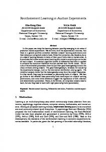
2.1.1 Robotic Paradigms A robot is generally built of several functional and structural parts whose interaction determine its behavior. There are three commonly accepted robotic primitives forming the building blocks of behavior: sense, plan, and act [32]. Sense: This primitive groups functions that take sensor signals and produce information valuable for other functions. Plan: Functions that process sensor information or internal knowledge and generate tasks to perform are of type “plan”. Act: Functions that implement the “act” primitive typically send commands to the robot’s actuators. A fourth but not (yet) generally accepted primitive is “learn”, which is of great importance for an autonomous and intelligent robot. Based on the above three primitives, different control paradigms have been formulated that describe how behavior is organized in a robot. Common control paradigms are depicted in Figure 2.1 showing their difference in the interactions of the three basic primitives. Hierarchical Control The hierarchical paradigm uses a top-down approach to build the robot control programs. It is the oldest paradigm and is based on misleading interpretations of mental introspection, suggesting that intelligent behavior is a result of repetitive sensing, planning, and acting. Hierarchical control puts much weight on the planning primitive, which masters the others. Usually, it also means that the robot has a global world model combining sensed information and predefined assumptions about the environment. From such a global world model planning derives the necessary information to generate according actions or entire action sequences. In practice this often resulted in complex algorithms with considerable computational costs. The problem faced in almost any real world application of autonomous robots is that the environment is dynamic. Changes that are not a consequence of the robot’s actions lead to the “frame problem” and the closed world assumption (all information relevant to a decision is available) does not hold. More and more it

2.1 Autonomous Robotics

5

a. SENSE

PLAN

ACT

b. PLAN

SENSE

ACT

c. PLAN

SENSE

ACT

Figure 2.1: Three robotic control paradigms a. hierarchical, b. reactive and c. hybrid deliberative/reactive1 . became recognized that an autonomous robot has to cope with uncertainty and only partial observability. To achieve this the robot must be able to adapt to changes in the environment. Reactive Control The reactive paradigm emerged to contrast the hierarchical paradigm and it builds upon low-level control loops instead of a strict control hierarchy. This paradigm is greatly inspired by biological models like reflexive behavior or stimulus-response behavior. According to these models the primitive of planning is abandoned. Control programs are organized in couples of sense-act primitives, in this context simply called behaviors. Every behavior directly links sensed information and commands for actuators. A robot’s complex behavior is achieved by running several behaviors concurrently. A sensor’s information (percept) can serve as input for one or more behaviors, and a behavior can also use percepts of more than one sensor. For the latter sensor fusion has to be done, producing one percept from several others. Since different behaviors can produce output for the same actuator, some mechanism is required to combine them in a single actuator command. Behavior based robotics [3] is heavily based on the reactive control paradigm. 1

adopted from [32], page 7

6


In this context the subsumption architecture [10] was defined, which decomposes intelligent behavior into behavioral modules. These modules are usually organized into layers that implement a particular goal of the agent. The goals of higher layers are increasingly more abstract and each layer’s goal subsumes those of the underlying layers. A big advantage of the reactive paradigm is the fast execution due to the behaviors’ limited complexity. Using this paradigm some interesting results were obtained with machines successfully mimicking animal behavior. On the other hand it became obvious that for reasonably intelligent behavior some form of planning is necessary. This observation led to the definition of the following paradigm. Hybrid Control The hybrid deliberative/reactive paradigm is the paradigm that tries to bring together the advantages of the hierarchical and the reactive paradigm. A robot constructed according to this paradigm plans by decomposing a task into subtasks. In contrast to the subsumption architecture the decomposition of a task is done by the planning instance and not at design time. For the accomplishment of subtasks suitable behaviors are selected, that execute as in the reactive paradigm. This way sensor information is available to all behaviors that require it but also to the planning instance. Similar to the reactive paradigm concurrently executing behaviors require appropriate coordination for dispatching the sensed information and for the combination of actuator commands. Robot architectures developed with the hybrid deliberative/reactive paradigm often structured the control program in layers, where one behavioral function is built on top of others. The word “deliberative” in this paradigm’s name corresponds to more cognitively oriented functions such as problem solving and learning. Deliberative functionality usually comprises modules like Sequencer determining the timed activation of behaviors, Resource Manager allocating resources to behaviors, Cartographer maintaining a map or a world model, Mission Planner interacting with a human operator, Performance Monitor and Problem Solver noticing progress and trying alternatives. The majority of todays robots constructed for complex tasks follow the hybrid paradigm [32]. Numerous different architectures are in use, each more or less specialized on some kinds of tasks. A tendency observable in many robotic projects is the growing importance of the robots interaction with humans through communication as well as social behavior [36].

2.1 Autonomous Robotics

7

2.1.2 Control Algorithms Taking a closer look on the implementation of robotic behavior in computer programs we can identify a small number of used techniques. We refer to them as control algorithms, capable of representing of low-level behaviors as well as higherlevel behavioral functionality. The used algorithms can be divided according to the underlying method of information processing.

Boolean Logic The implementation of a control program by a conventional computer program uses expressions of first order logic. Decision rules would look like IF (wall-contact-ahead = true) THEN turn around. Also allowing the use of arithmetic expressions a rule could look like IF (wall-distance-ahead < 0.2) THEN turn around. Furthermore, nested decision rules of this type lead to “decision trees”.

Fuzzy Logic Using fuzzy logic for control programs allows to define decision rules in less exact terms. In fuzzy control the sensor information is first transformed from usually real values to “linguistic variables” representing fuzzy sets (e. g., mapping a distance signal to categories like near and far). Inference rules operating on linguistic variables could have the form IF (wall-ahead is near) THEN turn around. Finally, the result derived from these rules is transformed back to usually real valued output signals.

Neural Networks An arbitrary mapping from input to output signals can also be expressed in terms of mathematical functions. A model in which simple functions are recombined in a structured way to build more complex functionality are artificial neural networks explained in detail in Section 2.2.2. Using an artificial neural network as control algorithm has the advantage that the behavior can be specified by representative examples instead of an exhaustive set of rules. More on this topic will follow in Section 2.5.1.

2.1.3 Evolutionary Robotics The previous description may have made clear that the construction of a control program that shows the desired behavior is a non-trivial task. Evolutionary robotics is the approach to let simulated evolution find a suitable control program [14]. Methods that use evolution to solve a computational problem are known as evolutionary algorithms.

8


Evolutionary Algorithms According to the Darwinian principle “survival of the fittest” organisms well adopted to their environment have better chances to survive and reproduce [11]. Organisms pass on their characteristics to the offspring generation by means of a biological blueprint, the DNA. During reproduction the DNA of the parent individuals is recombined forming an offspring that carries characteristics of both parents. Furthermore, random alterations to the DNA influence the individuals’ characteristics. Over the course of time and after many generations individuals showing favorable characteristics become prevailing. The concept has been transfered to computer science for solving computationally hard problems. Common applications are for example combinatorial optimization problems, for which no conventional algorithms are known or are infeasible due to their immense computational costs [17]. In an evolutionary algorithm an individual stands for a specific solution to the problem. The quality of a solution is assessed by an evaluation function or fitness function. Algorithm 2.1 shows the operational scheme of an evolutionary algorithm in pseudo-code. Similar to nature, evolution proceeds in generations and works on a population of individuals. At the beginning an initial population Algorithm 2.1 The basic scheme of an evolutionary algorithm. Generate initial population P repeat for all individual i ∈ P do Evaluate fitness F (i) end for Select fittest individuals for reproduction Produce offspring individuals by recombination Apply mutations to offspring individuals Form a new population P until end criterion reached of individuals needs to be generated, either from random sampling or with a heuristic. Then the algorithm repeats for each generation the fitness evaluation for all individuals and the creation of a new generation of offspring individuals. This algorithm is very generic in its structure and needs few adaptations for the application to a specific problem. First of all, the encoding of a solution (genotype) depends on the problem. Most commonly used are bitstring representations and an interpretation rule that forms a problem solution thereof (phenotype). Equally important is the fitness function that measures the performance of a solution. In case the decoding may produce invalid solutions they should have a bad fitness value. The operations for recombination (crossover) and mutation operate on the

2.2 Neural Computation

9

genotype. These operations can be generic when simple bitstrings are used, but they can also incorporate problem knowledge. Evolution of Robot Controllers Using an evolutionary algorithm to find a controller makes it necessary to repeatedly evaluate control programs for their performance. Since this process can be very time consuming it has either to be automatized as far as possible, or simulation is used instead [14]. Another important aspect is the representation of the control programs to be evolved. In the following we briefly look at two approaches, conventional programs, and neural networks. Evolution of Programs The memory representation of ordinary programs in terms of data structures and instructions can be treated as the genome of a control program. Well defined programming languages allow to decompose a program into nodes consisting of sub-nodes, representing the block of a control statement, or single instructions. An appropriate data structure for such a representation is a tree on which the EA’s recombination and mutation could operate. This method is known as Genetic Programming [22]. Although being an interesting approach, the encoding of solutions remains the crucial issue, because the building blocks determine the set of possible programs. Evolution of Neural Networks Neural networks are often represented as directed and weighted graphs, where the nodes correspond to neurons and the edges to their synaptic connections (Section 2.2). The functionality of the entire network can be described by the edges’ weights and the properties of the nodes. A possible encoding would be an adjacency matrix for the weights and a number specifying the node’s transfer function [13]. Other encodings determine only the topology of the network and leave the connection weights to be determined by learning algorithms, for which the parameters are evolved, too [46] [25]. This way the evolution of dynamic neurocontrollers can combine two paradigms observed in nature. The first is adaptation through evolution, which is also called learning of the species or phylogenetic learning. The second is adaptation by training, which is known as learning of the individual or ontogenetic learning.

2.2 Neural Computation Before computer science emerged as an own scientific discipline the definition of computability especially occupied mathematicians and logicians. In the twenties to forties of the 20th century scientists like Hilbert, Ackermann, Church, John von Neumann, and Turing postulated their theories on computability and described

10


according computational models [34]. The models reached from purely theoretical such as general recursive functions to more operational models like the Turing machine. Finally, the von Neumann computer architecture became established as the most common and practical model of computation, and it is the foundation of all modern computing devices. Since the beginning of natural sciences, fundamental knowledge in one discipline always had its impacts on other disciplines. The revolutionary insights into the structural and functional basics of brain gained by neurosciences heavily influenced the general concept of intelligence and computation. Simple mathematical models of brain functionality gave birth to a whole new field of research, which continuously evolved and today can be subsumed under the term neural computation. Seminal work has been done by McCulloch and Pitts, who roughly abstracted the functioning of biological neurons and formulated a computing model based on interconnected computing units [2]. Artificial neural networks (ANNs) try to model the information processing capability of biological neural networks. Besides information processing computation also requires some kind of data storage including an encoding scheme, and means for data transmission. In ANNs the data is transmitted via the links between neurons, and information is stored distributedly in the strength of the neural links. Therefore, artificial neural networks are often said to embody a connectionist model of computation. Scientific findings in neurobiology about the basic structural and functional principles in biological neurosystems continue to serve as inspirations for computer scientists and engineers, interested in solving real world problems. Moreover, the abstract models and their simulations provide experimental evidence for theoretical neuroscientists. Obviously, the interdisciplinary work of scientists in theoretical neuroscience and computer science is of great value for both fields [2], [4].

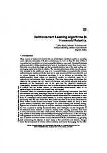
2.2.1 Biological Model The brain of higher organisms consists of a vast number of single neurons that are excessively interconnected. Here, we want to give a brief overview on the basic elements of biological neural networks to better understand their abstractions in ANNs described afterwards. Neuron A neuron, like every eucaryotic cell, is surrounded by a membrane and has a nucleus. Although in nature neurons occur in big diversity (e. g., vary in diameter from 4 to 100µm), some general characteristic structures have been identified. The body of nerve cells is called soma, that typically extends in a number of branches called dendrites. One special branch can be identified as axon, starting


11

at the axonal hillock of the cell body and an arborization at the end. The terminal points of an axon are made up of synapses, by which a neuron connects to another. The microscopic image of Figure 2.2 shows two neurons and their branches and interconnections. A more schematic illustration of a neuron and its connection to other neurons is given in Figure 2.3. Presynaptic Neuron Soma Axon Hillock Dendrites Nucleus Synapses

Axon

Nucleus

Soma

Postsynaptic Neuron

Figure 2.2: A microscopic image of two neurons1 .

Figure 2.3: A schematic drawing of two connected neurons2 .

The cell membrane’s function is to separate inside from outside, but it shows a certain permeability for different ions. Typically the concentration of sodium ions is much higher outside and that of potassium ions is much higher inside the cell. The different ion concentrations lead to a negative electric potential on the inside, which is called membrane potential or resting potential and has been measured to be about −70mV . In order to maintain this potential gradient between inside and outside ion pumps expel sodium and absorb potassium. This process consumes the major amount of energy in the neuron’s metabolism. There are ion channels embedded in the membrane with selective ion conductance, which are influenced by the presence of certain molecules. Ion channels also rapidly change their conductivity when they are excited by nearby changes in potential. This mechanism electric signals allows action potential s to propagate down a dendrite or axon. These impulses are shaped as shown in Figure 2.4 and reach up to voltage of +40mV . Continuous excitation of a neuron produce spike trains, where the spikes’ frequency corresponds to the excitation strength. 1 2

taken from http://www.pjcj.net/yapc/yapc-eu-2005-surespell/slides/index.html adopted from http://shermanlab.uchicago.edu/shopping.html

12

Chapter 2 Background +40mV

Synapse

action potential

resting potential −70mV

' .5ms ' 4.4ms

Figure 2.4: Diagram of a neuron’s action potential3 .

Axon Vesicles Synaptic cleft

Neurotransmitter

Dendrite Receptors

Figure 2.5: A schematic drawing of a synapse4 .

Synapse Signal transfer from one neuron to the next involves highly sophisticated biochemical mechanisms in the synapses. A schematic drawing of a synapse and its function is shown in Figure 2.5. The terminal buttons of the axonal branches are docked to dendrites of other neurons and contain vesicles filled with neurotransmitters. Arriving action potentials cause the vesicles to merge with the membrane, and spill their content into the synaptic cleft. The neurotransmitters diffuse to the dendrite and attach to corresponding receptors temporarily influencing the ion conductance of the post-synaptic neuron’s membrane. Many different neurotransmitters are known and are often specific to some kind of neurons. The receptors can have excitatory or inhibitory influence on the generation of an action potential in the post-synaptic neuron. The post-synaptic neuron integrates the input signals arriving from presynaptic neurons and generates new action potentials. It has been observed that the coincidence of a presynaptic and postsynaptic excitation led to a strengthening of a synaptic connection. This was one of the first indications on how learning is achieved in biological neural networks. Today, more mechanisms of neural plasticity are known that are responsible for short-term and long-term adaptations according to the neuron’s activation [1], [37].

2.2.2 Artificial Neural Networks Artificial neural networks are mathematical models abstracted from their examples in nature. Over time many different models of neural networks have been 3 4

atopted from http://hyperphysics.phy-astr.gsu.edu/hbase/biology/actpot.html adopted from http://shp.by.ru/spravka/neurosci/


13

proposed. Some of them emphasize similarities with biological neural networks while others addressed the needs of solving practical problems. The models mostly differ in two aspects. First, the functionality embodied by a single neuron and second, the networks topology determined by the connection structure. Neuron Models In analogy to biological neurons an artificial neuron has weighted connections to other neurons. The neuron sums up its input signals and produces an output signal. Put in a mathematical form, a neuron k can be described by the following two equations: vk =

m X

(2.1)

wk,j xj + bk

j=1

and yk = ϕ(vk )

(2.2)

where x1 , x2 , ..., xm are the input signals; wk,1 , wk,2 , ..., wk,m are the synaptic weights; bk is the neuron’s bias; and ϕ(·) is the neuron’s transfer function or activation function [15]. Figure 2.6 depicts a drawing of a neuron, and Figure 2.7 shows graphs of typical activation functions. x1

wk,1

x2

wk,2

1

vk

input signals

xm

Σ

ϕ(·)

bias bk

activation function

wk,m

output yk

synaptic weights

Figure 2.6: An artificial neuron5 .

0.75

0.5

0.25 threshold piecewise linear logistic sigmoid

0 -4

-2

0

2

4

Figure 2.7: The graphs of three activation functions.

McCulloch-Pitts Neuron The first neuron model developed by McCulloch-Pitts [28] was limited to binary output values {1, 0} by the use of a threshold activation function. Connections in networks of McCulloch-Pitts neurons can be either excitatory or inhibitory reflected in weights of +1 or −1, respectively [34]. By setting the threshold and the weights appopriately this kind of neuron can mimic the function of logic gates, such as OR, or AN D. 5

adopted from [15], page 11.

14


Perceptron The above basic model of neural computing was generalized by Rosenblatt [35] and others [44], [9] giving birth to the Perceptron model. The perceptron network uses real valued connection weights and has linear activation functions. The computational properties of a single perceptron neuron have been analyzed in detail, showing that only classes of linearly separable input patterns can be distinguished [29]. Topology General networks of neurons are often viewed as directed graphs where the computing units are the nodes and the weighted edges represent their connections. Feed-Forward Networks In feed-forward networks signals are processed in forward direction only. Networks of perceptrons are therefore structured in layers, where neurons of one layer are connected to all neurons of the next layer. These networks are also called multi-layer perceptrons (MLPs) consisting of an input layer, one or more hidden layers, and an output layer. Usually the activation function is nonlinear. Learning algorithms additionally need the activation function to be differentiable. The most commonly used function is the logistic function ϕ(v) =

1 . 1 + e−av

(2.3)

This fnuction also called sigmoid function due to its S-shaped curve, whose steepness is determined by the parameter a. The computational power of an MLP is supported by the Universal Approximation Theorem. Briefly summarized it says that an MLP with one hidden layer and non-linear activation function can approximate any arbitrary input-output mapping [15]. Recurrent Networks Networks, which have cycles in their connections need to define a sequence in which the nodes are updated. The neurons output is then repeatedly updated until the network stabilizes. Recurrent networks have been used successfully for the processing of temporal data (e. g., time series, and speech) and the reconstruction of complete information from corrupted data by an associative memory. To name two representatives, there are the Hopfield networks [18] and Elman networks [12] that use recurrent connections.

2.2.3 Training and Learning Neural networks are only of use when the performed mapping is well adopted to the particular application. Beside choosing a topology adapting a network to a


15

specific task mainly means determining the connection weights. In analogy to biology this process is called training or learning. The training methods for neural networks are traditionally grouped in two categories: supervised and unsupervised learning. A third method would be reinforcement learning, which is described separately in Section 2.3. In unsupervised learning the network clusters the sample data, modeling the data’s characteristics. An example of a network using unsupervised learning is the Self-Organizing Map (SOM) [21]. Training in such networks is competitive, which means that the neuron showing the highest activation for a specific sample pattern, the winner, has its input links strengthened in such a way that it is likely to fire for other similar samples. Supervised learning assumes that examples of correct input-output patterns are given. In such a case finding the appropriate weight values is an optimization problem. The error between desired output and actual network output is to be minimized, and the search space is formed by the connection weights. Since finding the weight values is an NP-complete problem, no conventional algorithm for the computation of the network’s weights exists. Instead a number of iterative methods are known to approximate good weight values. In the following two important representatives for these methods are described. Hebbian Learning The first learning rule motivated by observations made in biological neural networks is the already mentioned Hebbian learning rule [16]. Basically, it states that the connection of simultaneously active neurons should be strengthened. This rule has been formalized and applied in several variations to recurrent networks. Associative networks use Hebbian learning for the adoption of network weights. Such networks consist of two layers which are connected in both directions. The neurons use an activation function ( 1 if v ≥ 0 f (v) = −1 if v ≤ 0 which gives the neurons a bipolar encoding. After feeding an input pattern to the net its dynamics starts working until it settles at a fixpoint. The networks weights are represented by a matrix W = [wi,j ]n×k , where n is the number of input neurons x and k the number of output neurons y. When learning a specific input-output pattern the input and output values are set to the neurons and the weights are updated by ∆wi,j = γxi yj where γ is the learning constant. Applying this Hebbian learn rule repeatedly for all input-output patterns makes the network weights learn the mapping of input to output data [34].

16


Error Back-propagation For layered feed-forward networks other learning methods have been defined. The most prominent and commonly used learning algorithm is error back-propagation. Its basic idea is to iteratively minimize the networks error with respect to the desired output by performing a gradient descent in the weight space. For a more detailed explanation of the algorithm we refer to a multi-layer perceptron as shown in Figure 2.8, consisting of three layers that are fully connected.

input signal x

i

input layer

j

wk,j

hidden layer

k

output signal y

output layer

Figure 2.8: Architecture of an MLP. The connection from neuron i to neuron j has real valued weight wj,i and the output of neuron j is defined as yj = ϕ(vj ),

vj =

X

wj,i yi + bj .

(2.4)

i∈I

For the network’s training we use an error function E expressing the difference between desired output d and actual output y 1X 2 E= e , ek = dk − yk , (2.5) 2 k∈O k O being the set of output neurons. This error is called instantaneous error because it is calculated with respect to a single sample of desired input and output values. The complete learning process involves a number of different samples, but for now we look only at one of them. Performing a learning step for each sample is is called sequential mode, whereas making a learning step for all samples is called batch mode. The error is a function of the network’s independent parameters, the connection weights. The change applied to a weight is definded by th delta rule ∂E ∆wj,i = −η , (2.6) ∂wj,i


17

where η is the learn rate or step size. The negative sign of the term indicates the gradient descent, meaning that the weights are adjusted in a way to minimize the error E. Extending and transforming this formula yields (after some steps) ∆wj,i = −ηδj yj

(2.7)

using the generalized error term δ, which is different for hidden and output neurons. For output neurons it is δk = ϕ0 (vk )ek ,

(2.8)

whereas for hidden neurons it is δj = ϕ0 (vj )

X

δk wk,j .

(2.9)

k∈O

The generalized error term for output neurons uses the actual difference between desired and actual output ek . For hidden neurons the generalized error term is composed of the weighted error of all connected output neurons using the corresponding connection weights. Hence, the error is propagated backwards, from the output neurons to the hidden neurons. For the computation of the weight changes it is necessary that the neuron’s activation function ϕ is differentiable. The logistic function (see Equation 2.3) has this property and its derivation may be efficiently computed using ϕ0 (vj ) = ayj (1 − yj ).

(2.10)

From above description it can be seen that the weight adaptation process consists of two steps. First, the forward step, where the input is fed to the input neurons and the network’s output is computed. In the second step the error is calculated, which is then propagated backwards through the net yielding the necessary weight changes. To minimize the error over all given training patterns the weight adaptation has to be performed repeatedly for each of them. Although for the general case the convergence could not be shown analytically, it yields reasonable results for many practical applications. The back-propagation algorithm is widely used, but for complex problems the learning process can take quite long. Usually, the learning process is terminated when either the error signal or the weight changes reach sufficiently small values [15]. Note that the gradient descent on the error surface does not necessarily reach the global but only a local minimum. Because of the slow convergence of the standard back-propagation algorithm, several improvements have been proposed. The idea of exploiting the gradient information maximally led to the introduction of a momentum term. By doing so

18


the weight change is adjusted to the steepness of the error surface, which leads to faster convergence. Another idea is to have different learn rates for each weight and adapt them automatically to the error gradient. A variant called RPROP is based on the idea to use only the gradient’s direction and use a fixed step size depending on a weight-specific learn rate. Finally, there are algorithms like Quickprop, that take second order information of the error gradient into account. Although these improvements speed up the network training, care has to be taken in the selection of the different methods’ parameters [34]. It should be noted that no evidence has been found that error back-propagation also happens in biological neural networks. After all there is a method called constrastive Hebb learning [31], which is close to what has been observed in nature. It works for recurrent networks, and it has been shown that under certain conditions it is equivalent to back-propagation [45], [30].

2.3 Reinforcement Learning Reinforcement learning is a computational approach to learning from interaction [40]. Clearly, this kind of learning is omnipresent in human and animal behavior. From interaction with the environment animals and humans learn to adjust their behavior to a prevailing situation. This process is also captured by Thorndike’s law of effect [43]. In short it says that an animal is more likely to repeat behavior that led to a satisfying situation and less likely to repeat behavior that led to an unpleasing situation. Although a lot of animal behavior is innate, it gets adopted by an individual’s experience. An example would be a gazelle calf struggling to its feet right after birth and is able to run at high speed shortly later. Human’s neurophysiology shows an enormous individual learning capacity that enabled the emergence of a number of motional, cognitive, and social skills. A man visiting a pub to meet his friends would be an example that requires complex behavioral patterns. It means to navigate in a dynamic environment to reach the table, communicate via gestures or speech to order a drink, and associate with his mates appropriately, just to mention a few. The idea behind reinforcement learning is to make a machine learn from its direct interaction with environment. It is interesting to note that reinforcement learning is an accepted model of classic conditioning as described by the behavioral scientist Ivan Pavlov [38]. Reinforcement learning differs greatly from supervised learning, where an external teacher provides exact feedback on what the systems output should be. Instead a reinforcement learning system learns solely based on a scalar reward signal what output is good or bad. Therefore, it is said to learn from trial and error. The overall performance of a reinforcement learning system depends on how

2.3 Reinforcement Learning

19

it manages to balance between exploration (trying new things) and exploitation (making best use of past experience).

2.3.1 Reinforcement Learning Model The standard model of reinforcement learning can be characterized as follows. An agent, be it a software program or a robot, embedded in an environment has an intrinsic goal it wants to reach. As depicted in Figure 2.9, the environment’s

Environment

action (a)

reward (r)

state (s)

Agent policy (π)

Figure 2.9: The standard reinforcement learning model. state is perceived and actions are taken according to a policy. The actions taken by the agent influence the environment, resulting in a numerical reward for the agent mediating the attainment of the goal. For deciding which action to take in a certain situation the agent can use an internal value function, which serves to predict the expected reward. An agent trying to maximize the overall reward has to learn from its environment by adapting the value function. Optionally an agent may incorporate a model of the environment helping it to perform some kind of planning. Reinforcement learning is usually formulated as an optimization problem with the objective of finding a strategy for producing actions that are somehow optimal. In practice agents usually are trained on-line, which means that their policy is continuously improved while being active [5]. The mathematical formulation of reinforcement learning is based on the well elaborated theory of Markov decision processes (MDPs).

2.3.2 Markov Decision Process A Markov decision process is a decision process that deals with a stochastic environment for which the Markov property holds, each decision yields some reward

20


and the decision process has to maximize the overall reward. Markov chains describe systems by means of states and probabilities for state transitions occurring at discrete time steps. A system has Markov property if the probability of being in a specific state exclusively depends on its direct predecessor state. For a system described by such a Markov chain an optimal decision policy can be defined. A policy consists of a sequence of decisions and the definition of optimality depends on the temporal extension of the decision process. Due to the process’ stochastic nature the optimality is based upon the expected value of the overall reward. In case that there are defined terminal states that have to be reached the decision process has a finite horizon, otherwise it has an infinite horizon [15]. According to Bellman’s optimality principle an optimal policy always includes an optimal decision sub-sequence. Based on this principle an optimal policy can be constructed from back to forth. This generic method for solving optimization problems is called dynamic programming [7]. It was originally described by Bellman in the 1950s and over time it evolved to a scientific field of its own.

2.3.3 Optimal Control Assuming that we have a Markov model of the environment, the optimality principle allows us to construct an optimal decision policy by an iterative process. As described in the learning model above the result of an agent’s decision or action is a state transition st → st+1 and a reward rt+1 . The state transition probability from state s to state s0 is denoted by Pss0 . The reward in time step t + 1 can be expressed as a function of the previous state st and the agents action at . Rewards are like state transitions stochastic for which E indicates an expected value in the following equation. E[rt+1 |st , at ] = R(st , at )

(2.11)

The evaluation of a policy V π over the entire decision process starting in state s can be expressed by a weighted sum over all (future) rewards. ·X K ¯ h i V π (s) = Eπ Rt ¯¯ st = s = Eπ γ k rt+k+1

¯ ¸ ¯ ¯ st = s ¯

(2.12)

k=0

By restricting the weighting factor γ to a value in the range (0, 1) later rewards are weighted less than earlier ones limiting the influence of long-term consequences. Additionally this ensures that the sum is finite even if the decision process’ horizon K is infinite. Using this definition we can say that a policy π is optimal, if no other policy 0 0 0 π is better in the sense that V π (s) ≥ V π (s) for all states s and V π (s) > V π (s) for at least one state. The optimal policy is denoted as π ∗ and the corresponding optimal value function as V ∗ .

2.3 Reinforcement Learning

21

2.3.4 Value Iteration Assuming a fixed policy, the value function can be computed by successive approximations. By Vn∗ (s) we denote the optimal value function for the first n steps when starting in the state x. This evaluation function represents the maximal expected reward signal. We start by computing the optimal value function only for the first step. V1∗ (s) = max R(s, a) (2.13) a∈A

Now we iteratively compute the optimal value function for more steps. A value function for n steps uses the discounted evaluation function of a previous step n − 1, having γ as discount factor. ·

Vn∗ (s) = max R(s, a) + γ a∈A

X

¸ ∗ Pss0 (a)Vn−1 (s0 )

(2.14)

s0 ∈S

By successively increasing the number of steps taken into account the value function Vn∗ approximates the optimal evaluation function V ∗ . For this evaluation function the only optimal policy is the greedy policy, which chooses the action with the highest expected reward. Formally the chosen action maximizes the expression R(s, a) + γ

X

Pss0 (a)V ∗ (s0 )

(2.15)

s0 ∈S

If no complete model of the decision task is available the value function cannot be computed but it has to be estimated [6]. A method to continuously approximate the value function while interacting with the environment is temporal difference learning, described in Section 2.4.

2.3.5 Policy Iteration Another method to find an optimal policy would be to continuously improve the policy itself. The expected return of a policy π defined above as V π allows to compare two policies. Changing from one policy π to another π 0 does not require to compute V for both. Instead, the expected return for this composite policy is R(s, π 0 (s)) + γ

X

Pss0 (π(s0 ))V π (s0 ).

(2.16)

s0 ∈S

A new policy π 0 can be constructed that maximizes the immediate expected reward R(s, π 0 (s)), which is provably better with respect to the expected reward V . This means that we can start out with an arbitrary policy and successively adjust it whenever a better one is encountered and stop if no better policy can be found. Within the process of forming new policies the corresponding evaluation

22


functions are computed. It is guaranteed that this process will produce an optimal policy after a finite number of iterations [6]. Methods for estimating optimal policies in the absence of complete models of the decision task are known as adaptive or learning methods. Other methods for directly searching in huge space of possible policies would be evolutionary algorithms, or simulated annealing [15].

2.4 Temporal Difference Learning Temporal Difference learning (TD) was introduced by Sutton [39] and comprises a set of methods that solve the reinforcement learning problem. Basically, these methods use the difference of the value function in two subsequent time steps to update the evaluation function. TD combines good properties of two other methods. It is related to dynamic programming techniques because it successively improves its estimate based on previous estimates. This property makes is especially useful to start from scratch, which is known as bootstrapping. Moreover, it is similar to Monte Carlo methods because it learns by sampling the environment according to some scheme. The term “Monte Carlo” in a broader sense often refers to an estimation method that makes use of random elements. In the context of a stochastic environment we mean a method that averages over a number of trials with a specific policy and an estimated value function before updating the later. In the previous sections we assumed to have a complete model of an agent’s environment by means of state-transition and payoff probabilities and to construct an evaluation function and a decision policy thereof. Unfortunately, for real worlds problems almost never such a model is available, but without a model an agent cannot evaluate actions without actually performing them. Fortunately, TD learning does not rely on a model but directly estimates an evaluation function from experience [39]. In an abstract form the incremental update rule for the evaluation function’s estimate is given by the following expression. N ewEstimate ← OldEstimate + StepSize(T arget − OldEstimate) The difference between T arget and OldEstimate is called temporal difference. For an entire learning process the agent usually has to perform a number of trial runs called episodes. In an episode the agent is put in a starting state and has to make its control decisions either until a terminal state or another end criterion is reached. Within this process updating of the evaluation function can be performed at different points in time. One possibility is to update after each control decision of the agent, which is known as on-line training. The other possibility is called

2.4 Temporal Difference Learning

23

batch training and performs the update only after each episode. In the following we discuss a few specific learning rules.

2.4.1 TD(0) The simplest temporal difference learning algorithm is called TD(0). It approximates the evaluation function according to the following equation. ³

´

V (s) ← V (s) + η r + γV (s0 ) − V (s)

(2.17)

As described previously γ is a discount factor that weights the influence of an action’s consequences and the step size η is similar to the learning rate in neural network training algorithms. The TD(0) learning algorithm is described in pseudo-code by Algorithm 2.2. Assuming that the state space S is discrete, the evaluation function V (s) can be Algorithm 2.2 The TD(0) reinforcement learning algorithm. Select a policy π Initialize V (s) arbitrarily for all episodes do Initialize s repeat a ← action given by π in state s Take action a, Observe reward r and next state s0 V (s) ← V (s) + η(r + γV (s0 ) − V (s)) s ← s0 until episode is completed end for stored in a tabular form. Whenever the agent comes to state s its estimation of the evaluation function V (s) is updated according to the temporal difference and the immediate reward r [40]. The analysis of this algorithm follows from the policy evaluation function given in Equation 2.12. From this formula an update rule can be derived, which uses the previous prediction of the current state’s value and the reward signal to update the value of the preceding state. ·

V π (s) = Eπ

·

¯ ¯

P∞

¸

k ¯ k=0 γ rt+k+1 ¯ st = s

= Eπ rt+1 + γ

P∞

¯ ¯

¯ ¸ ¯ π ¯ = Eπ rt+1 + γV (st+1 ) ¯ st = s ·

¸

k ¯ k=0 γ rt+k+2 ¯ st = s

(2.18)

24


2.4.2 SARSA The method’s name stands for State-Action-Reward-State-Action and indicates that this method considers transitions of state-action pairs. Instead of the statevalue function V π (s) used in the TD(0) algorithm an action-value function Qπ (s, a) is used. It is defined as the expected return starting in state s and taking action a under a policy π. ·X ∞ ¯ i ¯ Q (s, a) = Eπ Rt ¯ st = s, at = a = Eπ γ k rt+k+1 π

h

¯ ¸ ¯ ¯ st = s, at = a ¯

(2.19)

k=0

Based on this definition the SARSA algorithm iteratively updates its estimation of the evaluation function. ³

´

Qπ (s, a) ← Qπ (s, a) + η rt+1 + γQπ (st+1 , at+1 ) − Qπ (s, a)

(2.20)

SARSA is an on-policy method, which means that the value function is updated for the action actually performed. Q-Learning described in the next section is an off-policy method. Algorithm 2.3 shows the learning procedure in pseudo-code. Similar to the TD(0) algorithm the estimated values Q(s, a) can be stored in a Algorithm 2.3 The SARSA reinforcement learning algorithm. Initialize Q(s, a) arbitrarily for all episodes do Initialize s a ← action derived from Q in state s repeat Take action a, Observe reward r and next state s0 0 a0 ← action derived from ³ Q in state s ´ π π π Q (s, a) ← Q (s, a) + η rt+1 + γQ (st+1 , at+1 ) − Qπ (s, a) s ← s0 , a ← a0 until episode is completed end for matrix, which is successively updated. An appropriate policy that depends on the estimated values is the ²-greedy policy. This policy in most cases selects the action with the highest estimated Q-value, but with a certain probability ² it selects a random action. Thereby, this policy accounts for exploitation as well as for exploration. It has been shown that Q approximates the optimal action-value function Q∗ , if the repeated training of all episodes ensures that all states are visited an infinite number of times [40].

2.5 Neurocontrollers with Reinforcement Learning

25

2.4.3 Q-Learning Q-Learning is similar to SARSA as it approximates the action-value function, but it uses a fixed policy. This has a significant advantage for the formal analysis of the algorithm and allowed to proof that Q converges to the optimal action-value function Q∗ . The update rule used in Q-Learning calculates the temporal difference based on the action with the highest value, independently of what action is chosen by the policy. Therefore, it is called an off-policy method of reinforcement learning. ³

´

Qπ (s, a) ← Qπ (s, a) + η rt+1 + γ max Qπ (st+1 , a) − Qπ (s, a) b a∈A

(2.21)

Generally any policy can be used, if only it remains fixed for the entire learning process. The Q-Learning algorithm is very similar to SARSA, with the only difference in the update rule [40].

2.5 Neurocontrollers with Reinforcement Learning The construction of a controller steering a robot has to take the dynamics of the robot’s environment into account. According to control theory, which is an established field that deals with the behavior of dynamic systems, a controller manipulates a system’s input to obtain a certain output. Control loops make use of the system’s output by forming a feedback signal from it to adjust the input. Considering the controller of an autonomous robot, its actions can influence the environment or the way it is perceived in the future.

2.5.1 Neural Robot Control One approach to construct a robot’s controller is to define its behavior by means of decision rules, mapping sensory input to actuator outputs. As described earlier (Section 2.2.2) ANNs are able to learn arbitrary input-output mappings. Usually MLPs are trained by an algorithm on the basis of desired input-output patterns. For autonomous robots such an example based approach is problematic. First, examples for the desired robot behavior have to be provided. Furthermore, these examples have to be good representatives of all possible situations the robot could encounter. A solution already discussed (Section 2.1.3) would be the evolution of an appropriate neural net. Another way to overcome this problem is to use reinforcement learning. For the application of reinforcement learning it is enough to provide some positive reward for wanted situations or negative reward for unwanted situations. Training a neural network that represents an approximate value function takes advantage of the ANN’s generalization capability. This means that the training

26


does not necessarily include all possible states or input patterns, but the network abstracts from examples. A fact that is particularly useful when the input consists of real values, making exhaustive sampling impossible. It is a particular strength of reinforcement learning methods, that they are able to produce meaningful behavior based on sparse or delayed reward signals. The method of combining reinforcement learning with neural networks is known as Neuro-Dynamic Programming (NDP) [8]. In their equally named book Bertsekas and Tsitsiklis gave the following definition. Neurodynamic programming enables a system to learn how to make good decisions by observing its own behavior and to improve its actions by using a built-in mechanism through reinforcement. In this context “observing their own behavior” means the use of simulation, and “improving their actions through a reinforcement mechanisms” means an iterative process to approximate the optimal value function in order to obtain the desired behavior.

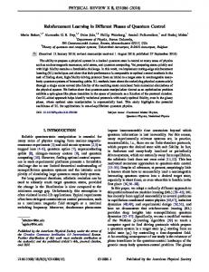
2.5.2 Temporal Difference Control For our robotic learning experiments we chose an on-line training method that is able to bootstrap. A suitable TD learning method is Q-Learning, for which the evaluation function for state-action pairs is implemented by a neural net [41]. The robot’s state is directly derived from the current sensor signals, whereas the actions consist of possible signals for the actuators [33]. For the generation of output signals several methods have been proposed. Possibilities are to use either a fixed set of predefined actions, or a set of randomly generated actions. Additionally, a “creative network” could be used to generate novel actions based on past experience [24]. The operational scheme of a temporal difference neurocontroller is depicted in Figure 2.10. The controller periodically performs a control decision. For each z −1

reward (r) TD(0)

action (a)

state (s) Neural Net

Q(s, a) policy (π)

Actions

Figure 2.10: The TD neurocontroller.

2.5 Neurocontrollers with Reinforcement Learning

27

control decision the state is read from the sensors and then together with each of the possible actions is fed to the neural net for evaluation (Q(s, a)). The robot usually takes the action action promising the highest reward (²-greedy policy), but with a certain probability ² this policy selects a random action. In general the neural net is only a approximation of the optimal value function, which means that other actions may yield higher reward than the network “expects” [40]. Hence, the random factor in the action selection policy accounts for the exploration of unknown states and actions. After each control decision the neural network is trained using the reward signal and temporal difference of the network’s evaluations. This way the evaluation of the preceding action is corrected, performing the temporal credit assignment. The neural network is trained with the back-propagation algorithm using the temporal difference value as an error signal. Thereby the networks weights are adapted in order to improve the evaluation, accounting for the structural credit assignment [42], [39]. Formally, this learning step can be expressed by the following equation. h

i

w ~ t+1 = w ~ t + η rt+1 + γQt+1 − Qt ∇w~ t Vt

(2.22)

The vector w ~ stands for the network weights, which are adjusted according to the gradient of the value function.

29

Chapter 3 Robot Simulator The simulator used for our experiments is called SiMMA, which is an acronym for Simulator for EMMA. It is a lean, modular, and flexible simulation framework allowing to simulate a wide variety of scenarios. This software package has initially been written by a group of students as a seminar project and is continuously extended by those using it for their master thesis or research.

3.1 Design Throughout the development of the simulator great importance was given to extensibility and ease of use. Therefore, SiMMA has been built as a framework implemented in JAVA according to our requirements.

3.1.1 Features The simulator’s basic concepts and characteristics can be described as follows: modularity Any kind of object can be simulated, once its properties and behavior have been implemented in a simulation entity. Such a simulation entity can be composed of sub-entities and define their interactions. discrete time The simulation is performed in discrete time steps, where the step size is configurable. The simulation time can either proceed in real time or in virtual time running as fast as possible. In each time step all simulated objects are updated sequentially. environment The physical world in which the entities are simulated is a twodimensional euclidean space, e. g., a plane. physics Physical properties such as position, velocity, mass, and shape are handled by the simulation. The simulation environment also cares for basic collision handling.

30

Chapter 3 Robot Simulator

Figure 3.1: A static view of SiMMA’s framework classes. reporting For the evaluation of experiments running in the simulator a reporter is engaged, which collects and records the appropriate information, e. g., to files. run mode The simulator has two different operation modes. In interactive mode it shows a visualization of the simulation scenario allowing a user to interactively control the simulation. In batch mode the simulation runs without visualization, which allows for fast computation of a lager number of experiments.

3.1.2 Software Structure The core parts of SiMMA are laid out in a very generic way in order to keep the program modular and easily extensible. Hence, these parts constitute a simulation framework, which is illustrated by the class diagram in Figure 3.1. The application’s entry point is the class Simma forming also the heart of the simulation. This class keeps a list of simulation entities (SimmaObjects), which are periodically triggered to update their own states. Furthermore, Simma can use a Reporter, which is regularly updated and records the simulation. The optional visualization is encapsulated in the class SimmaView, which utilizes SimmaObjectViews provided by the simulation entities to draw a screen representation of them. Every simulation entity can be composed of several parts, each represented by another SimmaObject. The framework’s class AbstractRobot models a generic robot consisting of a number of sensors, actuators, and a controller linking them together. A generic sensor which supports the characteristic operation getSensorValue() is represented by the class AbstractSensor. Similarly, the class AbstractActuator rep-

3.1 Design

31

Figure 3.2: Control flow of a simulation step. resents a generic actuator supporting the characteristic operation setActuatorValue(value). The class AbstractController stands for a generic controller that is periodically triggered to perform its control decisions.

3.1.3 Flow of Control and Information Most importantly, the framework also defines a certain flow of control. The timing of the simulation is performed by the SimulationTimeManager class, which maintains also the simulation’s logical clock. It is responsible for the execution speed by triggering the computation of each simulation step. Updating the simulation is done in two phases. First the update() method of all SimmaObjects is called and then possibly occurred collisions between the objects are resolved. Each SimmaObject is responsible to update all its sub-entities it is composed of. Resolving collisions relies particularly on the implementation of the SimmaObjects. Whenever Simma detects that two objects may have collided they are informed to deal with it appropriately. For the simple cases where two round objects collide or a round object hits a wall, libraries offer functions to separate the objects appropriately. For the simulation of a robot with all its equipment the framework defines a clear model of interaction. Sensors and actuators implement the respective interfaces (ISensor, IActuator) and are addressed thereby. A controller may read the input values via the the robot by calling getSensorValue(name) and set the output values by calling setActuatorValue(name,value). The names of the sensors and actuators that the controller may use to address them are determined by the configuration. Figure 3.2 shows this procedure in a sequence diagram.

32


Figure 3.3: A screenshot of SiMMA running a wall avoidance experiment.

3.2 Simulator Usage For a specific simulation scenario the framework described above has to be extended by the implementation of concrete classes. For our task we implemented classes representing the robot including all its equipment and the robot’s arena. A visual impression of how a simulation looks like on SiMMA’s graphical user interface is given by Figure 3.3.

3.2.1 Configuration Running a simulation with the appropriate classes requires a certain configurability of the framework. The configuration for an experiment is contained in an XML file. Basically, a SimmaObject corresponds to every XML element in the file, and its sub-elements correspond to the SimmaObject’s equipment. On startup SiMMA instantiates the SimmaObjects from the class names specified in the class attribute of the according element. Additionally, the configuration contains general settings like the duration of a simulation time step, parameters for the reporter, the operation mode, and respective parameters. An example of such an experiment configuration can be found in Appendix A.1.2. At runtime the composition of objects is determined by the configuration describing the experiment setup. The classes involved in a wall avoidance experiment and their relations are depicted in Figure 3.4. RectangularArena The arena where experimenting with EMMA2 takes place is

3.2 Simulator Usage

33

Figure 3.4: A class diagram of a simulation experiment (without visualization). represented by the class RectangularArena, which has configurable width and height. Emma In Emma we modeled the real robot EMMA2 as described in Chapter 4. In this example it’s equipment is configured with the number and type of sensors and actuators used in our wall avoidance experiment. BumperSensor The class BumperSensor simulates the real robot’s wall contact sensor. DistanceSensor The class DistanceSensor mimics the infrared sensor device and its characteristics as used in EMMA2 (Section 4.1.3). NeuroController Cotrollers using neural nets are generalized in the class NeuroController which can have several “brain areas”. The simulation of neural networks is accomplished by a separate software package called Boone [23]. TDController This class is a special type of NeuroController using the temporal difference learning algorithm described in Section 2.4 and its application to robot control in Section 2.5.2. Its implementation is described in more detail in the following section.

34


TwoWheelDrive The actual drive of EMMA2 with two independently controllable wheels is represented by class TwoWheelDrive having configurable wheel spacing and diameter. WallAvoidanceReporter The recording of our learning experiments is done by the class WallAvoidanceReporter. This reporter amongst other things logs the time the robot has wall contact and the path traveled by the robot. The logged data is written as comma separated values to CSV files in the configured directory. The name of the observed robot and the rate at which the logging is performed are also taken from the configuration. In addition to reporting this class also performs the sequencing of learning experiments. To trigger the different phases of the experiment it makes use of the SimulationTimeManager. The number of experiments and duration of the experiments’s phases are specified in the configuration. All the software models of physical entities (e. g., sensors and actuators) have been continuously refined to make the simulation as realistic as possible.

3.2.2 Temporal Difference Neurocontroller For our learning experiments the most crucial part is the neurocontroller making use of the temporal difference learning algorithm (Section 2.4). The simulation of artificial neural networks is accomplished by a dedicated software package called Boone, which stands for Basic Object-Oriented Neural Environment [23]. In contrast to a conventional neurocontroller, that maps sensor outputs to actuator inputs, the temporal difference algorithm demands a different net structure (Section 2.5.2). Here, the neural net maps state-action pairs to a single output, that represents an assessment of an action in the given state. The robot’s state at a certain moment is described by the signals from the sensors, and an action is composed of potential signals for the actuators. The basic operational scheme of the TDController consists of two parts, one is the actual control decision and the second is for the learning. 1. control a) b) c) d)

read state, St generate actions, A˘t = {Ait , i = 1..n} net computes values of all actions, V (St , a), a ∈ A˘t select action with highest value, At = arg max V (St , a) ˘t a∈A

e) set action and record its value, Qt = V (St , At ) 2. learn a) calculate the temporal difference of values, Qt − Qt−1 b) use this difference and the reward to train the net with the previous state and action

3.2 Simulator Usage

35 front distance right distance

state

back distance left distance

value

bumper right wheel

action left wheel

Figure 3.5: Neural network layout for learning the wall avoidance task by temporal difference. state The sensor signals reflecting the robot’s state come from the wall contact sensor and four distance sensors. Naturally the wall contact sensor supplies a binary value {0, 1}, whereas the distance sensors yield continuous values in the range of [0, 1]. action Two speed values for the left and the right motor control the robot’s action. We chose to use a fixed set of actions that consists of the 25 pairs that make each wheel go at one of the 5 following speeds: full backward, half backward, stop, half forward, full forward, encoded by the numerical values 0, 0.25, 0.5, 0.75, 1, respectively. net The state-action pair is represented by 7 values and the neural net has the according number of input neurons. Using one hidden layer the net’s layout looks as depicted in Figure 3.5. The hidden neurons have the common sigmoidal activation function, but the output neuron’s uses the identity function. policy The selection of one of the possible actions is based on a specific policy. We use an ²-greedy policy, which does not always choose the action with the highest value, but with a certain probability (² = 0.01) chooses a random action. This technique makes the algorithm try out actions different from the one with highest value, and by that explore the space of state-action pairs. reward The on-line training of the neural net makes use of an external reward to direct the learning of the value function. In our case the reward is directly derived from a sensory input, the wall contact sensor. When the robot hits the wall,

36


a negative reward signal is produced. Thereby, the assessment for the previous action leading to the collision is adjusted. learning The neural network is trained with the back-propagation algorithm using the temporal difference to adapt the net’s weights. In the course of our experiments at certain moments the robot gets repositioned, causing the robot’s state to change. Whenever a state change was caused externally or a random action was chosen the network is not trained, since the temporal difference is not the result of the neurocontroller’s decision.

37

Chapter 4 Mobile Robot The robot we use for our experiments is called EMMA2, which stands for EMbedded Mobile Agent second generation. It is an autonomous, mobile, and vision enabled robot, designed and constructed in the RoboLab within a bachelors project [19]. Potential applications include experiments in evolutionary robotics and reinforcement learning.

4.1 Hardware Platform 4.1.1 Concept EMMA2 is made of two main components: a handheld computer on the one hand and a drive on the other hand. Figure 4.1 shows a conceptual drawing of the robot and Figure 4.2 a current photo of the complete robot. Using a handheld as the central computing device of the robot has several benefits. Most importantly, a lot of development and construction time was saved by using an off-the-shelf device instead of a self-made mainboard. Fortunately, the handheld already comes with a complete operating system and a suitable software development tool chain. The robot’s drive consists of a chassis, an electronic control board, two stepper motors, and two accumulator packs. The electronic control board and the handheld are connected via an infrared data link (IrDa) and use the Emma Hardware Control Protocol (EHCP) to exchange information. The firmware running on the drive’s control board mediates between the control application on the handheld and the sensors and actuators connected to the control board.

4.1.2 Control Board The drive’s electronic circuit is built of several components. First, there is a rechargeable power supply based on two accumulator packs. Each consists of 6 cells with a nominal voltage of 7.2V and a total capacity of 600mAh, which allows the robot to operate for about one hour. The accumulator’s voltage is transformed

38

Chapter 4 Mobile Robot

IrDa Communication

Handheld: Palm Zire 72s

250mm Wall Contact Sensor

Controlboard: AVR ATmega16 Distance Sensor: Sharp IR

Battery Packs: 2 x 7.2V, 600mAh Stepper Motors: 2 x ST2818S

100mm

Figure 4.1: A sketch EMMA2.

of

the

robot

Figure 4.2: A recent photo of the robot EMMA2.

by a voltage regulator to provide a constant power source of 5V for the control board. A stepper motor driver chip is powering the two connected motors. The infrared (IrDa) transceiver and the protocol stack handler chip are responsible for the data link with the handheld computer. The AVR ATmega16 microcontroller forms the heart of the control board. It runs the control board’s firmware and accepts commands from the IrDa interface in compliance with the EHCP, which specifies format and semantics of the transmitted messages [19]. Additionally, a generic analog and digital interface allows the connection of further sensors and actuators.

4.1.3 Sensors and Actuators The robot’s equipment necessary for the wall avoidance experiment are a motor drive, distance sensors and a wall contact sensor.

4.1 Hardware Platform

39

Motor Drive The robot’s central and already built-in actuator consists of two independent motors driving the left and the right wheel. When the handheld sends the appropriate EHCP commands the microcontroller’s firmware makes sure that the stepper motors are triggered accordingly. A stepper motor needs an impulse for each step of rotation and they are generated by the firmware using hardware timers. The motors rotation speed is indirectly proportional to the time between two impulses. To still achieve linear speed control, the firmware takes two numbers to determine a wheel’s speed (for details see [19]). Respecting the highest possible rate of timer interrupts the maximum speed is limited to 0.2m/s. Distance sensors The robot is equipped with four distance sensors, one heading in each direction. Each sensor element (Sharp IR GP2D12) provides an analog signal (almost) proportional to the distance. In fact the sensor characteristic is a non-monotonic function as depicted in Figure 4.3. The sensor is connected to the generic I/O interface, and the signals are then directly fed into the microcontroller. Upon request over EHCP the signals are digitalized and sent to the handheld. To record the characteristic of the sensor element its output for distances between 0 and 1m has been measured, producing values in the range of 0.4 and 2.6V . From the measured data an approximation was found using an exponential model. The resulting function looks as follows, where d is the exact distance and s is the produced output signal. (

s=

0.91 − (1.045 + d)−10 0.031 + (1.068 + d)−6.28

for d < 0.05 for d >= 0.05

Additionally to the data measured from the real sensor Figure 4.3 also shows the two models used for simulation. The one used in simulations experiments of previous work (simple logarithmic model) and the more realistic (model of hardware). Wall Contact Sensor In order to give the robot feedback upon wall contact we built another sensor which generates a signal when the robot touches the wall. Our self-made wall contact sensor is made of minimal components: two wire rings, a pull-up resistor and a connector. Figure 4.4 shows the schematic drawing of the sensors electronic circuit. As depicted the output signal of that circuit is logically inverted. The pull-up resistor provides for a high signal on the output line, necessary for the open collector input of the microcontroller. When the two

40


Sensor characteristic: Sharp IR GP2D12 1

measured from hardware model of hardware simple logarithmic model

Sensor Output

0.8

0.6

0.4

0.2

0 0

0.2

0.4 0.6 Distance [m]

0.8

1

Figure 4.3: The characteristic curve of the Sharp distance sensor. +5V

50kΩ ¬WallContact GND

Figure 4.4: The electronic circuit of the wall contact sensor. wire rings surrounding the robot’s case get in contact with a conductive surface an electric circuit is closed producing a state change from logical one to zero. By sending an appropriate request the handheld can retrieve the sensors current state.

4.1.4 Handheld The most vital part of the robot is the handheld since it runs the control application, and therefore it can be seen as the robot’s “brain”. In EMMA2 a Palm Zire 72s is put to use and its hardware has the following characteristics: • Intel XScale 312MHz ARM Processor • 32MB RAM and 16MB ROM • IrDa and Bluetooth interface

4.2 Software Environment

41

• Slot for SD-Memory cards • Video camera with 640x480pixel and microphone • TFT color display with 320x320pixel • Rechargeable battery for about 2 hours of continuous operation This computer is running an operating system (Palm OS 5.2.8) that provides a convenient basis for any additional software needed for controlling the robot.

4.2 Software Environment On top of the pre-installed operating system some more software is needed in order to integrate the handheld and the drive into the robot EMMA2. • Websphere Micro Environment (J9) is a Java virtual machine provided by IBM for Java Micro Edition (J2ME). More precisely, it implements the two standards Connected Limited Device Configuration (CLDC 1.1) and Mobile Information Device Profile (MIDP 2.0), which means support for several necessary or useful Java language features, e. g., floating point arithmetic, dynamic instantiation of classes by their name, and socket communication. • Emma Modular Control Concept (EMCC) is a framework and runtime environment for robot control applications, which has been developed in a students project in the RoboLab [20]. It is entirely written in Java and well adopted for the use in the J9 virtual machine on a Palm. • AutoOff is a tiny program that allows to overrule the automatic power off facility of the Palm OS. This power save mode is useful when the Palm works as a personal digital assistant, but does not make sense when running a robot’s control program. The following section describes the design and use of EMCC in more detail.

4.2.1 Robot Control Application The behavior of an autonomous robot is based on the three basic primitives sense, pan, and act (Section 2.1.1). The control process consists of these primitives executed in subsequent steps. 1. coordinated reading and processing of the robot’s sensor inputs 2. applying the controller logic by transforming input to output signals 3. sending these outputs to the robot’s actuators

42


Most of the controlling process is independent of the specific control task, especially steps 1) and 3), which motivates the creation of a software framework for that. EMMA Modular Control Concept (EMCC) The EMCC framework and runtime environment implements the generic parts of a robot control application, and is flexible enough to support different hardware configurations according to the demands of specific experiments. Sensors and actuators are abstracted in an object-oriented way so that each relevant hardware entity is represented by an object. Communication with the control board via EHCP is encapsulated in dedicated libraries. The framework defines initialization and termination mechanisms for control programs, and structures the interaction of control programs, actuators, and sensors. The framework provides a highly modular and easy-to-understand collection of Java interfaces and classes, which allow easy adaptation to new control tasks. This means that for creating a new robot application, the framework has to be adapted in two ways by the control engineer. First, the control logic has to be implemented in a controller. Second, a configuration file reflecting the robot’s setup has to be written. From this description as well as from its roots it can be seen that the robot control framework is closely modeled after the structure of the robot simulation in SiMMA (see Section 3.1.2). EMCC Architecture The class EMCC is the main class of the application, and since J2ME can only run so-called MIDlets, EMCC extends this class and serves as the application’s entry point. On startup it instantiates and configures the Robot object, which itself instantiates all its equipment (sensors and actuators) according to the current configuration. A class diagram of the framework is shown in Figure 4.5. The central class in the framework’s architecture is Robot, as it represents EMMA2 in its current configuration. It maintains both a set of sensors, and a set of actuators as well as a controller. Sensors and actuators represent hardware devices, such as distance sensors or motors, while a controller is a software component that processes information of sensors and controls actions of actuators. It embodies the application logic that operates the robot. The interfaces ISensor and IActuator are generic and suitable for a wide variety of different sensor and actuator types. Sensors may be considered as sources of information, while actuators are information sinks. Each specific sensor or actuator is associated with a specific type of information, e. g., a motor is controlled by a real number encoding speed, a bumper sensor provides binary


43

Figure 4.5: A class diagram of EMCC’s architecture. values, a camera yields an image, etc. For this EMCC provides the (marker) interface IValue that generalizes specific values. Control Flow The basic idea behind EMMC’s flow of control is a time-triggered controller, which has to implement a method performPeriodicAction(), which is periodically called by the TimeManager. This method is assumed to follow the well-known scheme of input-processing-output. In the input phase, the controller reads values from sensors, followed by some processing, and finally sets actuators in the output phase. This process is illustrated in the sequence diagram in Figure 4.6. The controller gets sensor values and sets actuator values via the robot. Since the robot maintains all sensors and actuators, a controller has no reference to them but “knows” them only by their name (defined in the configuration file). This makes the controller code that wires sensors, control logic, and actuators easy to read and understand. EMCC Facilities Software components representing sensors or actuators that are connected to the control board use the communication facilities of the EMCC runtime library. The communication protocol with the control board is implemented in two layers. The

44


Figure 4.6: Time triggered flow of control.

Figure 4.7: A distance sensor utilizing communication libraries.

lower layer is implemented in the class IRCommunicator, which maintains the IrDA connection and does the error handling. The upper layer, EmmaHWCommunicator, implements the actual EHCP, and provides a method for each message type of the protocol [19]. It offers higher level services such as controlLeftMotor() or readAnalogueValue(). The methods controlLeftMotor() and controlRightMotor() take a speed value (m/s) as parameter and performs the transformation into control values for the drive. The readAnalogueValue() method’s parameter specifies a pin from the control board’s generic I/O interface that should be read. In Figure 4.7 a sequence diagram depicts the process when a distance sensor utilizes the EmmaHWCommunicator to update the sensor state.


45

Configuration The configuration of the framework for a specific experiment is done via an XML file. The element tree in such a file represents the composition of the robot’s components, such as sensors, actuators, and the controller. Each of the elements representing a component must specify a class attribute, containing a fully qualified class name, necessary for object instantiation via reflection. As mentioned above, a controller only uses the names of robot equipment for interaction, which are defined in the name attribute of the corresponding tag. Components that implement IXMLConfigurable are handed their XML tag after instantiation to initialize themselves. They may use sub-elements in the XML tag for componentspecific configuration or the configuration of further sub-components. A sample configuration can be found in Appendix A.2.4. Since there is no debugging support for the J9 on the Palm, the framework comes up with a simple but nice logging facility implemented in the library class Logger. The logger, like every logging message has a verbosity level. A message sent to the logger is either written to the display when the logger’s verbosity level is higher or discarded otherwise. With further development of EMCC a RemoteLogger has been added, which sends the logging messages over a socket to a remote host. A desktop application (LoggingMonitor) able to display the messages received via a socket connection is described in Appendix A.3.2. Networking Furthermore the runtime library contains the class SocketCommunicator for simple stream based communication. This class also offers methods for type safe reading and writing of primitive data types, and does the error handling. It has proven be very useful, e. g., for a remote control (see Section A.3.1), or the experiment director (see Section A.3.3). When EMCC makes use of socket communication it relies on the networking capabilities of the Palm. Its operating system allows to connect to a network in several ways. The method we used is based on the standardized Bluetooth’s LANAccess profile and can be configured easily on the Palm. The prerequisite for this is either a Bluetooth LAN access point or a desktop computer with a Bluetooth adapter and adequately configured LAN access.

4.2.2 Temporal Difference Neurocontroller A generic neurocontroller (class NeuroController) constitutes the basis for the realization of neural control applications for the robot EMMA2. For the simulation of neural networks a separate software package called BooneMe is used. This is a version of Boone [23] that is adjusted for the use with J2ME (see Appendix A.4

46


for details). The implementation of the temporal difference control and learning algorithm follows closely the description already given for the class TDController in SiMMA in Section 3.2.2. Briefly reviewed the temporal difference controller works as follows: The neural net evaluates state-action pairs and the most promising action is taken. The network is continuously trained with the errors of its own predictions and uses external feedback to improve its evaluation function.

4.3 Remote Control In our experiments we needed to interact with the usually autonomously operating robot. Sockets available on the Palm’s Java virtual machine provide a proper basis for communication between a PC and the robot. A desktop application was built, that helps with the following tasks: • displaying log messages from the robot • testing and measuring characteristics of sensors and actuators • sequencing and reporting of a learning experiment • transferring neural nets from and to the robot These tasks are implemented in three separate components of one application. The main application acts as a server that listens to the ports of all components. When the robot establishes a connection to one of these ports, the corresponding component is started, which itself displays an appropriate graphical user interface (GUI). A detailed description of the components of this desktop application and their usage can be found in Appendix A.3.1.

47

Chapter 5 Experiments The general objective of our work is to compare the behavior of a temporal difference neurocontroller in simulation and real environment, where the robot should learn to avoid the bounding walls of an area. This chapter is dedicated to the experiments that have been conducted with the simulator and the robot and shows the results obtained.

5.1 Setup The experiment setup has been adopted from previous robotic learning experiments conducted with the simulator [27], [26], [24], [30]. However, some adaptations were necessary to make the experiments feasible for the real robot.

5.1.1 Robot For our wall avoidance experiments EMMA2 has been equipped with four distance sensors and a wall contact sensor. Their software implementation and physical realization have already been described in Chapter 3 and 4, respectively. Figure 5.1 schematically shows the robot and its equipment. When planning and preparing the wall avoidance learning experiments some differences between simulated and real robot had to be dealt with and are discussed in the following. Limits of physical drive The robot’s maximum speed is 0.2m/s, and because of the motors’ modest torque the maximum acceleration is 0.025m/s2 . When a wheel gets blocked by underground friction or a collision it can happen that a wheel does not restart due to the motor’s limited moment of force. To overcome this problem the control board would require a feedback control loop. In these (rare) cases the experimenter can intervene and help the robot to go ahead with a moderate push or twist.

48

Chapter 5 Experiments Front

Distance Sensors

Wheels

Wall Contact Sensor

Right

Left

10cm

Back

Figure 5.1: Schematic view of EMMA2 equipped with sensors and actuators for the wall avoidance experiment. Limited speed and acceleration were modeled realistically in the simulated robot drive. The occasional blocking could only be imitated by some rather undefined noise so we left this out.

Controller update frequency During one control cycle (sensing, decision making, actuating) all the software components representing sensors and actuators on the Palm have to communicate with the control board. Each reading from a sensor or writing to an actuator needs an EHCP request-response cycle, which consists of sending and receiving 4 bytes. A request-response cycle takes about 80 − 100ms, which turned out to be a bottleneck for the controller’s update frequency. In the experiment configuration we need 5 or 6 sensors and 2 actuators, which accounts for about 800ms of total communication time. Therefore, in the simulator and the real robot the controller is updated only once a second. Since the robot could move 0.2m or rotate about 260˚at maximum speed in this time, we limited speed to 0.1m/s compromising speed and reactivity.

Non-monotonic distance sensor characteristic Experiments of previous work used a simulated sensor with a monotonically decreasing characteristic. As already described in Section 4.1.3 EMMA2’s physical sensor used in the robot has a non-monotonic characteristic curve. In the simulation the sensor is modeled by an approximation (see Figure 4.3, page 40). The problem with the non-monotonic sensor characteristic is that the robot’s controller may not directly infer the proximity of an obstacle from one distance sensor signal.

5.1 Setup

49

Noisy wall contact sensor In the simulator wall contact detection is implemented straight forward by using a flag that is set when the simulation engine handles a collision. In reality sensing a collision relies on either a mechanic or electronic effect. One possible solution uses tip switches that are pressed when the robot hits the wall. This proved impractical because the tip switches’ springs were too strong. The more successful solution was to surround the robots chassis with two wire rings that yield a signal when touching a conductive surface (see Section 4.1.3). Although this sensor is quite reliable in some rare cases it happens to fail. Limited power A fully charged accumulator allows the robot to operate for one hour. Hence, for practical reasons we decided that one learning experiment should last less than one hour, so one battery pack can be recharged while the other one is in use.

5.1.2 Arena The experimental environment (arena) is a box of 1.05m length and 0.75m width, formerly used as a field for playing robot soccer. The walls of the arena are furnished with a stripe of conductive aluminum at the height of the robot’s electronic wall contact sensor to allow the detection of wall contacts. In the simulation it is a simple rectangular arena as depicted in Figure 5.2. 1.05m

0.10m

0.10m

0.75m

Figure 5.2: The arena and the robot’s starting positions.

50

Chapter 5 Experiments

5.1.3 Experiment Phases A learning experiment is divided in the following three phases: playing phase In this phase the robot is placed in each corner of the arena using a defined wall offset (see Figure 5.2) and may drive around freely while the controller’s net is not learning. The robot’s behavior is observed by recording the time tpre the robot has wall contact. learning phase The robot is placed on random positions in the arena every 5 minutes and the controller’s neural network is trained with the temporal difference algorithm. testing phase As in playing phase the robot drives around freely, but the measured wall contact time is tpost . In the simulator the WallAvoidanceReporter records the values of tpre , tpost . When experimenting with the real robot the ExperimentDirector component of the remote control (described in Appendix A.3.3) helps to record these values.

5.1.4 Parameters The parameters of our wall avoidance experiments consist of those for the temporal difference neurocontroller and those for the experimental setup. Table 5.1 summarizes the settings used. parameter

value

hidden neurons learning rate η action selection policy random action probability ² discount factor γ

7 0.01 ²-greedy 0.01 0.9

playing phase duration learning phase duration testing phase duration wall offset controller update frequency

20min 60min 20min 10cm 1sec

Table 5.1: Initial values for parameter settings.

5.1 Setup

51

Wall Contact Percentage

playing phase 100% 75% 50% 25% 0% 100% 75% 50% 25% 0% 100% 75% 50% 25% 0% 0

learning phase

testing phase

run 012

run 142 robot gets repositioned, away from the wall

run 200

10

20

30

40

50 Time [min]

60

70

80

90

100

Figure 5.3: Learning curves.

5.1.5 Evaluation We asses the robot’s performance in our wall avoidance experiments by two indicators: the percentage of wall contact in a certain period of time (wall contact percentage) and the relationship of wall contact time before and after learning (learning performance). In the following we discuss these two indicators and how they are determined in the simulator and with the real robot. Wall Contact Percentage The wall contact time of a robot is taken as an indicator for the learning progress. In the simulator the wall contact percentage is recorded by the WallAvoidanceReporter. Each simulation step the reporter determines whether the robot has wall contact or not, and counts the number of wall contact events. Based on this, the percentage of wall contact within a certain time interval is computed and recorded. For some example runs the course of wall contact percentage is shown in in Figure 5.3. The curve of run 0200 is an example of a perfectly learning robot. Even though the wall contact percentage in the playing phase is almost 100%, it continously gets less in the learning phase, and in the testing phase it never touches the wall. Another interesting example is the curve of run 0142, where the robot frequently bumps into the wall but turns away again. The wall contacts in the learning phase led to a slight improvement, when comparing testing and learning phase. Looking at the curve of run 0012 we can see that during the playing phase the robot has almost zero wall contact, but at the end of the learning phase seems to stick to the wall and continues to behave like that in the testing phase. This is an example of a robot changing for the worse.

52


Learning Performance For the quantification of a robot’s learning performance a measure has been defined [27]. This measure (called “learn ability”) is meant to express the robot’s capability to learn to avoid the wall by relating the wall contact time before and after learning. The learn ability L is defined as L=

tpre − tpost . tpre + tpost

Due to equal duration of playing an testing phase the values of tpre and tpost have the same range, and therefore the value of L is in the range of [−1, 1]. If tpre and tpost are zero the robot never touched the wall, neither before nor after learning. Such robots we call Genius since they “knew” the task without learning. A learn ability L = 1 means that the robot has perfectly learned the task, whereas L > 0 indicates an improvement. When no improvement or degradation occurs the learn ability is L = 0 or L < 0, respectively. A learn ability L = −1 indicates that the robot forgot to avoid the wall while learning.

Repeated Experiments The result of single simulation runs can differ greatly from one another because of random effects. First of all, there is the random initialization of the neural network. The ²-greedy policy makes the Temporal Difference controller to take random actions with a certain probability. Furthermore, the robot is placed to random positions in the learning phase. To observe the distribution of learn ability rates, 500 experiment are performed, which we call a series. A good and human readable visualization of the distribution of learn ability rates can be given by a histogram. To observe the stochastic deviations in the results of equally parametrized series a sequence consisting of 40 series have been performed. The histograms’ bars indicate the average occurrence and the vertical lines reflect the standard deviation. The two diagrams in Figure 5.4 represent the same data, but the vertical scale differs because learn ability rates are clustered for the left diagram. The left diagram gives a simple overview of occurrences of different learn ability rates grouped in classes (Genius, L = −1, L < 0, L = 0, L > 0, L = 1). The classes L < 0 and L > 0 in fact represent learn ability rates in the range (−1, 0) and (0, 1), respectively. The right diagram shows a more differentiated representation of the learn ability rates. The peaks of the distribution are around the special cases −1, 0, and 1, but also the learn ability classes −0.9 and 0.9 play important roles.

5.2 Parameter Variations

Occurences

40%

Genius L=-1 L0 L=1

30%

Occurences

50%

53

30%

20%

20%

10%

10% 0% Genius-1

0%

-0.8

-0.6

Learn Ability Classes

-0.4

-0.2 0 Learn Ability

0.2

0.4

0.6

0.8

1

Figure 5.4: Distribution of learn ability (40 series of 500 experiment runs).

5.2 Parameter Variations Starting out with the experiment settings already described, a number of experiments were performed in the simulator to observe the effects of. • using a realistic distance sensor model, • the number of hidden neurons in the TD controller’s net, • various learn rates, • shortening the duration of the learning phase, • different placing strategies in playing and testing phase, • a possible improvement of the controller’s update frequency. In the following sections to investigate on each of these aspects. According to the results gained by our investigations we adapt the experiment parameters, one after the other. The order in which we determine the parameters might influence the final result, but the order given here corresponds to the course of experimentation during our work.

5.2.1 Distance Sensor As already discussed above the robot’s distance sensor has a non-monotonic characteristic curve (Section 4.1.3). Therefore, we assumed that the robot’s neurocontroller could have problems distinguishing being distant from or very close to a wall. To test this hypothesis two series of experiments have been performed: one using a simple logarithmic model, and one with an approximate model of the robot’s real distance sensor.

54

Chapter 5 Experiments 55% hardware model logarithmic

50%

Wall Contact Percentage

45% 40% 35% 30% 25% 20% 15% 10% 5% 0% 0

10

20

30

40

50 Time [min]

60

70

80

90

100

Figure 5.5: Learning curves for logarithmic and real distance sensor model. Figure 5.5 shows the course of wall contact percentage over time, averaged over 500 experiment runs. A small difference due to the used distance sensor is visible but at the end of the learning phase (after 80min) the difference in wall contact time is less than 5 percent. The comparison of the resulting learn ability rates shown in Table 5.2 makes it clear that the differences are quite small. Hence, we conclude that the usage of the more realistic sensor model does not make it much harder for the TD controller’s neural network to learn the task. Class L=1 L>0 L=0 L 0. The number of robots with L = −1 is almost stable, but those with L = 1 differ. Taking together the groups of L = 1 and L > 0 the best learning behavior is achieved with a learning rate of 0.01.

5.2.4 Learning Phase Duration The experiments described in [24] and [26] had rather long experiment phases: playing phase 20min, learning phase 120min, and testing phase 20min. Since

5.2 Parameter Variations

57

60%

50%

Occurences

40%

30%

20%

10%

0% 0.010

Genius

0.025

L=-1

0.050 Learn Rate L0

L=1

Figure 5.9: Learn ability classes for different learn rates. these times are clearly infeasible for the robot EMMA2 due to its limited power, we decided to carefully reconsider the phase durations. Observations in the simulator showed that the robot when not learning (in playing and testing phase), and thus not changing behavior, often keeps running against the wall. Since this time is of no worth for our learning experiments, experimenting and testing phase can be shorter. So the duration of these two phases was set to 8min, placing the robot in each corner for 2min. Although by doing so the robot’s learning performance is not affected, our measure shows slightly different results. This is because robots with very good or very bad behavior are more likely to show some divergent behavior the longer they are tested. Still the time for one experiment is much too long for the real robot, which is limited to one hour of operation. To investigate the difference in learning performance, we tried out several different learning phase durations from 6 to 60 minutes. The results of the ten performed experiment sequences are shown in a diagram of the learn ability distribution in Figure 5.10. From this diagram we can see a trend that the number of robots with L > 0 decreases, whereas the number of L = 1 increases for longer learning phases. This weak but good trend only holds up to a certain point, whereas the number of robots with L < 0 grows steadily. The shortest possible learning phase duration still yielding good results is 24 minutes, which makes the complete experiment duration to be 40 minutes.

5.2.5 Placing Strategy Previous work ([27], [26], [24], [30]) simulated the robot EMMA1, which has a diameter of only 5cm. In the playing and testing phase the robot was placed in

58


Occurences

30%

20%

10%

0% 6min

Genius

12min

18min

24min

L=-1

30min 36min Learning Phase Duration L0

60min

L=1

Figure 5.10: Learn ability classes for different learning phase durations.

Placing Strategy: 2Directions 40%

Occurences

30%

20%

10%

0% 10cm

15cm Wall Offset

Genius L=-1

L0 L=1

Figure 5.11: Learn abilities for different wall offsets.

the corners of the arena with a distance of 10cm to the walls and heading toward the corner. Our robot EMMA2 instead is twice as big as EMMA1, so we thought of adopting the placing strategy accordingly. To get an idea of the influence of the placing strategy on the measurement of the learning performance we carried out two experiment sequences using two different values for the wall offset (10cm and 15cm). The results shown in Figure 5.11 differ greatly for the two wall offsets and let us make the following observation. The number of Genius is dramatically higher when using a larger wall offset, and also the number of robots with L = 1 is higher. Arguably the chance for a wall collision is higher, the closer the robot is placed to a wall. Since the Genius robots are a product of the random initialization of the controllers network we are more interested in experiments where effective learning occurs. Hence we chose a wall offset of 10cm for further experiments.

5.3 Simulator Results

59

40%

Occurences

30%

20%

10%

0% 1

Genius L=-1

2 5 Controller Update Frequency L0 L=1

Figure 5.12: Learn ability classes for different controller controller update frequencies.

5.2.6 Controller Update Frequency A limitation of the EMMA2 hardware is the latency in communication between handheld and controlboard, which allows to perform only one control decision per second. Assuming that the robot could be improved in this aspect, we wanted to test in the simulation whether a higher controller update rate and thereby higher reactivity would improve the robots ability to learn avoiding the wall. We conducted four experiment sequences with 1, 2, 5, and 10 controller updates per second. The results are depicted in a diagram of the learn ability distribution in Figure 5.12. We can see that for the values 5 and 10 the number of Genius is dominant, which means that the task is much easier for a controller with higher reactivity. Since also the number of robots with L = 1 is quite large it does not even require a lot of training. With higher update frequencies the robots with L = 1 and L > 0 are getting less. It seems that robots able to deal with a low update frequency perform better in avoiding the wall. According to these results the highest number of robots with L = 1 and the smallest number of L = −1 is achieved using a controller update frequency of 2. Consequently it would be worth the effort to improve the EMMA2 communication facilities and the used protocol.

5.3 Simulator Results The previous section described how all necessary parameters for learning algorithm and experiment setup have been determined. Other settings were chosen according to results of previous work. An overview on the final parameter values is given in Table 5.3.

60

Chapter 5 Experiments parameter

value

hidden neurons learning rate η action selection policy random action probability ² discount factor γ

7 0.01 ²-greedy 0.01 0.9

playing phase duration learning phase duration testing phase duration wall offset controller update frequency

8min 24min 8min 10cm 1sec

Table 5.3: Final values for parameter settings. Table 5.4 summarizes the results obtained in our experiments and compare them to those of previous works ([24], [30]). Experiment

Mayer1

Mirlacher2

Knoll

Class

Percent

Percent

Percent

52.0% 2.4% 2.6% 3.8% 39.1%

43.2% 22.4% 0% 13.4% 21.0%

30.7% 31.3% 0.2% 19.6% 10.1% 8.1%

0.823 0.495 0.058

0.67 -

0.58 0.58 0.22

L=1 L>0 L=0 L0 L=0 L0 L=0 L 0 have a learn ability greater or equal 0.9. So we can claim that the robot is able to learn to avoid the wall in the majority of the experiments.

5.4 Robot Results It is the central point of our work to repeat the learning experiment done in the simulation with the robot EMMA2. The robot experiments were performed using all the settings determined in the simulation as described above. It should be noted that, contrary to simulation robot hardware is subject to noise. Moreover the number of experiments performed with the real robot is rather small, since they are rather time-consuming. Due to stochastic factors and the limited number of experiments, it is not possible to make reliable quantitative statements. Consequently we asses our results qualitatively. We repeatedly started the robot with a randomly initialized neural net and performed complete experiment runs as described in Section 5.1.3. We used two different settings to gain better understanding of the differences and similarities of the robot’s learning behavior in reality and simulation. Two mini series each consisting of 15 runs were conducted, using different wall offsets for the placement in the playing and testing phase. The results of series using a wall offset of 15cm and 10cm are shown in Table 5.5 and 5.6, respectively. We compare these results with those obtained with the simulator (see Section 5.2.5) reproduced here in Tables 5.7 and 5.8. For the first series we note that the resulting learn ability distributions are very similar. The results obtained with the second series show some differences between simulation an reality. Reasons for this can be stochastic deviations due to small number of samples and the sharp distinction of learn ability values. Any way, the mean values for the wall contact time after learning t¯post are quite the same. We

62

Chapter 5 Experiments Class L=1 L>0 L=0 L0 L=0 L 0 perform much better in the simulator. This seems to be a result of the real robot’s noisy wall contact sensor, which sometimes fails to give the necessary negative reward to enforce learning.

5.5.3 Conclusion The results discussed above show clear similarities in the robot’s behavior in simulation and reality. This allows us to perform experiments in the simulator and transfer the generated controllers to the real robot. This is specifically interesting when we want to test the influence of changes in parameter settings or hardware properties in the simulator before experimenting with the real robot. Compared to the real robot the simulated counterpart has the big advantage to be much faster and more flexible, e. g., allowing to test the benefit of a new sensor device before constructing the actual hardware. Moreover, we may let the simulation train neurocontrollers for a new task and use them on the real robot. According to our results we expect that the real robot acts and learns in the simulated robot’s manner.

65

Chapter 6 Summary In this thesis learning experiments with a simulated and a real robot are described. A reinforcement learning method is used to train the robot by reward and punishment. The learning algorithm tries to adapt the robot’s behavior in order to maximize the received reward. This general method is in theory suitable to train arbitrary behavior, and therefore can be used to solve a wide variety of tasks. Our experiments tested the robot’s capability to learn to avoid collisions with walls while driving around. Wall collisions yield a negative reward causing the robot to learn to avoid similar situations in the future. The robot employs a neural network to evaluate possible actions and makes its control decisions based on these evaluations. The temporal difference learning algorithm is applied here to continuously train the network. Our work gives a brief overview on autonomous robotics pointing out important concepts and describing common methods to implement robot control programs. The foundations of artificial neural networks are presented as mathematical abstractions of biological neural networks and common learning mechanisms are discussed. As a basis for practical applications the theoretical background of reinforcement learning is revised. Furthermore, we describe the method of temporal difference as a reinforcement learning technique, and explain its implementation for a robot controller. We provide a thorough description of the structure and functionality of the used simulation engine. The real robot’s design and usage are described as well as its control software including the neurocontroller implementing the temporal difference learning algorithm. The learning experiments were the first serious application for the robot revealing a few weaknesses. Porting the wall avoidance learning experiment from the simulator to the robot required several adaptations to software and hardware. The software of the simulator and the robot were made compatible allowing the exchange of robot control programs. Furthermore, we ported a neural network library from a desktop environment to the robot’s operation environment. The created software infrastructure allows to seamlessly transfer neural networks between the simulated and the real robot.

66

Chapter 6 Summary

We discuss our learning experiments in simulation and reality and describe the setup and parameter settings. The results obtained in the simulator are compared to those of previous work, indicating clearly that a more realistic simulation makes the learning task more difficult. Nevertheless, we observe that in the majority of cases the simulated robot learns to avoid the wall. Although the robot’s hardware introduces some noise the experiments with the real robot EMMA2 yield comparable results. Moreover, we compare neural networks exchanged between simulator and real robot, concluding that the behavior is similar. The similarities of the simulated and the real robot in learning performance and behavior is an important result of our work. Reinforcement learning is a generic training method, which theoretically allows an agent to learn an arbitrary task as far as an appropriate reward signal is provided. In our wall avoidance experiments a wall contact sensor provided the reward signal. Alternatively, it would be possible to have a human teacher train the robot. Basically, this does not require any expert knowledge and could even be done by children. To train a robot a specific task the only thing necessary is to give negative and positive reward signals for unwanted and wanted behavior, respectively. The reward signals could be sent via a simple remote control or may be generated by an e. g., acoustical device. Another possibility is to have another computer supervising the robot’s behavior and sending the appropriate reward signals in order to produce a desired behavior. Obviously, the construction of such an automated teacher can be quite complex because it has to incorporate all the problem knowledge. When learning more complex tasks the assignment of reward signals is more difficult, too. Reward signals have to be given sufficiently often and precisely in order to direct the learning process and in general the training process take a long time. Learning could be accelerated by putting the robot in predefined crucial situations explicitly teaching the desired behavior. We have given evidence of the similarity of the simulated and real robot’s behavior and provided a sound basis for further work. Most of the experiments can be done in the simulator, which is usually easier and faster, and the obtained results also apply to the real robot. In the experiments presented in this work we have already indicated a possible and meaningful enhancement to the robot for future work. Simulations have shown that a higher controller update frequency increases the robot’s reactivity and improves the robot’s wall avoidance behavior. Given the realistic simulation we expect this result to apply to the real robot as well. This thesis demonstrates that the gap between simulation and reality can be made very small.

67

Appendix A Resources A.1 Simulator In this section technical details of the simulator software are documented.

A.1.1 Software Source The software as it is described in Chapter 3 is an adopted version of SiMMA, which has been created to make it compatible with the real robot’s control application framework and allow easy integration. The source code of the simulator is maintained in RoboLab’s version management system (CVS), as development branch restructuring-robotics dknoll. In order to have access to the software’s source code the following parameters are necessary: host: cvs.cosy.sbg.ac.at repository path: /home/cvs/robolab/simma authentication: A valid user account for the departmental computer network is required, which is a member of the group robolab.

A.1.2 XML Configuration Listing A.1 contains a configuration for a wall avoidance experiment. For the sake of simplicity some parts have been left out, e. g., the three other distance sensors, that only differ in their name and position. Most of the attributes have meaningful default values and can be left out. It can be seen from this example that all parameters that were under investigation in Section 5.2 can be comfortably set in the XML configuration.

A.2 Robot In this section technical details of the robot’s hardware and software can be found.

68

Appendix A Resources

< p o s i t i o n a n g l e=”0 ” r a d i u s=” 0 . 0 5 ” /> ... Emma2

Listing A.1: A simplified simulator configuration for a wall avoidance experiment.

A.3 Emma Remote Control

69

A.2.1 Hardware Manual The robot’s hardware is specified in detail in [19] (available in the RoboLab). This document contains a description of the handheld-to-controlboard protocol EHCP, of the controlboard’s firmware, and a specification of the general purpose I/O interface.

A.2.2 Software Manual The use of the framework EMCC is described in [20] (available in the RoboLab). In this document also a manual for the setup and configuration of the development tool chain and the working environment for the robot can be found.

A.2.3 Software Source The software as it is described in Chapter 4 is an expansion of EMCC, which provides a sound framework for the implementation of robotic control applications. The source code for EMCC is kept in RoboLab’s version management system (CVS), accessible with the following parameters: host: cvs.cosy.sbg.ac.at repository path: /home/cvs/robolab/emcc authentication: A valid user account for the departmental computer network is required, which is a member of the group robolab.

A.2.4 XML Configuration In Listing A.2 an XML file for the configuration of the robot control framework is shown. Again the repetitive parts for three more distance sensors has been left out. The position attribute of the distance sensor tells the Java class what input pin on the controlboard has to be retrieved to get the corresponding value. This example also shows that the Logger engages a RemoteLogger to send the logging information to a specified host computer.

A.3 Emma Remote Control (ERC) Emma Remote Control is a desktop application allowing to watch the robot’s status and influence it’s behavior via a graphical user interface. Socket connections are used for communication between ERC and EMMA2. The desktop application acts as server and the robots control software acts as client. The TCP ports used by the different components are listed in the Table A.1. The core part of ERC

70


< p o s i t i o n d i r e c t i o n=” n o r t h ” /> ... < c o n t r o l r e s p e c t I n e r t i a=” t r u e ” /> < t d C o n t r o l l e r name=” T D C o n t r o l l e r ” h i d d e n N e u r o n s=”7 ” l e a r n R a t e=” 0 . 0 1 ” gamma=” 0 . 9 ” e p s i l o n=” 0 . 0 1 ” i n v e r t R e w a r d=” t r u e ”>

Listing A.2: A simplified robot configuration for a wall avoidance experiment.

A.3 Emma Remote Control Application RemoteControl RemoteLogger ExperimentController

71 TCP Port 4096 5120 6420

Table A.1: The TCP ports used by ERC. accepts incoming connections and dispatches them to the appropriate component dealing with it. In the following the three components are described in more detail.

A.3.1 Remote Control and Remote Controller The basic idea is to have a GUI which displays the current sensor values and allows to maneuver the robot. The application shows a top view of the robot. At the positions of the four distance sensors last sensor reading are displayed (as numbers in the range of [0, 1]). The surrounding circle changes its color to red whenever the wall contact sensor reports a wall contact. At the center the current battery charge is displayed in Volt. The two vertical throttles allow to adjust the speed of each wheel’s speed separately. Moving the slider stepwise upwards make the wheel turn faster forward, whereas downwards make the wheel turn faster backwards. When the socket connection to the robot is lost the controls are deactivated and “disconnected” appears at the center. A screenshot of this is shown in Figure A.1 For the use of this remote control the robot has to be ruled by the complementary controller (RemoteController). It connects to the desktop application on a host specified in the configuration. Periodically, the sensor values are sent to the remote control and received control values are set to the motor drive. When the connection to the remote control is lost, the robot is halted.

A.3.2 Logging Monitor The logging monitor is a very lean component that complements the remote logger that might run on the robot. A window is opened where everything gets displayed that is received over the socket.

A.3.3 Experiment Director and Experiment Controller Generally spoken, the experiment director is a GUI for carrying out experiments with a robot. It allows to activate and deactivate the robot’s TDController, which also means to start and stop the robot, but also on-line learning can be activated

72

Figure A.1: A screenshot of the remote control.


Figure A.2: A screenshot of the experiment director.

and deactivated. Moreover, it permits to reset, load, and store the layout and current state of the robot’s neural net. Pressing the “reset net” button leads to a reinitialization of the TD controllers net. Fortunately, BooneMe already comes with the capability to write complete networks to a file and to read them from files as well. Actually, the robot can load networks either from files bundled with the application’s JAR file or from a URL via HTTP. On the GUI a path or URL to such a Boone file can be entered and when pressing the “load net” button the TD controller’s network gets reloaded from the specified source. When the “store net” button is pressed, the TD controller’s network is serialized as XML and sent over the connection, and the GUI stores it to a local file. Figure A.2 shows a screenshot of this application. Most importantly, the experiment director cares for the sequencing of a complete wall avoidance experiment. After starting the experiment all phases of the experiment are performed consecutively. After each phase the robot is stopped, and instructions for the human operator are displayed before the experiment can be continued. The appropriate controller for the robot is implemented in the class ExperimentController. It engages a TDController, but controls it according to the commands received from the experiment director. Although, it is periodically triggered

A.4 BooneMe

73

from outside, it lets the TD controller only make its control decision when it is active. The commands read from the socket connection, such as “reset net”, “enable learning”, or “set learn rate” are usually directly executed by a call to the appropriate method on the TDController. Another specific feature of this controller is the capability to resume the control task after the drive’s controlboard has been powered off or has run low of energy. The infrared connection to the Palm is interrupted, and the class IRCommunicator reports this event to the controller, which notifies the director. After that the director can reactivate the controller and it is tried to re-establish infrared connection. This is useful during experimentation, when the robot’s accumulator runs low and a human operator can exchange it without aborting a complete experiment.

A.3.4 Software Source The source code for ERC is kept in RoboLab’s version management system (CVS), accessible with the following parameters: host: cvs.cosy.sbg.ac.at repository path: /home/cvs/robolab/erc authentication: A valid user account for the departmental computer network is required, which is a member of the group robolab.

A.4 BooneMe In order to be able to run the Boone neural net library in a virtual machine only supporting J2ME, certain adaptations had to be made. Due to the severeness of the necessary changes in the source code a separate software package has been created.

A.4.1 Modifications The following modifications were necessary to achieve compatibility with the J9 virtual machine. Math Implementation of a substitute for the class java.lang.Math class. The important method random() is a simple delegate method for the generation of uniformly distributed random numbers as provided by the instances of class java.util.Random. Another quite important method is the exponential function exp() which is approximated by its Taylor series: ex = 1 + x + x2 /2 + x3 /6 + x4 /24 + x5 /120 + x6 /720.

74


Object Cloning Since J2ME comes without an object cloning facility and lacks of the interface Clonable and the class CloneNotSupportedException, we replaced it by own implementations. File Another feature missing on the Palm is the File class, which is used for loading and saving networks to persistent storage. Our implementation of this class allows to read from files that are either represented by a URL or a path of a local resource bundled with the application JAR file. XML The standard API for handling XML data (DOM) has been replaced by a J2ME compatible library called “kxml2”. In order to test the functionality and correctness of the ported BooneMe, we had to make further effort. Two controllers were written that compare the neural networks’ computations on the Palm and the desktop. A RemoteTDController running on the Palm and working similar to the TDController, reads the sensor inputs from a socket and writes its actuator outputs to the socket. In SiMMA a ComparingTDController takes the sensor signals from the simulation, computes its control decision and sends them to a socket. Then it reads the actuator signals from the socket and compares them to its own. By doing so we verified that the Boone implementation for the Palm works almost equal to the standard version. Minimal numerical inaccuracies in the approximation of the exponentiation sometimes lead to slightly different results.

A.4.2 Software Source The source code for BooneMe is kept in RoboLab’s version management system (CVS), accessible with the following parameters: host: cvs.cosy.sbg.ac.at repository path: /home/cvs/robolab/booneMe authentication: A valid user account for the departmental computer network is required, which is a member of the group robolab.

75

Bibliography [1] James A. Anderson. An Introduction to Neural Networks. A Bradford Book. The MIT Press, 1995. [2] Michael A. Arbib, editor. The Handbook of Brain Theory and Neural Networks. The MIT Press, 2003. [3] Ronald C. Arkin. Behavior-Based Robotics. The MIT Press, 1998. [4] Konstantin V. Baev. Biological Neural Networks: Hierarchical Concept of Brain Function. Birkhäuser Boston, 1998. [5] Andrew G. Barto. Reinforcement learning. In Michael A. Arbib, editor, The Handbook of Brain Theory and Neural Networks, chapter III, pages 963–968. The MIT Press, 2003. [6] Andrew G. Barto, Richard S. Sutton, and Christopher Watkins. Learning and sequential decision making. In Michael Gabriel and John Moore, editors, Learning and computational neuroscience: foundations of adaptive networks. The MIT Press, Cambridge, Mass, 1990. [7] R. E. Bellman. Dynamic Programming. Princeton University Press, Princeton, NJ, 1957. [8] D. P. Bertsekas and J. N. Tsitsiklis. Neuro-Dynamic Programming. Athena Scientific, Belmont, MA, 1996. [9] H.D. Block. The perceptron: A model for brain functioning. Reviews of Modern Physics, 34(I):123–135, 1962. [10] Rodney A. Brooks. Intelligence without representation. Artificial Intelligence, 47:139–159, 1991. [11] Charles R. Darwin. On the Origin of Species by Means of Natural Selection, or the Preservation of Favoured Races in the Struggle for Life. John Murray, London, 1859. [12] Jeffrey L. Elman. Finding structure in time. Cognitive Science, 14:179–211, 1990.

76

Bibliography

[13] D. Floreano and F. Mondada. Evolutionary neurocontrollers for autonomous mobile robots. Neural Networks, 11(1998):1461–1478, 1998. [14] Dario Floreano and Francesco Mondada. Evolution of Homing Navigation in a Real Mobile Robot. IEEE Transactions on Systems, Man, and Cybernetics, Part B, 26:396–407, 1996. [15] Simon Haykin. Neural Networks, A Comprehensive Foundation. PrenticeHall, 2nd edition, 1999. [16] Donal. O. Hebb. The Organization of Behavior. Wiley, New York, 1949. [17] J. H. Holland. Adaptation in Natural and Artificial Systems. Univ. of Michigan Press, Reprinted in 1992 by MIT Press, Cambridge MA, 1975. [18] J. Hopfield. Neural networks and physical systems with emergent collective computational abilities. In Proceedings of the National Academy of Sciences, pages 2554–2558, 1982. [19] Dominik Knoll. Entwurf und Entwicklung von EMMA2. Technical report, Department of Computer Sciences, University of Salzburg, 2004. [20] Dominik Knoll, Mitterlechner Gerhard, Bernhard Sehorz, and Simon Sigl. EMMA Modular Control Concept (EMCC). Technical report, Department of Computer Sciences, University of Salzburg, 2006. [21] T. Kohonen. Self-organizing map. In Proceedings of the Institute of Electrial and Electronics Engineers, volume 78, pages 1464–1480, 1990. [22] John Koza. Genetic Programming: On the Programming of Computers by Means of Natural Selection. The MIT Press, 1992. [23] August Mayer. Boone, basic object-oriented neural environment. Technical report, Department of Computer Sciences, University of Salzburg, 2004. [24] Helmut A. Mayer. A Modular Neurocontroller for Creative Mobile Autonomous Robots Learning by Temporal Difference. In IEEE International Conference on Systems, Man & Cybernetics, pages 5747–5742. IEEE, October 2004. [25] Helmut A. Mayer. Evolutionary Optimization of Components of Artificial Neural Systems. Habilitation thesis, University of Salzburg, January 2004. [26] Helmut A. Mayer. Ontogenetic teaching of mobile autonomous robots with dynamic neurocontrollers. International Scientific Journal of Computing, 3(1):38–45, November 2004.

Bibliography

77

[27] Helmut A. Mayer and Gerald Wiesbauer. Dynamic Regulation of Hebb Learning by Artificial Neuromodulators in Mobile Autonomous Robots. In IEEE International Conference on Systems, Man & Cybernetics, pages 2107–2112. IEEE, October 2003. [28] W. S. McCulloch and W. H. Pitts. A logical calculus of the ideas immanent in nervous activity. Bulletin of Mathematical Biophysics, 5:115–133, 1943. [29] M. Minsky and S. Papert. Perceptrons. The MIT Press, 1st edition, 1968. [30] Thomas Mirlacher. Hebbian reinforcement learning in artificial neurocontrollers. Master’s thesis, Department of Scientific Computing, University of Salzburg, November 2005. [31] J. R. Movellan. Contrastive hebbian learning in the continous hopfield model. In D.S. Touretzky, J. Ellmann, T. Seijnowski, and G. Hinton, editors, Connectionist Model Proceedings of the 1990 Summer School, pages 10–17, San Mateo, California, 1991. Morgan Kaufman. [32] Robin R. Murphy. Introduction to AI Robotics. A Bradford Book. The MIT Press, 2000. [33] M. Riedmiller and B. Janusz. Using neural reinforcement controllers in robotics. In Proceedings of the 8th Australian Conference on Artificial Intelligence, Canberra, Australia, 1995. [34] Ra´ ul Rojas. Neural Networks, A Systematic Introduction. Springer-Verlag, Berlin, 1995. [35] F. Rosenblatt. The perceptron: A probabilistic model for information storage and organization in the brain. Psychology Review, 65:386–408, 1958. [36] Wei-Min Shen. Autonomous Learning from the Environment. Computer Science Press, New York, 1994. [37] Gordon M. Shepherd. Neurobiology. Oxford University Press, 2nd edition, 1998. [38] R. S. Sutton. Reinforcement learning architectures. In Proceedings of the International Symposium on Neural Information Processing, 1992. [39] Richard S. Sutton. Learning to predict by the methods of temporal differences. Machine Learning, 3:9–44, 1988. [40] R.S. Sutton and A.G. Barto. Reinforcement Learning: An Introduction. The MIT Press, Cambridge, MA, 1998.

78

Bibliography

[41] Stephan ten Hagen and Ben Kröse. Neural Q-learning. Technical report, Department of Computer Science, University of Amsterdam, Kruislaan 403, 1098 SJ Amsterdam, The Netherlands, 2000. [42] Gerald Tesauro. Practical issues in temporal difference learning. In John E. Moody, Steve J. Hanson, and Richard P. Lippmann, editors, Advances in Neural Information Processing Systems, volume 4, pages 259–266. Morgan Kaufmann Publishers, Inc., 1992. [43] Edward L. Thorndike. Animal intelligence: An experimental study of the associative processes in animals. Psychological Review Monograph Supplement, 2(4):1–109, 1898. [44] B. Widrow and M. Hoff. Adaptive switching circuits. In WESCON Convention Record, pages 96–104, 1960. [45] X. Xie and H. S. Seung. Equivalence of backpropagation and contrastive hebbian learning in a layered network. Technical report, Neural Computation, 2003 15. [46] X. Yao. Evolving artificial neural networks. In Proceedings of the IEEE, volume 87, pages 1423–1447, 1999.

TRAINING REINFORCEMENT NEUROCONTROLLERS ... - CiteSeerX

Reinforcement Learning

Learning Options in Reinforcement Learning - CiteSeerX

Statistical Learning Theory in Reinforcement Learning ... - Inria

STUDIES IN REINFORCEMENT LEARNING AND

Reinforcement Learning in Auction Experiments

Ensemble Algorithms in Reinforcement Learning

Reinforcement learning in market games

hierarchical reinforcement learning in continuous

Experiments with Reinforcement Learning in

Statistical Learning Theory in Reinforcement Learning ... - Inria

Reinforcement Learning Algorithms in Humanoid

Focus of Attention in Reinforcement Learning - J.UCS

Consideration of Risk in Reinforcement Learning - CiteSeerX

Evolution of Reinforcement Learning in Uncertain

REINFORCEMENT LEARNING IN THE CONTROL OF ...

Reinforcement Learning in Different Phases of

Separation of Concerns in Reinforcement Learning

APPLICATION OF NOVEL REINFORCEMENT LEARNING ...

Differential Modulation of Reinforcement Learning

Quantum Reinforcement Learning - arXiv

reinforcement learning concrete problems

Reinforcement Learning and Dimensionality