1/100 of the learning steps reported in the literature. .... and to apply then a learn step for the former state st. ... As an illustration consider TicTacToe state s4 in.
Reinforcement Learning: Insights from Interesting Failures in Parameter Selection Wolfgang Konen and Thomas Bartz–Beielstein Cologne University of Applied Sciences, Faculty for Computer Science and Engineering Science, 51643 Gummersbach, Germany, {wolfgang.konen|thomas.bartz-beielstein}@fh-koeln.de
Abstract. We investigate reinforcement learning methods, namely the temporal difference learning TD(λ) algorithm, on game-learning tasks. Small modifications in algorithm setup and parameter choice can have significant impact on success or failure to learn. We demonstrate that small differences in input features influence significantly the learning process. By selecting the right feature set we found good results within only 1/100 of the learning steps reported in the literature. Different metrics for measuring success in a reproducible manner are developed. We discuss why linear output functions are often preferable compared to sigmoid output functions.
1
Introduction
Reinforcement learning (RL) is a powerful optimization technique in situations where a learning agent does not receive a direct target signal for each (observation, decision) pair. The agent receives only a reward from the environment and does not learn a target output function. Often the reward is only given after a sequence of decisions has been taken. Reinforcement learning attempts to mimic one major way how animals or humans learn in natural environments. Instead of being told what to do, they learn through experience. In a similar way, reinforcement learning agents learn to interact with an unknown and unspecified environment. Sutton’s well-known temporal difference (TD) learning algorithm is a specific method to deal with the credit assignment problem in control and decision tasks [1]. Based on this work, Tesauro designed in 1994 the famous TD-Gammon agent which learned basically from self-play how to play the game of backgammon at world champion level [2]. This made TD learning very popular, and many successful applications have been reported since then. However, numerous researchers also tried to apply TD (or RL in general) to distinct problems and found quite mixed results in terms of convergence speed and/or decision quality of the learning agent. Despite of elegance of RL theory and the simplicity of the basic TD ideas, the implementation of the algorithms is not trivial: tiny implementation details can decide about complete success or failure.
We study in this paper the application of TD learning to simple game-play tasks as a preparation for more complex learning tasks. We are interested in elements of the algorithm which have significant impact on convergence speed and/or success or failure of the learning agent. A better understanding of surprising failures on simple tasks might help to configure algorithms in the right way for more complex tasks. In Sect. 2 we describe the TD algorithm and its application to the gamelearning tasks. In Sect. 3 we describe our metrics for measuring the quality of the learning agent and present our results, which are further discussed in terms of general insights in Sect. 4.
2
Methods
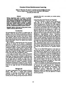
We consider two simple games: Nim-3: A simplified variant of the game Nim, where N tokens are on the table, each player can take 1, 2, or 3 tokens and the winner is the one who takes the last token. The state space has 2N states. The optimal strategy is to leave 3 + 1 tokens for the opponent. Although almost trivial, we are interested in situations where RL fails to learn the task or is considerably slow in learning it. TicTacToe: The board contains 3 × 3 fields, each player in each move marks (with X or O) a field and the winner is who gets “3 in a row” (horizontal, vertical, diagonal). The state space contains 5478 states. This is small enough that a standard minimax agent can perform exhaustive search for each state and find the best move. A state in strategic games is usually described by the current board position and the player who made the last move (so-called after state [3]). An example for TicTacToe is shown in Fig. 1. Following the ideas of Tesauro [2], the RL agent learns the game function V (st ), which ideally gives for each after state the probability that player p = +1, i.e., “X” will win. Given a certain board position, the strategy for player p = +1 is to select the next move which maximizes V (st+1 ), while player p=-1 (“O”) tries to minimize V (st+1 ). A state can be encoded by collecting row-by-row the board positions into a state vector with +1 for each “X”, “O” for each unoccupied field and −1 for each “O”. Together with the player who made the last move we get for example in Fig. 1 the following
Fig. 1. Some after states for the game TicTacToe
state representation for state s4 , which is a safe win for player “X”: s4 = {00 − 1, 011, −100, −1},
V (s4 ) = 1.000
(1)
Even for moderate games the state space is usually too large to be represented as a table and it is impossible to visit every state sufficiently often during learning. To overcome this problem, a function approximation scheme is used where each state s is transformed into a feature state g(s) and the function f (w; g(s)) with internal parameter vector w (the weight vector) approximates V (s). The TD algorithm aims at learning the function f (w; g(s)). It does so by setting up an (initially inexperienced) RL agent who plays a sequence of games against himself. It learns from the environment which gives a reward r ∈ {0.0, 0.5, 1.0} for { O-win, tie, X-win } at the end of each game. The main ingredient is the temporal difference (TD) error signal δt = rt+1 + γV (st+1 ) − V (st ),
(2)
where rt+1 is the reward for state st+1 (0 in a rewardless state, the game reward r when t + 1 is the final state) and V (st+1 ) is the game value for st+1 . The idea is to remember from state st the value V (st ) and the gradient ∇w f (w; g(st )) of the function f with respect to the weights w, to wait for the next state st+1 , and to apply then a learn step for the former state st . Thus the error signal aims at bringing the game value V (st ) closer to the (best) successor game value γV (st+1 ) in a rewardless state or closer to the sum rt+1 + γV (st+1 ) in a final state. The discount parameter γ is usually close to 1. Typical approximation functions are – a linear function f (w; g(s)) = w·g(s) (or the sigmoid of this linear function) – a backpropagation net with weights w and input g(s). In both cases the learning step uses a variant of gradient descent with the socalled eligibility vectors et . The core of the TD(λ)-algorithm is given as pseudo code as Algorithm 1. After the network is initialised with random weights, Algorithm 1 is called for G games to produce a trained RL agent. Usually the learning parameter α and the exploration parameter � are slowly decreased in the sequence of the games, e.g., α decreases exponentially from αinit to αfinal . For each of the games Nim-3 and TicTacToe we explore different feature sets which are defined in Tab. 1. As an illustration consider TicTacToe state s4 in Fig. 1, which gives rise to the following feature vectors in the sets T 1 and T 3, resp.: T 1 : g(s4 ) = (3, 0, 0, 2, 1, 0) T 3 : g(s4 ) = (3, 0, 2, 1, 3, 2, 0, 0, 1, 0, 0, 0, −1, 0, 1, 1, −1, 0, 0) Note that there is only a small difference between F zero and F 2 (the 1 is replaced by p), but this has a large impact on learning, as we will see below.
Algorithm 1 “Self-play”: Incremental TD(λ)-algorithm for strategic games Input: player p0 [=+1 (“X”) or -1 (“O”)] for the first move, initial state s0 , and a (partially trained) function f (w; g(st )) to calculate the game function V (st ). 1: Vold := f (w; g(s0 )) and t := 0 . with player −p0 in after state s0 2: e0 := ∇w f (w; g(s0 )) 3: for (p := p0 ; 1; −p → p, t + +) do . switch forever between players 4: select random number r ∈ [0, 1] 5: if r < � then select randomly an after state st+1 . explorative move 6: else select after state st+1 which maximizes p · f (w; st+1 ) . greedy move 7: get response V (st+1 ) := f (w; g(st+1 )) and reward rt+1 := r(st+1 ) from environment 8: calculate error signal δt := rt+1 + γV (st+1 ) − Vold 9: if st+1 is greedy move or st+1 is final state then 10: make learn step w := w + αδt et 11: end if 12: if st+1 is final state then break . exit for-loop 13: Vold := yt+1 := f (w; g(st+1 )) . because w has changed! 14: et+1 := γλet + ∇w f (w; g(st+1 )) . becomes et for the next iteration 15: end for
Table 1. Feature sets for Nim-3 and TicTacToe. Each feature vector is an M dimensional vector: (f0 , . . . , fM −1 ) for Nim-3 and (t0 , . . . , tM −1 ) for TicTacToe. Singlets in TicTacToe are lines (horizontal, diagonal, vertical) with exactly one token of player p, the rest of the fields being empty; similar for doublets and triplets. A crosspoint is an empty field belonging to at least two singlets of the same player. It characterizes an opportunity for that player. “Diversity” counts the number of different singlet directions for each player. Name F0 F1 F2 T1 T2
T3
Description Feature sets for Nim-3 fi = 1, if i tokens left; fN = player p (i = 0, . . . , N − 1) fi = 1, if i tokens left; fi+N = p, if i tokens left (i = 0, . . . , N −1) fi = p, if i tokens left; fN = player p (i = 0, . . . , N − 1) Feature sets for TicTacToe t0,1,2 : number of singlets, doublets, triplets for p = −1; t4,5,6 : number of singlets, doublets, triplets for p = +1; t0,1 : number of singlets, doublets for p = −1; t2,3 : number of singlets, doublets for p = +1; t4,5 : diversity O/X if p = −1; t6,7 : diversity O/X if p = +1; t8,9 : crosspoint count O/X; same as T 2 plus nine features containing the raw board position
dim M N +1 2N N +1 6 10
19
3
Evaluation
We measure the success of a trained RL agent by different metrics. Nim-3: The 2N possible outcomes of the game function V can be directly evaluated. If the value of p · V in a after state for player p with s = 4m tokens, m = 0, 1, 2, . . ., is larger than in the states with s+2, s+1, s−1, s−2, then the agent will play optimally on all possible moves and we term such an agent a success. TicTacToe: We evaluate in a set of 40 selected states whether the RL agent produces the same move as the optimal move suggested by the minimax agent (or produces an equivalent move having the same minimax score). The percentage of correct moves is a measure of success. This metric explores the state space if the 40 selected states cover relevant aspects of the state space. TicTacToe: In a tournament, the RL agent plays 500 games against other agents, either as player X (the starting player) or as player O. We measure the percentage of X-wins, ties, and O-wins. The success rate in a tournament is the simplest and, at the end of the day, most relevant metric. But, note that a tournament against the minimax agent will produce always the same moves and thus will explore only a tiny fraction of the state space. The success rate in the Nim-3 metric is measured as the average over 500 realisations of the RL agent. The results in Fig. 2 show the following: The earlier each curve rises to 1.0 the faster the RL agent has learned the concept. It is clearly seen that learning is faster without a sigmoid on the output and that the linear net learns considerably faster than its backpropagation companion. All runs use the feature set F 0, which is simpler to learn than F 1 or F 2. Of course the linear net can not learn each feature-output-relation. While the feature set F 1 is still linearly separable, the feature set F 2 is not. The linear net can learn F 1 as well, but not F 2. But, as Fig. 3 shows from the average over 500 realisations, also the backpropagation net has increasing difficulties in learning F 1 and F 2. It does not succeed at all in the case F 2, with sigmoid which is quite a surprising failure. Figure 4 shows the second measurement metric, the percentage of correct moves on selected states. It is quite easy to reach 50% or more, but difficult to achieve a figure above 85% on the average of 200 independent realisations. Single realisations can reach 100% correct moves. The learning curve in Fig. 4 shows quite surprisingly a decline in performance for feature set T 1 as G increases. As a general trend, the “richer” feature sets T 2 and T 3 show much better performance. The decline for G ≥ 104 in 3 of 4 learning curves is not yet fully understood. Finally we perform a TicTacToe tournament of 300 games between an RL agent, a minimax agent, and a random agent, where the latter chooses each move at random. The results shown in Tab. 2 are quite satisfactorily (no agent can do better than “tie” against the minimax agent). Although without any strategy, the random agent explores the full state space and it is not easy to win consistently against it. The percentages obtained here are about ten points
Fig. 2. This figure shows how fast different net types can learn Nim-3, as a function of the number of training games in self-play. The linear net without sigmoid in the output neuron learns ten times faster than the backprop net without sigmoid and 50 times faster than the backprop net with sigmoid. Parameters: αinit = 0.1, αfinal = 0.01, λ = 0 and γ = 0.9. The backpropagation net has six sigmoidal hidden neurons.
Fig. 3. Success rate in Nim-3 for different feature sets. Again nets without output sigmoid (solid lines) learn faster than those with (dashed lines). In all cases the net is a backpropagation net with six hidden neurons. The importance of correct feature-set selection is demonstrated: slow or no convergence on feature set F 2. 12 hidden neurons produce similar results. Other parameters are the same as in Fig. 2.
Fig. 4. Percentage of correct moves in TicTacToe for different feature sets. Each measurement point averages 200 independent realisations of a backpropagation net with 15 hidden neurons. Nets without output sigmoid (solid lines) learn faster in the initial phase, but nets with sigmoid (dashed lines) produce slightly better results as G increases. Best results are obtained with feature set T 3. Other parameters are the same as in Fig. 2.
higher (in the favor of RL) than the similar results reported in [4]. It has to be noted, that these results were achieved with a single (best) RL agent realisation, which is the same procedure as in [4].
4
Discussion
An important result is that a linear output neuron is advantageous in nearly all cases compared to an output neuron with sigmoid function. This holds both for the linear net and the backpropagation net. It is surprising at first glance, since a sigmoidal output in [0, 1] seems more appropriate for a function approximating V (s), the probability of a win for player X. The reason for slower learning convergence (or no learning success at all) might lie in the following fact: In the sigmoidal case the gradient ∇w f is a function proportional to f ·(1−f ) and thus becomes weaker as f approaches 0 or 1, the desired targets. Therefore “pulls” into the right direction have a smaller net effect than “pulls” into the wrong direction as they occur during the initial learning phase or while the correct concepts are not yet learned. Another interesting result is that the right selection of features is of great importance to the learning process, as Fig. 4 shows. Too few features or features
Table 2. Our results from a 300 games TicTacToe tournament. The RL agent is our backpropagation net with 15 hidden neurons, linear output function, trained on feature set T 3 over G = 10000 games of self-play. The minimax agent is a perfect player (recursive search of best move), while the random player chooses each move randomly. See Tab. 3 for comparable results by Stenmark [4]. X vs. O
X wins
tie
O wins
minimax vs. RL RL vs. minimax random vs. RL RL vs. random
0% 0% 0% 100%
100% 100% 18% 0%
0% 0% 82% 0%
not specific enough towards the learning goal might block the road to success. On the other hand too many features on top of specific features seldom do any harm, the RL agent quickly learns to ignore irrelevant features. Even if an additional feature is quite unspecific (as for example the field contents used as extra features in set T 3, which is on a single level not directly related to win or loss), it might help to make a formerly linearly inseparable task separable. This enables a linear function approximator to learn the desired behaviour quickly and robustly. This brings in front another topic which is well-expressed on Suttons RL FAQ page [5], but too often forgotten in RL applications in the literature: Sutton emphasizes the robustness and speed of linear nets and prefers them in first approaches to new RL-tasks as opposed to backpropagation or other non-linear function approximators. We feel in the same way and think that the results presented here might assure these statements. It pays off to think about features and their connection to the learning goal. The Nim-3 task and the seemingly similar feature sets F 0 and F 2 show that tiny modifications can be important: While F 0 contains the same information as F 2, it makes learning much easier. In the set F 2 conflicting concepts are overlapping and hinder the learning process. Note that in the set F 0 the input f4 = +1 always signals a win for player +1, while in the set F 2 the input f4 = 1 means a win if fN = +1, but a loss if fN = −1. The net has to learn
Table 3. Results as reported by Stenmark [4] on a TicTacToe tournament. The RL agent is a backpropagation net and was trained with 1 million games of self-play, yet it does not achieve the same performance as in Tab. 2. Entries in bold face highlight differences to Tab. 2. X vs. O
X wins
tie
O wins
minimax vs. RL RL vs. minimax random vs. RL RL vs. random
0% 0% 4.5% 90.5%
100% 100% 22% 9.5%
0% 0% 73.5% 0%
Table 4. Tournament results when playing TicTacToe against the agent ANN by Levkovich [7] which uses also RL and a feature set equivalent to our set T 1. RL(T 1) and RL(T 3) are our RL agents with feature sets T 1 and T 3, resp. Other parameters are the same as in Tab. 2. X vs. O
X wins
tie
O wins
ANN vs. RL(T 3) RL(T 3) vs. ANN ANN vs. RL(T 1) RL(T 1) vs. ANN RL(T 1) vs. RL(T 3)
7.4% 61% 24.1% 63.4% 16.2%
46% 18% 45.5% 16.3% 39.4%
46.6% 21% 30.4% 20.3% 44.4%
the “concept” (f4 · fN ), but the conflicting TD error signals hinder it to do so. A similar source of conflicts, namely the interference of redundant inputs was reported by Togelius et al. in their work on memetic climbers [6]. Finally we compare our results with other work: For the game TicTacToe many RL-implementations exist [4, 7]. The RL agent from [4] shows a 10% weaker performance on the random agent (Tab. 3), although it was trained 100 times longer (1 million games). But the difference is that their input was only the set of raw board positions. This demonstrates the importance of feature inputs. The RL agent in [7] is available as source code, so we ran several direct tournaments where both agents had the same number G = 10000 of training games (Tab. 4).1 The win rate of our RL agent with feature set T 3 was on average three or seven times higher than that of the RL agent ANN in [7], depending on whether our RL agent played as O or as X, resp. The performance of our RL agent with feature set T 1 was a bit weaker, still slightly above ANN. So RL(T 3) leaves the tournament as the best agent, even stronger than RL(T 1). As a general remark it is quite surprising that the different RL agents do not reach very often a tie or draw when playing against each other, as they do when playing against the perfect minimax agent or against themselves. The reason is probably that they did not encounter all variants of the other RL agent during self-play training, so both sides have their “vulnerabilities” when playing against each other. However, a better learning scheme seems theoretically possible where an agent learns a perfect strategy just from self-play. Yet it has not been achieved in an RL scheme with function approximation (where a learning step for state A can also influence the results for state B).
5
Conclusion and Future Work
Some insight has been gained in the way to configure RL learning agents. It has been studied in the case of strategic games but might as well be applicable to other control or learning problems with delayed rewards. A somewhat surprising result is that a sigmoidal output function is disadvantegeous in some tasks. 1
The source code of our implementation can be requested from the authors as well.
Another interesting failure is the decline of the RL agent to learn the Nim-3 task from feature set F 2, while rapidly converging on the very similar feature set F 1. This shows the importance of the right feature selection. Compared to other RL solutions on the TicTacToe task we find good results within only 1/100 of the learning steps reported in [4]. We plan to apply the results obtained here to more complex learning tasks, e.g., to the game Connect4 (state space complexity 1014 ). A number of parameters and algorithmic choices have to be tuned carefully, which we plan to do in a systematic way with Sequential Parameter Optimization (SPO), a recent and leading technology in statistical analysis [8]. The most interesting “parameter” seems to be the design of a sufficiently rich and goal specific feature set for a learning task. It seems interesting to develop automatic or semi-automatic procedures for feature selection and test their validity on different RL learning tasks. Guidelines for the design of feature spaces could be the following properties: – Is the feature distinctive with respect to the optimization goal, i.e., does at least one of the feature values reliably signal a win / a loss? – Can we generate complex features as combinations of primitive features which have increased distinctiveness? – Does a certain feature vector see too much spread in desired target values during learning? If so, probably different concepts of the learning task are mapped to the same feature vector and it might help to enrich the feature set to make these concepts separable. It is desirable to find meta strategies for the selection of the best feature sets independent from the learning tasks. We plan to use again SPO [8] for this task. The final goal is to develop RL agents which learn optimal behaviour from the interaction with the environment in a way more robust and faster than the current RL agents.
References 1. Sutton, R.S.: Learning to predict by the method of temporal differences. Machine Learning 3 (1988) 9–44 2. Tesauro, G.: TD-gammon, a self-teaching backgammon program, achieves masterlevel play. Neural Computation 6 (1994) 215–219 3. Sutton, R.S., Barto, A.G.: Reinforcement Learning: An Introduction. MIT Press, Cambridge, MA (1998) 4. Stenmark, M.: Synthesizing board evaluation functions for connect4 using machine learning techniques. Master’s thesis, Østfold University College, Norway (2005) 5. Sutton, R.S.: Reinforcement learning FAQ. http://www.cs.ualberta.ca/ sutton/RLFAQ.html (2008) Cited 20.4.2008. 6. Togelius, J., Gomez, F., Schmidhuber, J.: Learning what to ignore: Memetic climbing in weight and topology space. To appear in Congress on Evolutionary Computation (2008) 7. Levkovich, C.: Temporal difference learning project. www.geocities.com/ chen levkovich/tdlearningproject.html (2008) Cited 10.3.2008. 8. Bartz-Beielstein, T.: Experimental Research in Evolutionary Computation—The New Experimentalism. Natural Computing Series. Springer, Berlin, Heidelberg, New York (2006)