Relation-based Message Routing in Wireless Sensor ...

Relation-based Message Routing in Wireless Sensor Networks

127

7 0 Relation-based Message Routing in Wireless Sensor Networks Jan Nikodem, Maciej Nikodem, Marek Woda and Ryszard Klempous Wroclaw University of Technology Poland

Zenon Chaczko

University of Technology Sydney Australia

1. Introduction Sensor networks and their related topics represent some of the greatest and challenging possibilities in the research field that have come about in recent years. Emerging technologies like wireless sensor network (WSN), standards enabled legacy sensors, ubiquitous and cloud computing, middleware, communication systems, internet protocols (IP) and next generation networks are leading to a set of new paradigms where wireless sensors can be treated as vital components of common infrastructure and a shared resource with an ability to serve multiple and concurrently executing applications run by various users in distributed environment. This is in strong contrast to traditional concepts where dedicated sensor devices are being physically and logically hard-wired to communication and computing infrastructure serving very specific and dedicated data/information processing applications. Wireless sensor networks consist of a number of small electronic devices (nodes) distributed in an area that by far exceeds the communication range of a single sensor. Message routing is one of the most important issues in such networks. This is mainly due to the large number of nodes, variety of possible communication paths, restricted power source and variability (in time and space) of environmental conditions in which the WSN operates. A shared communication channel and restricted communication ranges require that nodes of the WSN cooperate and/or coordinate their actions while messages are routed from nodes to the base station (BS). It is a well-known idea Descartes & Lafleur (1960) to solve large and complex problems by dividing them into smaller and possibly simpler tasks. The most crucial element of such an attempt is to decide how to divide the problem in order to get a problem that can be solved efficiently and, what is more important, can be used to find a solution to the original problem. A distributed system, such as a WSN, is traditionally seen as a set of spatially distributed nodes that communicate, coordinate their actions and inform other nodes about their status using special messages sent over the communication channel Dollimore et al. (2005). Such a system is usually assumed to be isolated from the outside word – even if it measures its parameters and/or listens to the status messages from other nodes, it is still not affected by the environmental conditions and its changes. We are going to look at such a system as it

128

Smart Wireless Sensor Networks

consists of independent elements that adjust their actions according to the actual situation in their neighbourhood and WSN in order to achieve globally defined goals. Surroundings of each node is composed of two elements: • neighbourhood – a set of WSN elements (i.e. nodes) that are in the surroundings of the node, • environment – a set of elements that are in the surroundings of a node, influence its behaviour, but are not elements of the WSN. The above approach enables to describe any system as an open system in which communication activity adapts to stimulus that originates both from system elements as well as from environment. This enables the system to respond to harsh and unpredictable situations that may be beneficial in many applications. When analysing WSN it is important to capture four related components: • independence of WSN elements, • cooperation, and • communication between WSN elements, • interaction of elements with the environment. This chapter focuses on communication in a distributed system such as a WSN. The main purpose of communication in WSNs is to retransmit messages and route them to the base station. Our interest in distributed WSNs is not only due to spatial distribution of nodes of the network, but also due to the fact that decisions on message routing and communication paths are taken in distributed manner as an effect of cooperation between nodes.

2. The relational model of communication in WSN Investigation of activities in wireless sensor network can be based on relational model of cooperation between nodes of the network Nikodem (2009). Relational model captures dependencies (relations) between nodes of the network and defines actions that nodes may take in different situations. Actions are taken by every node individually, so the relational model can be used to describe independent elements that cooperate within the network in order to achieve globally defined goals. since the relational model reflects the nature of real WSNs, therefore, it includes all previous proposals to efficient network organisation, communication and routing. Moreover, it enables to construct new algorithms that will achieve globally defined goals through local actions taken be each node of the network. 2.1 Actions and relations between nodes

Communication activity in WSN can be described using three binary relations defined over set of actions - Act. Set of actions contain all activities that can be carried out by every node of the network individually but with respect to other nodes and environment (i.e. situation in the neighbourhood). Ability to execute specific action depends on the state of the node (e.g. network establishment actions, network management, and normal operation) and its execution cause the state of the node to be changed. Therefore, all actions that can be taken by nodes of the WSN are defined over a Cartesian product of set of nodes Nodes and set of all possible states States: Act : Nodes × States → States. (1)

Relation-based Message Routing in Wireless Sensor Networks

129

Measurement of environment parameters, data aggregation, sending messages to a single (or group) node and message receiving are examples of actions that can be taken by nodes. Since nodes are autonomous, therefore each node can execute actions independently from other nodes. Undoubtedly, this is an advantage since this enables nodes in a different part of the WSN to perform various (possible related) actions simultaneously. On the other hand a number of actions become essential only when two or more nodes cooperate. In such situation cooperation requires that nodes execute actions that are related which is formally denoted as: (1)

(2)

ai R a j , (1)

(2)

where ai , a j

(k)

∈ Act and ai (1) ai

(2)

denotes i-th action that is executed by k-th node. Eq. (2) should (2)

is in relation with a j . Relations are used to determine actions that are be read as: action related to each other and are either executed together (but not necessarily in the same time instant) or cannot be executed together. Since nodes can execute a vast number of actions that can be part of different relations, therefore relations have their names and symbols. Since this chapter focuses on communication, therefore, we will only consider communication related relations and simplify the notation. From now on sending and receiving a message will be denoted as x where x is an ID of node that is either sending or receiving the packet. Whether node x sends or receives the message will arise from the context or will be explained in the text. To describe a variety of possible dependencies between different elements of real world WSN it is enough to define three elementary relations Jaron (1978); Nikodem (2008): • subordination - π, • tolerance - ϑ, • collision - κ. When message sending and receiving actions are considered then subordination xR πyS ,

(3)

means that node y receives data whenever node y send it. Subordination is transitive which means that if x is subordinated to y and z is subordinated to x then z is also subordinated to y: xR πyS and zR πxS ⇒ zR πyS .

(4)

Subordination is antisymmetric which means that if x is subordinated to y then y is not subordinated to x: xR πyS ⇒ ¬ (yR πxS ) . (5)

We can define a set Π of pairs of nodes of the WSN that are in subordination relation. This set consist of ordered pairs of nodes such that: Π = { x, y | xR , yS ∈ Act and xR πyS }

(6)

When dealing with communication tolerance relation between nodes x and y xR ϑyS

(7)

means that x may receive messages send by node y. When x tolerates y then it is less likely that node y sends messages to x - y prefers subordinated nodes. Nevertheless, y may send message

130

Smart Wireless Sensor Networks

to x and whenever this happens node x will receive the message and route it towards the base station. In contrast to previous relation tolerance is symmetrical xR ϑyS ⇒ yR ϑxS ,

(8)

but is not transitive. Subordination and tolerance relation can be composed - if x is subordinated to y and z tolerates x then z also tolerates y: xR πyS and zR ϑxS ⇒ zR πyS .

(9)

Set of all nodes that tolerate each other is a set of pairs < x, y > such that Θ = { x, y | xR , yS ∈ Act and xR ϑyS } .

(10)

It follows From the definition of relations π, ϑ for corresponding sets of subordinated and tolerated nodes (Π and Θ) that Π ⊆ Θ. (11) The final relation that we need to consider is the relation of collision which for data transmission and reception activities in WSN specifies all those sensor nodes that don’t exchange messages among themselves. The relation of collision between node x and node y is denoted as: xR κyS , (12)

The above relation takes place when a node x does not receive any messages transmitted by the node y, including both broadcasted and explicitly addressed messages from the node y to the node x. Additionally, if a node x has a collision relation with node y and the node z is subordinated to the node x, then the node z has also a collision relation with the node y. This can be expressed as: xR κyS ∧ zR π xS ⇒ zR κyS . (13) The relations of tolerance and collision are mutually exclusive therefore only those WSN nodes that are not in a relation of tolerance can remain to stay in a relation of collision. Hence, if we denote a set of nodes that remains in relation of collision as: K = {< x, y >| xR , yS ∈ Act ∧ xR κyS },

(14)

then the sets of nodes that remain in relations of tolerance and collision meet the following criterion: Θ ∩ K = ∅. (15)

Since, Π ⊆ Θ also applies therefore sensor nodes that are both in relation of tolerance and subordination cannot remain in relation of collision Π ∩ K = ∅. 2.2 Neighbourhood, Neighbouring and Environment

(16)

When studying multi-hop communication in sensor networks it is not possible to omit such specific aspects of WSN as sensor node cooperation. Due to limited radio range, the majority of nodes in the WSN are not able to transmit data directly to the base station, therefore the nodes have to rely on the mechanism of retransmission offered by other nodes in their surroundings. Wireless sensor networks are truly distributed systems where sensor nodes characterised by limited communication resources cooperating among each other in order to

Relation-based Message Routing in Wireless Sensor Networks

131

support the network infrastructure activity as a whole. Events and entities that are in the perception range of a node belong to its surroundings. In the set that we call the surroundings we can identify two distinctive subsets: neighbourhood and environment. Considering that we are interested in communication aspects of WSN, the concept of neighbourhood is particularly significant; hence we dedicate this concept in our further investigation. In WSN related literature the definition of neighbourhood is frequently used, often becoming a basis for the definition of several routing algorithms Braginsky & Estrin (2002); Burmester et al. (2007); Manjeshwar & Agrawal (2001); Younis & Fahmy (2004). Let us begin from explaining the meaning of Map(X, Y) expression that can be defined as a collection of mappings of set X onto set Y (surjection). Let us define Sub(X) as a family of subsets X and the neighbourhood as N ∈ Map( Nodes, Sub( Nodes)). (17)

Furthermore, if N( x ) belongs to neighbourhood of the node x and N(S) is a neighbourhood of the set S of nodes then, using the neighbourhood relation (here denoted as η) we can define a collection of nodes which are neighbours of the given node x as: N( x ) = {y | y ∈ Nodes ∧ xηy},

(18)

and denote the set of neighbours of all nodes that belong to the set S as: N(S) = {y | y ∈ Nodes ∧ (∃ x ∈ S | xηy)}.

(19)

In this discussion, we assume that the neighbourhood relation is a symmetric: x η y ⇒ y η x.

(20)

This implies, that if a node x remains in a neighbourhood relation with y (i.e. x is able to communicate with y) then the node y is also in a neighbourhood relation with x. In WSN literature several various locality models were proposed Nikodem et al. (2009). Various benefits and drawbacks of sensor node clasterization or unique transmission paths in context of the applied definition of neighbourhood are also discussed. However, the most accepted approach for defining the locality is the one based on the concept of the neighbourhood that is derived from the technological limitation of radio communication. In some specific situations the partitioning of network into clusters can be very beneficial, to a degree this can be seen as an oversimplification that makes our computation much easier. However, the trade-off is a reduction of the solution space. In the case of a singular retransmission path the solution space consists only of one element. Let us consider the neighbourhood family of N = {Ni | i ∈ I} for which the following conditions are met: (∀i ∈ I | Ni = ∅)(∪i Ni = Nodes), (21)

(∃ i, y ∈ I | i = j)(Ni ∩ N j = ∅).

(22)

(∀y ∈ Nodes)(∃ i ∈ I | y ∈ ∩Ni = ∅).

(23)

This translates onto a local mode (for each node) and takes the form of:

The expression ∃ can be translated as: "there are as many instances as the structure of the network allows for". The neighbourhood obtained when taking this approach can be interpreted as the most natural of all possible instances that can also guarantee the maximum retransmission capabilities for all allowable solutions.

132

Smart Wireless Sensor Networks

Referring back to concepts of surroundings (S), neighbourhood (N) and environment we could observe that:

((N ⊂ WSN ) ∧ (E  WSN )) ∧ ((N ∪ E ⊂ S) ∧ (N ∩ E = ∅)).

(24)

Neighbourhood is a collection of all of the neighbouring surrounding that belong to the WSN, while the environment (E) consists of all of the elements of surrounding that do not belong to the wireless sensor network but that do have an effect on its behaviour. 2.3 Forming Actions - Chains

Relational dependencies of the chain functions of WSN in most cases describe connections between the neighbouring nodes and adapt general principles of neighbourhood. To deal with it, let us focus on the relation of subordination π. Out of all four relations only this one is transitive, which allows us to model the retransmission paths. The π relation which is both transitive and reflective, forms a preorder in the set of actions Act (1). Further investigation requires a stronger order of the set of actions Act. Introducing a partial order does not appear difficult. In real time applications, nodes are distributed more or less randomly over a given area (i.e. they may be dispersed out of a aeroplane). In the case where two network, nodes are found very close to each other, one of them becomes tacit (mute) and in reserve. In this way, a singular communication node substantially greater robustness and survivability is formed. In mathematical terms, such “binding” of two elements can be expressed as:

(∀ x, y ∈ Act)( x π y ∧ y π x ) ⇒ (y = x ).

(25)

The above expression shows that subordination happens asymmetrically which in turn may lead to a partial set order (asymmetric preorder). Therefore, the set of actions Act is partially ordered (poset). In the discussed formal apparatus we have a stronger relationship than the one indicated in expression (25). As shown in (5), the subordination relation is of an antisymmetric nature; hence this is equivalent to irreflexivity as every relation that is antisymmetric is both asymmetric and irreflexive. Indeed in WSN, a situation when a sensor node transmits to itself does not belong to a category of logical behaviours. Irreflexivity put together with transitivity provides a strict partial order. The set of actions Act being finite and partially ordered can be represented in many ways as any two argument relation can be represented in a form of a directed graph or a diagram. For such a graphic representation we can use the Hasse diagrams which can help us to show the subordination relation between pairs of elements and the whole structure of partial classification of the set of actions. Although, the Hasse diagrams are simple and very intuitive tools for dealing with finite posets, it turns out to be a difficult task to draw ”clear” diagrams for more complex situations when we try to represent all possible communication links in the structure of WSN. In most cases when we apply the Hasse technique by first drawing a graph with the minimal elements of an order and then incrementally adding other missing elements we may end-up producing rather poor and unreadable diagrams where internal structure and symmetries of the order are no longer present due to a large number of connections. Therefore, we need to search for a better solution. Our approach using the relations may in the future lead to more viable solution for the representation of connectivity in WSN. In multi-hop sensor networks, the subordination relation that reflects communication aspects of WSN, is not a relation that is cohesive or finite. This means that:

(∃ x, y ∈ Act)(¬( x π y ∨ y π x )),

(26)

Relation-based Message Routing in Wireless Sensor Networks

133

hence, there are elements for which such a relation does not take place, thus the subordination relation can be described as a set of a partial order (poset). It is possible to select subsets of such a set that are linearly ordered so that the partial order will additionally meet the condition of cohesion such as: (∀ x, y ∈ Act)( x π y ∨ y π x ). (27) It needs to be noted that this expression contradicts the previous one. In multiplicity and partial order theories, ordered subsets for which the order relation is found to be cohesive are called chains. To form the chain we shall define the subordination relation setting by the following induction: π n = π n−1 ◦ π, . . . π 2 = π 1 ◦ π, π 1 = π. (28)

Hence

π n = {< x, y >|< x, y >∈ Actn−1 × Act},

(29)

Ascπ (y) = {z ∈ Act | (∃n ∈ N)(yπ n z)},

(30)

Desπ (y) = {z ∈ Act | (∃n ∈ N)(zπ n y)}.

(31)

where x shall be called the direct successor of y, while y will be called direct predecessor of x. Forming the communication activities in multi-hop WSNs is the fundamental problem because there is a question whether messages from the network area can be passed onto the base station. On a global scale (this involves the whole WSN), to build suitable structure that allows us to find the answer for this question we could draw on a concept from the theory of multiplicity - transitive closure of 2-argument relation of subordination π on the set Act. However, in this work, the problem of solving the communication activity is perceived from the local level (node neighbourhood). Therefore, we shall consider a case when a packet is transmitted from the node y and after certain number of retransmissions should reach the base station (BS). Applying the setting of subordination relation π, for each sensor node y we define sets of its ascenders Asc and descenders Des using the following expressions:

Expressions (30),(31) define sets with full communication space of the node y. One of our main aims, however, is to find an answer to the question “to whom send a packet in open space?” hence we need to pay more attention to the set Desπ . It is worth to notice, that for a packet to arrive from the sensor node y to its destination at the node BS it is necessary for the base station to be one of the elements of the set Desπ . Additionally, we could form many subsets of the Desπ set and some of these subsets may help us to determine communication activity in WSN. Among the subsets of Desπ , we can distinguish two types of subsets: • four sets that are partially ordered, and • family of well-ordered chains (linearly ordered sets) The selected ordered chains can be defined as: Desmin π ( y ) = { x ∈ Desπ ( y ) | BS π x )}.

(32)

The subset (32) contains the selected nodes that are the direct ascenders of the base station (BS). Hence, only the retransmission that involves these nodes allows the packets sent from the node y reaching the BS. The power of this set determines the maximum number of packets that can be delivered from the node y to the BS. Second subset Desmax π ( y ) = { x ∈ Desπ ( y ) | x π y )},

(33)

134

Smart Wireless Sensor Networks

contains the nodes that are direct followers of the y node, in other words, these are the nodes that are required to execute the retransmission of the packet issued from the node y. The power of this set determines the maximum number of packets that could be sent from the node y to the BS. Third subset n Desmis π ( y ) = { x ∈ Desπ ( y ) | ¬(∃ n ∈ N)(BSπ x )},

(34)

contains nodes that become the dead end on the paths to the base station. A packet that arrives at such a node does not have even a chance to reach the BS. The last subset p f ex

Desπ

(y) = { x ∈ Desπ (y) | Card(Ascπ ( x )) > 1},

(35)

is made up of nodes called pontifixes that are located at intersections of the packet routes. These nodes become the bottlenecks on the routing path from node y to the BS. Skilful shaping of the communication activity allows for the best utilisation of these elements. The power of the set of pontifixes defines the capability of packet to escape from one routing path onto another during the retransmission to the base station (BS). From the perspective of shaping the communication activity in WSN, the second most interesting subset group Desπ (y) represents a family of chains Chnπ (y) that constitutes linearly ordered subsets. For each iteration of the Chniπ (y) chain the following condition applies:

(∀Chniπ (y) ⊂ Desπ (y) | i ∈ I)(BS = ⊥ ∧ y = ),

(36)

where the symbol ⊥ denotes the smallest element BS and the symbol  denotes the biggest element (y).

3. Communication towards base station In a wireless sensor network nodes are responsible for the collection of information (individual action) and forwarding them to the base station (collective action). As it was described previously, such action may be described using the three relations - subordination, tolerance and collision. Subordination relation is particularly important, because of its transitivity and asymmetry, and it was used in the developed simulator. At first, let’s consider subordination relation only and suppose that the node x is a source of information. Then, the set Π( x ) contains all nodes, to which x can send messages directly. Using the subordination relation, a node that receives the information is able to forward it to its neighbors that are in the subordination relation with it. Therefore, we can define the set of the node descendants that contains all nodes to which the message may be sent to: Desπ ( x ) = {y | (∃n ∈ N)(yπ n x )} ,

(37)

where yπ n x indicates that there are n intermediate nodes y(i) such that one can build a chain of relationships yπyn , yn πyn−1 , yn−1 πyn−2 , . . . , y2 πy1 , y1 πx. (38)

When subordination reflects direction towards the base station then it is ensured that the base station belongs to the set Desπ ( x ) for each node x. Therefore, each message generated by x will eventually reach the base station. Moreover, it follows from the properties of subordination relation and the fact BS belongs to Desπ ( x ) that a message sent from the node x and retransmitted to subordinated nodes, always reaches the BS (assuming that all nodes on the

Relation-based Message Routing in Wireless Sensor Networks

135

communication path have enough energy). This is due to transitivity property of the subordination relation and the fact that in chain of relationships (38) we have yi πx for every i = 1, 2, . . . , n and yi πy j for any i > j. Since the subordination relation is asymmetric, so in the chain of relationships each node occurs only once - otherwise, if y i +1 = y j

(39)

for some i > j then from the fact that yi+1 πyi follows that y j πyi . However, since i > j therefore yi πy j and so the relation becomes symmetric which contradicts the assumption (5). This means that in sequence (38) each node can occur only once. Therefore, and due to the fact that Desπ ( x ) is finite and contains the BS follows that for every x there exists a finite subordination relationship chain that leads to the BS, i.e.: BSπyn , yn πyn−1 , yn−1 πyn−2 , . . . , y1 πx.

(40)

The above property results directly from the definition of set Desπ ( x ) that includes only these nodes that are closer to the BS than node x. As a consequence each node yi in relationship chain (40) is closer to the BS then x and y j for any i > j. If x is located in the communication range of the BS then set Desπ ( x ) is a singleton that consists only of the BS. Set Desπ ( x ) consists of a number of nodes y that are subordinated to x and, in connected networks (i.e. networks in which each node can communicate directly or using retransmission with BS), constitute one or more relationship chains. These chains may differ in number of elements but always lead to the BS. Similar properties do not hold for tolerance relation since BS does not necessarily belong to Desϑ ( x ) = {y min(∃n ∈ N)(yϑn x )} .

(41)

Moreover, there is no guarantee that yi = y j in the tolerance relationship chain yϑyn , yn ϑyn−1 , . . . , y2 ϑv1 , y1 ϑx

(42)

for any combination of i = j. This is a direct consequence of symmetry property that may lead to loops in chain where part of the chain begins and ends with the same node, e.g. xϑyn , yn ϑyn−1 , . . . , y2 ϑy1 , y1 ϑx.

(43)

As a result tolerance relationship chain may be infinite even if Desϑ ( x ) is always finite (since number of nodes in the network is finite). Above considerations present that tolerance relation itself is not sufficient to guarantee that cooperation within the sensor network will lead to proper routing of messages (i.e. that messages will reach the base station). However, tolerance has features that make it very useful as an auxiliary to the subordination. In real life application of WSN it may be particularly useful to cope with locality effects - this corresponds to situations when divided problems cannot be solved or does not improve the overall result. Similarly in WSN, tolerance will enable routing paths variation in order to prevent message loss (e.g. due to dead ends). In an extreme case tolerance relation (that is symmetric) may force a node to send a packet back to its ascender in order to find an alternative routing path. The combination of subordination and tolerance relations allows drawing on advantages of both relations. Subordination ensures that messages always reach the base station while tolerance increases by far the number of available communication paths.

136

Smart Wireless Sensor Networks

Main components of simulator

Information window files Sim2010About.m Sim2010 About.fig

Sim2010.m / Sim2010 .fig

Simulation supporting components

Simulator configuration

Sim2010Config.m Sim2010.fig

*.m

Fig. 1. Simulator architecture - key components

4. Simulation of WSN communication behaviour In order to present the relational approach that can model behaviour and operation of WSN we have developed a network simulator. Our simulator models behaviour of every single sensor that operates independently in order to meet globally defined criteria and with respect to situation in its environment. 4.1 Simulator

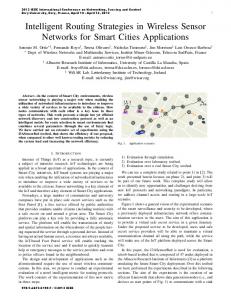
The MATLAB environment is required for set up and proper operation of the simulator. The simulator was written and had been tested in MATLAB version R2009b. Only the basic features of the MATLAB environment were used, so no additional tool kits (Toolboxes) are required. The architecture of the simulator is presented in Fig. 1. The entry point of the simulator is Sim2010.fig file which starts the simulator GUI. Work with the simulator Fig. 2 starts from parameters being setup (Phase I). This includes such parameters as network size, number of sensors, etc. This stage is surmounted by the deployment of sensors in the defined working area, visible in the visualisation area of the main simulator. The first action undertaken in Phase II, is the selection of one of the seven algorithms available in the simulator. Then, depending on the choice made, one can change the default parameters of the algorithm. At this stage, one can also decide how to present the results of simulation and its detail by setting additional parameters in the configuration window. Approval of the configuration changes made in this step allows for the transition to Phase III. Simulation begins when the RUN SIM button is pressed. From that moment, the simulation runs, with time as well as simulation results/parameters being visualised on the screen in the form of graphs and numerical results. Simulation can be also saved to an AVI file. During the simulation, a user can control it (stop and resume it), using the simulation control panel or configuration window to change the appearance of visualisation window. Completion of the simulation process ends PHASE III. Pressing the RESET DATA button, allows the user to jump back to the first stage and resuming simulation from the beginning (possibly with new parameters). Fig. 3 shows the main window of the simulator in which the basic parameters of WSN are defined, the simulation is visualised and information about the current state of the simulation (number of loops, number of messages etc.) and values of network parameters

Relation-based Message Routing in Wireless Sensor Networks

137

Phase I: Sensors placement Network dimension

Energy parametrs

BS location

Number of Sensors

Sensors distribution

Phase II: Algorithm selection – simulation parameters set up HEED

Authors Algorithms

Simulation parameters

Visualization parameters

Algorithms parameters

Simulation steering

Save results

Phase III: Simulation Change view

Network visualization

Parameters visualization

Fig. 2. Main simulation phases (the average cost of energy, lifespan, etc.) are presented. The basic network parameters that can be entered by the user are: • size of the network and its area - it is determined by defining a rectangular area in which WSN nodes will be deployed. Because one of the vertices of the area is permanently located at the point (0,0) this area is defined by specifying the length of two sides of the rectangle along the X and Y axis ("Network Size" field). It should be noted that currently the simulator operates for a two-dimensional network, which means that it is not possible to determine the size of the nets along the Z axis. • position of the base station - we have assumed that there is only one base station in the simulated WSN that can be located at any point of the network area. It is common to place the base station in a corner of the area which is the worst possible position • number of parameters and sensors - simulator allows to control such network parameters as the number of WSN nodes deployed ("Sensor - Number"), the maximal communication range of a single node ("Sensor - Range") and initial energy of each node ("Sensor - Energy"). In determining the number of nodes and their maximum range, one has to remember that these parameters are related to the size of the network. Setting too few nodes, or too short communication range can cause the network to be disconnected (some nodes of the network will not be able to communicate with the base station). Given network area ( P) and the maximum communication range of a node ( Rt ), the number of nodes required to ensure network is connected, can be estimated. Note that if in each circular area of the diameter Rt /2 at least one node is located then any two nodes located in two adjacent areas will be always able to communicate directly. This will be ensured regardless of their position within this area. Since the entire network area is rectangular, we assume that the area of Rt /2 diameter can be approximated by a

138

Smart Wireless Sensor Networks

Fig. 3. Main simulator window square of diagonal Rt /2, inscribed in the circle. If so then the number of areas that will fit on the entire network is equal to R2 N = √t . 2 2P

(44)

Once the number of areas is known, one can estimate the number of nodes to be scattered in the network that ensures each of N areas is covered with at least one node. This problem is equivalent to the ball-and-bins problem in which balls are thrown randomly to bins, which is the well-known in mathematics. It was presented that when   R2 R2 √t n = 2N log N = √ t log , (45) 2P 2 2P nodes (balls) are used then the probability that there is at least one node (ball) in each area (bin) is close 1.0. It should also be noted that this estimate is inflated due to the assumption that the area covered by communication range of a single node is square rather than circle. In addition to these parameters, the user can also influence the arrangement of nodes in the network. The simulator assumes that nodes are distributed evenly throughout the network (which is the assumption commonly adopted in the literature), however, one can control this distribution by identifying the seed used to generate sequences of random numbers. Using the drop-down list one can specify if the distribution of nodes should be completely random, or random with a seed that is entered by a user - in that case one must select "By Defined Seed" and enter the value of seed in the "Seed" window. Because of this, the same distribution

Relation-based Message Routing in Wireless Sensor Networks

139

of nodes in the network can be generated repeatedly, and thus one will be able to compare the actions on the same network with various parameters of the simulation and relations settings. The same window enables to determine which routing algorithm will be used for communication ("Type of algorithm" field). At this moment, the simulator implements three groups of algorithms in seven different variants. The groups are: • shift register, • energy balanced, • HEED, and differ in the idea of operation, criteria for selecting communication paths (consecutive retransmissions) and the principles of relations ordering. The main difference between the first two groups and HEED is that HEED is a standard hierarchical protocol Younis & Fahmy (2004), which does not use the relationship mechanism. The remaining two groups differ in rules that are used to order nodes within relations. For group of ’Shift register’ algorithms ordering takes place only once - after the deployment of nodes, during the initialisation of the network. This distinguishes these algorithms from ’Energy balanced’ where ordering takes place after every message sent by a node (sort is made by nodes that have sent, received or heard the message exchanged between neighbouring nodes). For both groups, the ordering concerns part of all WSN nodes. This is determined by setting a percentage of nodes in ’Sorted nodes [%]’ window. The value determines what portion of nodes will sort their neighbouring nodes according to their proximity to the growing distance from the base station (for groups ’Shift register’) or decreasing amount of remaining energy (for the group ’Energy balanced’). Remaining nodes do not sort their neighbouring nodes, which means that the order neighbours in the relation depends on the order in which node learnt of their existence. Relation for each node is represented in simulator as a vector (Register) of neighbouring nodes. Order of nodes within the vector corresponds to the relation ordering between nodes. Seven routing algorithms available in the current version of the simulator consist of: • Shift register - this is the algorithm in which each node neighbourhood (represented as a vector) behaves like a cyclic shift register, the shift occur only within a subordination relation, and messages are always sent to the first node from the register. The parameter of this algorithm is the intensity of the other subordination relation that determines the number of neighbours who are subordinated to the node. This parameter determines how many neighbours (counting from the beginning of the vector) are taken into consideration when node is about to send the message. • Shift register [%] - an algorithm is similar to the previous one but the intensity of the subordination relation is expressed by specifying the percentage of neighbours that are in a subordination relation rather than the number of nodes. • Shift register [Card(Π) = k] - in this algorithm the subordination relation includes only neighbouring nodes that are closer to the base station than the current node. Compared with the ’Shift register’ algorithm, the difference is that in ’Shift register’ subordination relation may consist of nodes that are more distant from the base station than the current node. In the current algorithm, this situation will never take place, although there is no certainty that the best neighbours (the closest to the base station) will be in a subordination relation. For example, this may happen if the registry (that represents the relation) is not sorted.

140

Smart Wireless Sensor Networks

Fig. 4. Parameter Sorted Nodes [%] in the configuration window • Energy balanced - this is an algorithm in which the subordination relation is composed of a number of neighbours in the left part of the vector (either sorted or not) and the number of nodes in relation is an algorithm parameter. The message is sent to the first node from the vector. After each messages sent, the node sorts this vector according to the amount of residual energy in neighbouring nodes - see description of sorting parameter ’Sorted nodes [%] earlier in this section. • Energy balanced [%] - this algorithm is similar to the previous one but the difference is that the intensity of the subordination relation is determined by indicating the percentage of the neighbouring nodes that are in the relation. • Energy balanced [Card(Π) = k] - similar to ’Shift register [Card(Π) = k]’ the algorithm also restricts the subordination relation to only these neighbours that are closer to the base station than the current node. • HEED - this is one of the most popular hierarchical algorithm, which defines how to group neighbouring nodes into clusters and transmit messages in the WSN. This algorithm has been implemented in order to compare with our proposal of relational based routing and communication. 4.2 Neighbourhood organisation and network communication efficiency

In the self-organisation phase executed prior to the proper operation of the network, each node collects information about its neighbourhood. Then, using the globally defined metric (expressed in number of retransmissions or the Euclidean distance from the Base Station), each node organises (i.e. sorts according to the residual energy in neighbouring nodes) its neighbours. Number of nodes in the network, which make such an arrangement, is determined by one of the parameters and defines the degree of the neighbourhood ordering. We have evaluated the impact of this parameter on the size of the communication area (that is area covered by nodes that take part in message routing), the number of intermediate nodes and energy efficiency of the algorithms used. The ’Sorted Nodes [%]’ parameter specifies the percentage of nodes that sort their neighbouring nodes according to their growing distance from the base station. Other nodes do not sort the neighbourhood, which means that the order of neighbours depends on the order in which the node "learnt" of their existence. In the rest of the chapter, results of simulations and conclusions are presented. All simulations were carried out with fixed values of parameters. These are presented in table 1. Changing the number of organised neighbourhoods has a significant impact on the efficiency of all tested algorithms. And so, when the parameter ’Sorted Nodes [%]’ had value 10% for both algorithms ’Shift register [Card(Π) = k]’ and ’Energy balanced [Card(Π) = k]’ then communication area is either very large Fig. 5 or large Fig. 6. It is worth noting that the algorithms from the group of ’Energy balanced’, when working with the same parameters, are characterised by a lower

Relation-based Message Routing in Wireless Sensor Networks

WSN parameters Number of sensors WSN area Position of the BS Sensor communication range Initial node energy Energy cost of message sent Simulation parameters Number of messages to send Communication to the BS Number of iterations Deployment of nodes Table 1. WSN and simulation parameters

141

300 100×100 x=1, y=1 20 300 5 300 from one selected node 300 random with fixed seed equal 10

average number of intermediate nodes required to route messages to the base station. When value of the parameter ’Sorted Nodes [%]’ changes from 10% to a maximum value of 100% then there is a diametrical improvement for both families of algorithms. Both paths have a less complicated shape - similar to the line, and thus lead to a base station with a smaller number of hops, which in turn results in improved energy efficiency. 4.3 Principles of retransmitters selection and area of the communication size and energy efficiency

Algorithms from the ’Shift register’ group can be divided due to the selection of successors (the following nodes in the routing path of a message that is transmitted to the base station): • numerical - the value of the parameter ’Reg. capacity’ defines the number of neighbouring nodes, from which the successive node is drawn when messages are about to be send, • percentage - similar to previous but the value of the parameter ’Reg. capacity’ defines the percentage of neighbours that will constitute the set from which the successive node will be drawn, • directional - the value of the parameter ’Reg. capacity’ defines the percentage of neighbours that constitute a set Desmax π ( x ) - set of nodes subordinated to the actual node (x). 4.3.1 Numeric vs. percentage selection

Numerical selection is the least effective method because it allows for the selection of retransmitters without any restrictions; even those nodes can be selected that are outside the desired direction toward the base station. This type of selection of retransmitters does not take into consideration the number of nodes in the neighbourhood that is a property of each node of the network, and may differ significantly throughout the network. Fig. 7 presents how selection of the number of potential retransmitters, appropriate to the number of nodes in the neighbourhood improves the communication efficiency. The ’Reg. capacity’= 10 allows sending the same number of packages, but without reaching the state of energy depletion in some nodes. For example, it follows from Fig. 7 that Card (Desmax π )=10 is the best value. However, this may not be true for the other nodes. Our tests show that it is the more favourable approach to use percentage selection, where Card (Desmax π ) corresponds to the number of nodes

142

Smart Wireless Sensor Networks

Fig. 5. Algorithm ’Shift register [Card(Π) = k]’ with ’Sorted Nodes [%]’ parameter equal 10% (left) and 100% (right) - retransmission path view

Fig. 6. Algorithm ’Energy balanced [Card(Π) = k]’ with ’Sorted Nodes [%]’ parameter equal 10% (left) and 100% (right) - retransmission path view in the neighbours. Therefore, for each node of the network the number of nodes in Desmax π may differ but when expressed as a percentage, then it is invariant and is adjusted to the local situation of a particular node. This enables us to shape both energy efficiency and the size of the communication area. 4.3.2 Directional and even energy consumption strategy

Directional selection takes into account the neighbours of the transmitter, but only these that are in subordinate relation with it. This enables to shape WSN communication activity, by setting Card (Desmax π ) as a percentage of neighbouring nodes. Hence, it is not possible, regardless of the value of the parameter ’Reg. capacity’, to send a message in a different direction, than towards the base station. When energy costs are considered then this is the best approach,

Relation-based Message Routing in Wireless Sensor Networks

143

Fig. 7. Energy loses in the network operating according to ’Shift register’ algorithm with ’Reg. capacity’ parameter set to 2 (left) and 10 (right)

Fig. 8. Energy loses in the network operating according to ’Shift register [Card(Π) = k]’ (left) and ’Energy balanced’ (right) with ’Reg. capacity’ parameter set to 10 however, as it can be noticed from Fig. 8, in the so-formed communication space, pontifixes (i.e. points that collect messages from a number of nodes) become a problem. As nodes that receive messages from a number of nodes they are overloaded (Fig. 8 left). The solution is in such a situation is to draw on even energy cost strategy that provides uniform, depending only on the network structure, balanced energy consumption (Fig. 8 right). The main difference of these algorithms when compared to the ’Shift register’ group is the focus on uniform energy consumption throughout the whole network. This is a very important aspect of real life systems, where energy depletion in one sensor may affect the operation of the whole network. Algorithms in ’Energy balanced’ group strive for a balanced load of nodes that route messages, that in turn increases the average energy consumption required

144

Smart Wireless Sensor Networks

to transmit a message to the base station. Simplifying the theory we may say that in these algorithms, each node retransmits messages to all its neighbours in turn. During transmission between the nodes neighborhood, only these neighbors are chosen that have the greatest residual energy. The operation of these algorithms allows for excellent energy saving for nodes that otherwise die quickly. These are the ’pontifixes’, in which different communication paths converge. Equivalent energy algorithms cope very well with such a situation. Increased consumption of energy for these nodes can be seen very well on left part of Fig. 8. On the other hand there is almost perfectly balanced energy consumption when all nodes are involved in the transmission (Fig. 8 right).

5. Conclusions This article presents a relational approach to model the behaviour of wireless sensor networks. The model draws on relations that enable us to represent general, globally defined goals of the network, as well as describe the operation of a single node that has limited information about the network. Three relations (subordination, tolerance and collision) can be used to model communication activities and to control routing paths that are used to transmit messages from sources to the base station. Although, the best setup of relations parameters is not known yet, simulations present that adjusting the intensity of relations enables to control power consumption and extend network lifetime. This improvement results from the fact that every node of the network can adjust its operation according to the current situation in its neighbourhood, rather than strictly following some predefined routing algorithm. The relational approach is also more general than routing algorithms presented in literature so far. Moreover, it encapsulates all previous proposals, so they can be used when needed.

Acknowledgement This paper has been written as a result of realisation of the project entitled "Detectors and sensors for measuring factors hazardous to environment - modeling and monitoring of threats". The project is financed by the European Union via the European Regional Development Fund and the Polish state budget, within the framework of the Operational Programme Innovative Economy 2007-2013. The contract for refinancing No. POIG.01.03.01-02-002/08-00.

6. References Braginsky, D. & Estrin, D. (2002). Rumor routing algorthim for sensor networks, WSNA ’02: Proceedings of the 1st ACM international workshop on Wireless sensor networks and applications, ACM, New York, NY, USA, pp. 22–31. Burmester, M., Le, T. V. & Yasinsac, A. (2007). Adaptive gossip protocols: Managing security and redundancy in dense ad hoc networks, Ad Hoc Netw. 5(3): 313–323. Descartes, R. & Lafleur, L. J. (1960). Discourse on Method and Meditations, New York: The Liberal Arts Press. Dollimore, J., Kindberg, T. & Coulouris, G. (2005). Distributed Systems: Concepts and Design, Addison-Wesley. Jaron, J. (1978). Systemic prolegomena to theoretical cybernetics, Technical report, Inst. of Techn. Cybernetics.

Relation-based Message Routing in Wireless Sensor Networks

145

Manjeshwar, A. & Agrawal, D. P. (2001). Teen: A routing protocol for enhanced efficiency in wireless sensor networks, Parallel and Distributed Processing Symposium, International 3: 30189a. Nikodem, J. (2008). Autonomy and cooperation as factors of dependability in wireless sensor network, Dependability of Computer Systems, International Conference on pp. 406–413. Nikodem, J. (2009). Relational approach towards feasibility performance for routing algorithms in wireless sensor network, Dependability of Computer Systems, International Conference on pp. 176–183. Nikodem, J., Klempous, R., Nikodem, M., Woda, M. & Chaczko, Z. (2009). Multihop communication in wireless sensors network based on directed cooperation, Selected papers on Broadband Communication, Information Technology & Biomedical Application, BroadBandCom ’09, pp. 239–241. Younis, O. & Fahmy, S. (2004). Heed: A hybrid, energy-efficient, distributed clustering approach for ad hoc sensor networks, IEEE Transactions on Mobile Computing 3: 366–379.