Relation between Large-Scale Circulation and European Winter Temperature: Does It Hold under Warmer Climate? K. Goubanova, L. Li, P. Yiou, F. Codron
To cite this version: K. Goubanova, L. Li, P. Yiou, F. Codron. Relation between Large-Scale Circulation and European Winter Temperature: Does It Hold under Warmer Climate?. Journal of Climate, American Meteorological Society, 2010, 23 (13), pp.3752-3760. .
HAL Id: hal-00994268 https://hal.archives-ouvertes.fr/hal-00994268 Submitted on 22 May 2014
HAL is a multi-disciplinary open access archive for the deposit and dissemination of scientific research documents, whether they are published or not. The documents may come from teaching and research institutions in France or abroad, or from public or private research centers.
L’archive ouverte pluridisciplinaire HAL, est destin´ee au d´epˆot et `a la diffusion de documents scientifiques de niveau recherche, publi´es ou non, ´emanant des ´etablissements d’enseignement et de recherche fran¸cais ou ´etrangers, des laboratoires publics ou priv´es.
3752
JOURNAL OF CLIMATE
VOLUME 23
NOTES AND CORRESPONDENCE Relation between Large-Scale Circulation and European Winter Temperature: Does It Hold under Warmer Climate? K. GOUBANOVA Laboratoire de Me´te´orologie Dynamique, UPMC/CNRS, IPSL, Paris, and Laboratoire d’Etudes en Ge´ophysique et Oce´anographie Spatiale, UMR CNES/CNRS/UPS/IRD, Toulouse, France
L. LI Laboratoire de Me´te´orologie Dynamique, UPMC/CNRS, IPSL, Paris, France
P. YIOU Laboratoire des Sciences du Climat et de l’Environnement, UMR CEA /CNRS/UVSQ, IPSL, Gif-sur-Yvette, France
F. CODRON Laboratoire de Me´te´orologie Dynamique, UPMC/CNRS, IPSL, Paris, France (Manuscript received 1 April 2009, in final form 25 February 2010) ABSTRACT The idea of using large-scale information to predict local climate variability is widely exploited in climate change impact studies as an alternative to computationally expensive high-resolution models. This approach implies the hypothesis that the statistical relationship between large-scale climate states and local variables defined for the present-day climate remains valid in the altered climate. In this paper, the concept of weather regimes is used to deduce a relationship between large-scale circulation and European winter temperature. The change in temperature with increased greenhouse gases is, however, not homogeneous among the individual regimes. As a result, the impact of the weather regimes on local temperature changes varies in the future, limiting its usefulness for refining temperature changes to the small scale.
1. Introduction Predictions of the future climate and its variability at a very local scale are essential for impact studies and are often tackled using statistical downscaling. This type of downscaling consists of expressing the statistical relationships between local variables and large-scale climate characteristics for the present-day climate, and then applying those relationships to large-scale outputs of general circulation models (GCMs), representing a climate
Corresponding author address: Katerina Goubanova, 14 Av. Edouard Belin, Laboratoire d’Etudes en Ge´ophysique et Oce´anographie Spatiale, 31400 Toulouse, France. E-mail:
[email protected] DOI: 10.1175/2010JCLI3166.1 Ó 2010 American Meteorological Society
scenario of interest, to estimate the corresponding local climate characteristics. The following numerous statistical techniques have been developed to build such relationships: the weathertyping method, weather generators, linear regression, neural networks, or canonical correlation analysis (see Wilby et al. 2004 for an overview). However, whichever technique is used, statistical downscaling implies the strong hypothesis that the relationship will also be valid, or can be reliably predicted, in the altered climate. From a general point of view, this hypothesis can only be examined by using dynamical models. Moreover, such a test has to involve the intermediate step of examining the capability of the climate model to reproduce the observed link between large and local scales.
1 JULY 2010
NOTES AND CORRESPONDENCE
In this paper, we consider the winter daily mean temperature over central Europe as the local variable. This choice provides a well-established relation between variations of a local variable (near-surface temperature) and of the large-scale circulation over the North Atlantic– European region (Hurrell et al. 2003). In the context of climate change driven by the increase of greenhouse gases, we expect the mean temperature changes to be dominated by radiative and thermodynamical effects (Schubert 1998). It is therefore recommended (Wilby et al. 2004) that statistical downscaling schemes that target local temperature include a thermal large-scale predictor in addition to the circulation one. For instance, Huth (1999) uses 850-hPa temperature. The prediction of the future local temperature is, however, not the aim of the present study. We are instead interested in how circulation changes could be used (or not) to predict changes in the local temperature and in its variability. To describe the atmospheric circulation variability, we use the concept of weather regimes (Legras and Ghil 1985; Vautard 1990). This concept consists of representing the intraseasonal variability of the atmosphere as transitions between a small number of preferential states, or regimes. It has been proposed that some recent changes in temperature could be interpreted in terms of changes in the frequency of occurrence of atmospheric circulation regimes (Corti et al. 1999; Palmer 1999). Although the weather regime paradigm is a topic of debate in the recent literature (Stephenson et al. 2004; Christiansen 2005; Berner and Branstator 2007; Majda et al. 2006), numerous recent studies have shown that the weather regimes can explain many aspects of local climate over different regions of the Northern Hemisphere, not only in terms of mean but also in terms of variability and extremes (Plaut et al. 2001; Yiou and Nogaj 2004; Cassou et al. 2005; Yiou et al. 2008). The paper is organized as follows. Section 2 provides the description of the data and of the model used to simulate future climate conditions. In section 3 we define a qualitative relationship in terms of regimes favoring either warm or cold temperatures. Section 4 presents analyses of the weather regimes in the model for the present and future climates. The ability of the model to reproduce observed relationships is tested in section 5. In section 6 we analyze the future temperature change and verify whether the relationship between weather regimes and temperature changes. The conclusions are presented in section 7.
2. Data and model a. ERA-40 The classification of the observed winter (December– February) atmospheric circulation for the North Atlantic–
3753
European sector for the period 1970–99 is based on the 700-hPa geopotential height from the 40-yr European Centre for Medium-Range Weather Forecasts (ECMWF) Re-Analysis (ERA-40; Uppala et al. 2005) over the region 208–708N, 608W–508E. Winter daily-mean 2-m temperature over the region 308–708N, 128W–468E is used in order to define the observed relationship between weather regimes and winter temperature in Europe.
b. ECA&D We also analyzed the observations of daily mean temperature from meteorological stations throughout Europe provided by the European Climate Assessment & Dataset (ECA&D) project (Klein Tank et al. 2002). Only the station records with less than 10% missing daily data during the winters between 1970 and 1999 were used.
c. LMDZ model and simulations To evaluate the climate change resulting from increasing greenhouse gas concentration, we used the following variable-grid atmospheric model: the Laboratoire de Me´te´orologie Dynamique atmospheric general circulation model with zooming capability (LMDZ; Hourdin et al. 2006), with a zoom over Europe and the Mediterranean Sea. The effective resolution of the model is approximately 150 3 150 km2. Two 50-yr simulations are considered herein. To simulate the present-day climate the model was forced with the climatological sea surface temperature and sea ice extension that was observed over the period 1970–99. The future climate simulation was performed under the hypothesis of the A2 emission scenario (Houghton et al. 2001). The boundary conditions for LMDZ were taken from the outputs of the L’Institut Pierre-Simon Laplace (IPSL) global coupled model (Dufresne et al. 2002) for the period 2070–99. The simulation protocol is described in more detail in Goubanova and Li (2006). The daily 700-hPa geopotential height and 2-m mean temperature were extracted from each simulation.
3. Observed relationship based on the weather regime approach To classify atmospheric circulation patterns into weather regimes we applied the cluster analysis using the k-means method (Michelangeli et al. 1995) to the December– February daily 700-hPa geopotential height data from ERA-40 (Uppala et al. 2005). The classification was done in the reduced empirical orthogonal function (EOF) space (von Storch and Zwiers 2001). We kept the first 10 EOFs, which explained approximately 90% of the total variance. We obtained the four weather regimes that are usually identified (Kimoto and Ghil 1993; Michelangeli
3754
JOURNAL OF CLIMATE
VOLUME 23
FIG. 1. The four weather regimes over the Europe–North Atlantic region obtained from 700-hPa daily geopotential height for (top) ERA-40 data obtained from the k-means algorithm, (middle) the LMDZ present-day climate simulation obtained from the k-means algorithm, and (bottom) the LMDZ present-day climate simulation obtained by projection on the ERA-40 regimes. The full fields (isolines) and regime anomalies (colors) are shown. Units are in geopotential meters.
et al. 1995) for the North Atlantic–European region (Fig. 1, top). The zonal regime (ZO) and the Greenland anticyclone (GA) capture, respectively, the positive and negative phase of the North Atlantic Oscillation (NAO) and represent a meridional pressure dipole between the Icelandic low and Azores high. The blocking (BL) is characterized by a strong positive anomaly over Scandinavia. The Atlantic Ridge (AR) shows an anticyclonic cell in the center of the North Atlantic. Once the weather regimes are defined, each daily atmospheric state can be associated with one of them. To obtain a more accurate representation of the regimes we eliminated the transition days, as described in Sanchez-Gomez and Terray (2005). Only the episodes lasting 3 days or more were considered as weather regimes. To find the relationship between the weather regimes and local European temperature, the mean values of the daily temperature inside each regime have been computed. For this purpose we used the daily observations of mean temperature at meteorological stations from the ECA&D and 2-m mean daily temperature from ERA-40. The regime with the largest (smallest) mean value of daily mean temperature has been considered as the regime that is favorable to warm (cold) temperatures. Figures 2a,b illustrate the influence of the weather regimes on the local winter temperature at approximately 200 stations. Similar maps can be obtained when using
temperature from ERA-40 (not shown). Warm temperatures (Fig. 2a) are associated over most of Europe with the zonal regime, except in the north, where they are influenced by the blocking, and in the south, where the Greenland anticyclone dominates. This situation can be simply explained by the advection of warm air masses from the Atlantic associated with each weather regime. Cold temperatures (Fig. 2b) occur under the influence of the Greenland anticyclone over central and northern Europe. During the Greenland anticyclone, which corresponds to the negative phase of the NAO, the westerlies are suppressed and the cold continental air masses prevail over Europe. The blocking and Atlantic Ridge regimes control the lowest temperatures in the south and southeast regions of the continent. These results can be explained by the southward advection of cold air masses over the different regions (the wind in each regime follows the isolines in Fig. 1), with a possible contribution from local radiative cooling associated with anticyclonic conditions.
4. Weather regimes in the model: Present and future climate In this section we analyze the weather regimes simulated by LMDZ and assess how they change in a warmer climate. The following two questions are addressed: 1) is
1 JULY 2010
NOTES AND CORRESPONDENCE
3755
FIG. 2. Weather regimes favoring the occurrence of (a),(c),(e) warm and (b),(d),(f) cold temperatures over Europe: (a),(b) the observed relationship for the 1970–99 period, and the relationship simulated by LMDZ for (c),(d) the 1970–99 period and (e),(f) the 2070–99 period. Color legend: zonal regime (red), Atlantic Ridge (green), blocking (blue), and Greenland anticyclone (yellow).
the model able to reproduce observed regimes, and 2) do the regimes change in the future climate? We applied the k-means algorithm with prescribed k 5 4, which corresponds to the number of clusters in the ERA-40 data. A large number (100) of k-means classifications of the data with different initializations and the same number of clusters k 5 4 is performed, and the most probable repartition found by the classifications is used to determine the weather regimes for the present climate. Figure 1 (middle) shows the weather regimes obtained in this way in the LMDZ simulation. One can recognize the four regimes of the ERA-40 dataset (Fig. 1, top). However, relative to the ERA-40 regimes, the regime patterns in the model are not characterized by important deviations of the atmospheric flow and represent
a wavelike structure. The regime structures are also generally displaced southward relative to the observed regimes. To examine if the spatial structures of regimes change in the future climate simulation, we used spatial correlation as a measure of similarity between weather regimes (von Storch and Zwiers 2001). For a given weather regime i the correlation between the present and future patterns ri was calculated. To evaluate the significance of the correlation a bootstrap procedure (Efron and Tibshirani 1993) was applied to the future climate regimes. From all of the days classified to i, we randomly extracted a number of days M (M is a random number between 2 and Ni, where Ni is the total number of days in i). The spatial correlation between the mean field of these
3756
JOURNAL OF CLIMATE
VOLUME 23
TABLE 1. Spatial correlation between LMDZ present and future climate patterns for the four weather regimes obtained from k-means classifications and by projection on the ERA-40 regimes. The corresponding lower bound of the 90% confidence level is shown in parentheses.
k-means Projection on ERA-40 regimes
ZO
AR
BL
GA
0.82 (0.78) 0.99 (0.98)
0.85 (0.84) 0.98 (0.98)
0.87 (0.87) 0.99 (0.97)
0.86 (0.83) 0.95 (0.93)
M days and the given regime was then calculated. This procedure was repeated 1000 times. The 10th percentile of the obtained set of spatial correlation was used as a one-side-90% confidence bound for ri. The ri between the four present and future regime patterns and their one-side-90% confidence bounds are given in Table 1. For all of the four weather regimes the correlation between the present and future patterns lies within the 90% confidence interval, indicating that the weather regimes obtained from k-means classification do not change their structures significantly.
5. Present-day relationship in the model In this section we checked the ability of LMDZ to reproduce the observed link between weather regimes and local temperature using a simulation of the present-day climate (1970–99). It has been shown in the previous section that, although a classification of the LMDZ geopotential height provides the four observed weather regimes in the LMDZ simulation, their structures exhibit some bias relative to the observed regimes. To obtain the closest representation of the observed regimes in the model we directly compared the daily maps of simulated geopotential with the spatial patterns of the observed regimes. The simulated daily atmospheric states are classified into four classes according to their similarity (based on the spatial correlation) with the four observed weather regimes. As before, we eliminated the transition days. For the blocking regime, which is generally poorly represented by numerical models (Tibaldi and Molteni 1990; D’Andrea et al. 1998), we imposed an additional condition: only the daily states whose correlation with the observed blocking is higher than r 5 0.5 were classified into the corresponding class. The weather regimes obtained by projection of LMDZ outputs on ERA-40 regimes are shown in Fig. 1 (lower). The relationship between the weather regimes defined in LMDZ and the simulated local mean temperature is presented in Fig. 2 (middle). The spatial distribution of the observed relationship (Fig. 2, top) is realistically reproduced in the LMDZ simulation for both the warm and cold temperatures.
6. Changes in warmer climate Because the relationship between the atmospheric circulation and the mean temperature in the LMDZ
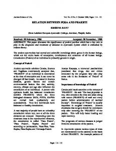
simulations is defined by projection on the ERA-40 regimes (cf. previous section), we checked that in this case the weather regime patterns still do not change between the present and future conditions. Indeed, Table 1 shows that for all four weather regimes the correlation between the present and future patterns obtained by projection on the ERA-40 regimes lies within the 90% confidence interval. Before verifying if the relationship between the weather regimes and the local temperature holds in the warmer climate, we first analyze the mean temperature change. Figure 3a shows the mean temperature change in 2070–99 with respect to 1970–99 for the entire winter season. The mean warming is not homogeneous: it follows an eastward gradient with a maximum in the northeast of Europe and a minimum in the North Atlantic. Because we apply the weather regime approach, it is important to assess which part of this total winter change is due to the modification of regimes. We have shown that the weather regime patterns do not change in the future. We now verify how their occurrence frequencies change. Table 2 illustrates the change in the frequency of occurrence between present and future climate. The significance of the change was estimated using bootstrap method.1 Only the change in the frequency of the blocking regime is significant at the 10% level. To evaluate which part of the total change in local winter temperature can be explained by changes in regime occurrence frequencies we used a linear decomposition (Boe´ et al. 2006; Najac et al. 2009), 4
DX 5 X
F
P
X 5
å ( f Fk xkF
k51
f Pk xkP ) 1 ( f F0 Y F
f P0 Y P ), (1)
where D X is the total change of temperature between the present and future climate, XP (XF) is the mean value of temperature in the present (future) climate scenario, 1 The method consists of creating an M-yr randomized dataset of geopotential height (M is randomly chosen to be between 2 and 50) by scrambling in the time domain the 50-yr data from the present climate simulation. The frequency of each of the four weather regimes was then estimated for the scrambled dataset. The same procedure of scrambling the original data was repeated 1000 times, which allows derivation of the PDF for the weather regime frequencies. The distribution is then used to assess the significance level.
1 JULY 2010
3757
NOTES AND CORRESPONDENCE
FIG. 3. (a) Mean winter temperature change (8C) in 2070–99 relative to 1970–99 for the entire winter season. (b)–(d) The corresponding changes inside the four weather regimes are shown as the anomalies from (a).
f Pk (f Fk ) is the frequency of occurrence for kth regime in the present (future) climate, xPk (x Fk ) is the mean temperature for kth regime for the present (future) simulation, f0P(f0F ) is the frequency of occurrence of the transition days in the present (future) climate, and YP(YF) is the mean temperature for the transition days for the present (future) simulation. Equation (1) can be rewritten as 8 9 < 4 = DX 5 [f Pk (xFk xPk )] 1 f P0 (Y F Y P ) :k51 ;
å
8 < 4 [xP ( f F 1 :k51 k k
å
2
14
f Pk )] 1 Y P ( f F0
;
4
å (xFk
k51
xPk )(f Fk
f P0 )
9 =
f Pk ) 1 (Y F
Y P )(f F0
3
f P0 )5. (2)
The first term of Eq. (2) is the ‘‘intratype’’ anomalies. It represents the part of the total change that is due to modifications within the weather regimes. The second term is the ‘‘intertype’’ anomaly, which shows the part of the change that is due to changes in occurrence frequency. The third term is a mixing term, which includes both intertype and intratype changes. We apply this decomposition to the temperature change averaged over central Europe (the region indicated by
a rectangle on the Fig. 3a). The results are reported in Table 3. The temperature change that is due to the intratype modification, or, in other words, the modification associated with the change in the link between the weather regime and regional temperature, considerably exceeds the temperature change resulting from the two other terms of the decomposition. Therefore, we only analyze the change in mean temperature within each regime (xFk 2 xPk ). Figures 3b–e show the changes for the zonal regime, Atlantic Ridge, blocking, and Greenland anticyclone, respectively. They are presented as anomalies from the whole winter changes of Fig. 3a. A positive anomaly thus means a stronger-thanaverage warming in that regime; a negative anomaly means a weaker warming. The magnitude of the temperature change in the zonal regime is close to the one for the entire winter (the anomalies are close to zero). The warming is less pronounced than average for the days corresponding to the Atlantic
TABLE 2. Weather regime occurrences (%) in the present and future climate simulation of LMDZ. Weather regimes for the model are obtained by projection on the observed weather regimes. Only the change in frequency of blocking regime is significant at the 10% level.
Present Future
ZO
AR
BL
GA
18 17
18 16
9 11
11 10
3758
JOURNAL OF CLIMATE
TABLE 3. Effects of the different terms on the mean temperature change (8C) between the periods 2070–99 and 1970–99 averaged over the region indicated by a rectangle on the Fig. 3a. Contribution of four weather regimes (ZO, AR, BL, and GA) and transition days (trans), and the total effect of each term (sum) are shown.
Intertype Intratype Mixing
ZO
AR
BL
GA
Trans
Sum
20.03 0.50 20.03
0.01 0.47 20.06
20.03 0.22 0.06
0.01 0.55 20.02
0.00 1.34 0.04
20.04 3.08 20.01
Ridge and the blocking, especially over eastern Europe. The Greenland anticyclone, in contrast, is characterized by an important temperature increase (up to 48C more than the average for winter). This last result could be related to the fact that in a warmer climate the minimum temperature increases faster than the maximum temperature (Solomon et al. 2007). Because the Greenland anticyclone is favorable for cold conditions over most of Europe, it is associated with the largest warming. Thus, the future temperature changes have different amplitudes among the four weather regimes. Are these differences large enough to change the most favorable regime for either warm or cold temperature over a given region? The dominant weather regimes for extreme warm and cold temperatures relative to the future mean are shown in Fig. 2 (bottom). The warm temperatures (Fig. 2e) are generally characterized by the same link with the large-scale circulation as in the control simulation. However, the relationship between the weather regimes and cold temperatures (Fig. 2f) is altered in the future. The influence of the Greenland anticyclone is weaker over a large part of Europe. It gives way to the Atlantic Ridge in the southwest and northeast, whereas in central Europe the blocking takes over. To consider the change found over central Europe in more detail, we use box-and-whisker plots to represent the statistical distribution of temperature variability.
VOLUME 23
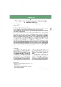
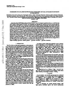
The boxes and whiskers denote the 5th, 25th, 50th, 75th, and 95th quantiles of the daily temperature distributions. Figure 4 shows daily temperatures averaged over the region indicated by a rectangle in Figs. 2d,f. Figure 4a corresponds to the present-day climate and Fig. 4b represents the future climate. The wide box-and-whisker plots denote the daily temperature distributions for the entire winter season (white box plot) and for the four weather regimes (colored box plots). In both the present and future climates, the zonal regime (red) corresponds to the warmest winter temperatures, and the blocking (blue) and Greenland anticyclone (yellow) are associated with temperatures that are lower than that of the entire season. The coldest temperatures occur during the Greenland anticyclone in the present climate. In the future, the temperature distribution for this regime is significantly shifted to higher values so that the temperature during the blocking regime is colder than the temperature during the Greenland anticyclone. This change can be explained as follows. In the presentday climate the Greenland anticyclone is favorable to low temperature in winter, because during this weather regime the westerlies are weakened and the temperature over the north of Europe is dominated by advection of cold air coming from the continent. In the future, the Greenland anticyclone is still associated with advection of continental air masses. However, because the future warming is, on average, more pronounced over the continental region (Fig. 3a), the advected air masses are less cold (relative to the local temperature) in the future than in the present-day climate.
7. Conclusions To analyze the link between the large-scale circulation and the European mean temperature, we use a qualitative relationship defined in terms of weather regimes that are most favorable for warm/cold temperatures. The
FIG. 4. Box-and-whisker plots of the daily mean temperature distribution (8C) in (a) 1970–99 and (b) 2070–99 over the region indicated by a rectangle in Figs. 2d,f. Wide white box represents the entire winter season distribution and colored boxes show the distributions inside the four weather regimes. The horizontal line within the box is the median; bottom and top box bounds show the 25th and 75th percentiles, respectively; bottom and top whisker bounds indicate the 5th and 95th percentiles, respectively. Color legend is as in Fig. 2.
1 JULY 2010
NOTES AND CORRESPONDENCE
technique of a favorable regime is a compact way to describe the change of the impact of the regimes on local temperature variability. The stability of the relationship is tested in the A2 climate scenario (2070–99) relative to the present conditions (1970–99), as simulated by LMDZ. We show that despite the absence of change in the regimes’ structures, their impact on the temperature distribution over central Europe changes in a warmer climate. Moreover, this change cannot be explained by changes in the occurrence frequencies of weather regimes, but rather it is due to the different amplitudes of warming among the four weather regimes. As a consequence, the relationship between the local temperature and the large-scale circulation is different in the present and in the future climates. The apparent cause is the future change in the mean temperature gradient, with a stronger warming over the continent; the consequences of anomalous advection in different circulation regimes are then different from the present. The basic hypothesis of statistical downscaling is thus not always valid in our case. This result suggests caution in using statistical downscaling techniques to predict local climate changes for impact studies. Acknowledgments. Computer resources were allocated by the IDRIS, the computer center of CNRS. The boundary conditions for LMDZ were extracted from the outputs of the IPSL global coupled model kindly provided by Jean-Louis Dufresne and Laurent Fairhead. Diagnostics were done with the R package (http://www. r-project.org). Authors thank the two anonymous reviewers for their constructive comments helped to improve this manuscript. REFERENCES Berner, J., and G. Branstator, 2007: Linear and nonlinear signatures in the planetary wave dynamics of an AGCM: Probability density functions. J. Atmos. Sci., 64, 117–136. Boe´, J., L. Terray, F. Habets, and E. Martin, 2006: A simple statisticaldynamical downscaling scheme based on weather types and conditional resampling. J. Geophys. Res., 111, D23106, doi:10.1029/2005JD006889. Cassou, C., L. Terray, and A. Phillips, 2005: Tropical Atlantic influence on European heat waves. J. Climate, 18, 2805–2811. Christiansen, B., 2005: Bimodality of the planetary-scale atmospheric wave amplitude index. J. Atmos. Sci., 62, 2528–2541. Corti, S., F. Molteni, and T. N. Palmer, 1999: Signature of recent climate change in frequencies of natural atmospheric circulation regimes. Nature, 398, 799–802. D’Andrea, F., and Coauthors, 1998: Northern Hemisphere atmospheric blocking as simulated by 15 atmospheric general circulation models in the period 1979–1988. Climate Dyn., 14, 385–407. Dufresne, J.-L., L. Fairhead, H. Le Treut, M. Berthelot, L. Bopp, P. Ciais, P. Friedlingstein, and P. Monfray, 2002: On the
3759
magnitude of positive feedback between future climate change and the carbon cycle. Geophys. Res. Lett., 29, 1405, doi:10.1029/ 2001GL013777. Efron, B., and R. Tibshirani, 1993: An Introduction to the Bootstrap. Statistics and Applied Probability, Vol. 57, Chapman and Hall/CRC, 456 pp. Goubanova, K., and L. Li, 2006: Extremes in temperature and precipitation around the Mediterranean basin in an ensemble of future climate scenario simulations. Global Planet. Change, 57, 27–42. Houghton, J. T., Y. Ding, D. J. Griggs, M. Noguer, P. J. van der Linden, X. Dai, K. Maskell, and C. A. Johnson, Eds., 2001: Climate Change 2001: The Scientific Basis. Cambridge University Press, 881 pp. Hourdin, F., and Coauthors, 2006: The LMDZ4 general circulation model, 2005: Climate performance and sensitivity to parameterized physics with emphasis on tropical convection. Climate Dyn., 19, 3445–3482. Hurrell, J., Y. Kushnir, G. Ottersen, and M. Visbeck, Eds., 2003: The North Atlantic Oscillation: Climatic Significance and Environmental Impact. Geophys. Monogr., Vol. 134, Amer. Geophys. Union, 279 pp. Huth, R., 1999: Statistical downscaling in central Europe: Evaluation of methods and potential predictors. Climate Res., 13, 91–101. Kimoto, M., and M. Ghil, 1993: Multiple flow regimes in the Northern Hemisphere winter. Part II: Sectorial regimes and preferred transitions. J. Atmos. Sci., 50, 2645–2673. Klein Tank, A., and Coauthors, 2002: Daily dataset of 20-century surface air temperature and precipitation series for the European Climate Assessment. Int. J. Climatol., 22, 1441–1453. Legras, B., and M. Ghil, 1985: Persistent anomalies, blocking, and variations in atmospheric predictability. J. Atmos. Sci., 42, 433–471. Majda, A. J., C. L. Franzke, A. Fischer, and D. T. Crommelin, 2006: Distinct metastable atmospheric regimes despite nearly Gaussian statistics: A paradigm model. Proc. Natl. Acad. Sci. USA, 103, 8309–8314. Michelangeli, P., R. Vautard, and B. Legras, 1995: Weather regimes: Recurrence and quasi-stationarity. J. Atmos. Sci., 52, 1237–1256. Najac, J., J. Boe´, and L. Terray, 2009: A multi-model ensemble approach for assessment of climate change impact on surface winds in France. Climate Dyn., 32, 615–634, doi:10.1007/ s00382-008-0440-4. Palmer, T. N., 1999: A nonlinear dynamical perspective on climate change. J. Climate, 12, 575–591. Plaut, G., E. Schuepbach, and M. Doctor, 2001: Heavy precipitation events over a few Alpine sub-regions and the links with largescale circulation, 1971-1995. Climate Res., 17, 285–302. Sanchez-Gomez, E., and L. Terray, 2005: Large-scale atmospheric dynamics and local intense precipitation episodes. Geophys. Res. Lett., 32, L24711, doi:10.1029/2005GL023990. Schubert, S., 1998: Downscaling local extreme temperature changes in south-eastern Australia from the CSIRO Mark2 GCM. Int. J. Climatol., 18, 1419–1438. Solomon, S., D. Qin, M. Manning, Z. Chen, M. Marquis, K. B. Averyt, M. Tignor, and H. L. Miller, Eds., 2007: Climate Change 2007: The Physical Science Basis. Cambridge University Press, 996 pp. Stephenson, D. B., A. Hannachi, and A. O’Neill, 2004: On the existence of multiple climate regimes. Quart. J. Roy. Meteor. Soc., 130, 583–606.
3760
JOURNAL OF CLIMATE
Tibaldi, S., and F. Molteni, 1990: On the operational predictability of blocking. Tellus, 42A, 343–365. Uppala, S., and Coauthors, 2005: The ERA-40 Re-Analysis. Quart. J. Roy. Meteor. Soc., 131, 2961–3012. Vautard, R., 1990: Multiple weather regimes over the North Atlantic: Analysis of precursors and successors. Mon. Wea. Rev., 118, 2056–2081. von Storch, H., and F. W. Zwiers, 2001: Statistical Analysis in Climate Research. Cambridge University Press, 484 pp. Wilby, R., S. Charles, E. Zorita, B. Timbal, P. Whetton, and L. Mearns, 2004: Guidelines for use of climate scenarios developed from
VOLUME 23
statistical downscaling methods. Data Distribution Centre of the IPCC Tech. Rep., 27 pp. [Available online at http://www. ipcc-data.org/guidelines/dgm_no2_v1_09_2004.pdf.] Yiou, P., and M. Nogaj, 2004: Extreme climatic events and weather regimes over the North Atlantic: When and where? Geophys. Res. Lett., 31, L07202, doi:10.1029/ 2003GL019119. ——, K. Goubanova, L. X. Li, and M. Nogaj, 2008: Weather regime dependence of extreme value statistics for summer temperature and precipitation. Nonlinear Processes Geophys., 15, 365–378.