Relation Extraction Using Support Vector Machine

Relation Extraction Using Support Vector Machine Gumwon Hong University of Michigan, Ann Arbor, MI 48109 [email protected]

Abstract. This paper presents a supervised approach for relation extraction. We apply Support Vector Machines to detect and classify the relations in Automatic Content Extraction (ACE) corpus. We use a set of features including lexical tokens, syntactic structures, and semantic entity types for relation detection and classification problem. Besides these linguistic features, we successfully utilize the distance between two entities to improve the performance. In relation detection, we filter out the negative relation candidates using entity distance threshold. In relation classification, we use the entity distance as a feature for Support Vector Classifier. The system is evaluated in terms of recall, precision, and Fmeasure, and errors of the system are analyzed with proposed solution.

1 Introduction The goal of Information Extraction (IE) is to pull out pieces of information that are salient to the user’s need from large volume of text. With the dramatic increase of World Wide Web, there has been growing interest in extracting relevant information from large textual documents. The IE tasks may vary in detail and reliability, but two subtasks are very common and closely related: named entity recognition and relation extraction. Named entity recognition identifies named objects of interest such as person, organizations or locations. Relation extraction involves the identification of appropriate relations among these entities. Examples of the specific relations are employee-of and parent-of. Employee-of relation holds between a particular person and a certain organization and parent-of holds between a father and his child. According to Message Understanding Conferences (MUC), while named entities can be extracted with 90% or more in F measure with a state of the art system, relation extraction was not so successful [8]. In this paper we propose a supervised machine learning approach for relation extraction. The goal of this paper is to investigate an empirical method to find out useful features and experimental procedure to increase the performance of relation extraction. We divide the extraction task into two individual subtasks: relation detection and relation classification. Relation detection is involved in identifying from every pair of entities positive examples of relations which can fall into one of many relation categories. In relation classification, we assign a specific class to each detected relation. To each task, we apply distinct linguistic features ranging from lexical tokens to syntactic structures as well as the semantic type information of the entities. We also applied the distance between two entities to make the detection problem easier and to increase the R. Dale et al. (Eds.): IJCNLP 2005, LNAI 3651, pp. 366 – 377, 2005. © Springer-Verlag Berlin Heidelberg 2005

Relation Extraction Using Support Vector Machine

367

performance of both the relation detection and classification. We apply Support Vector Machines (SVMs) partly because it represents the state of the art performance for many classification tasks [3]. As we will discuss in section 3 about features, we are working on very high dimensional feature space, and this often leads to overfitting. Thus, the main reason to use SVMs is that this learning algorithm has a robust rationale for avoiding overfitting [11]. This paper is structured in the following manner. In section 2, we survey the previous work on relation extraction with emphasis on supervised machine learning approaches. In section 3, the problem formalization, the description of dataset and the feature extraction methods will be discussed. In section 4, we conduct a performance evaluation of the proposed approach and error analysis on ACE dataset. Finally, in section 5, a conclusion and discussion of future work will be followed.

2 Related Work Relation extraction was formulated as part of Message Understanding Conferences (MUC) [8], which has focused on a series of information extraction tasks, including analyzing free text, recognizing named entities, and identifying relations of a specified type. Work on relation extraction over the last two decades has progressed from linguistically unsophisticated models to the adaptation of NLP techniques that use shallow parsers or full parsers and complicated machine learning methods. [7] addressed the relation extraction problem by extending the statistical parsing model which simultaneously recovers syntactic structures, named entities, and relations. They first annotated sentences for entities, descriptors, coreference links and relation links, and trained the sentences from Penn Treebank. Then they applied to new training sentences and enhanced the parse trees to include the IE information. Finally they re-retrained the parser on newly enriched training data. More recently, [12] introduced the kernel methods to extract relations from 200 news articles from different publications. The kernels are defined over shallow parse representations of text and computed through a dynamic programming fashion. They generated relation examples from shallow parses for two relations: person-affiliation and organization-location. Performance of the kernel methods was compared with feature-based methods and it showed that kernels have promising performance. [4] extended work in [12] to estimate kernel functions between augmented dependency trees. Their experiment has two steps. Relations were first detected and then classified in cascading manner. However, the recall was relatively low because many positive examples of relations were dropped during detection phase. Detecting relations is hard job for kernel methods because, in detection, all negative examples are heterogeneous and it is difficult to use similarity function. [13] proposed weakly supervised learning algorithm for classifying relations in ACE dataset. He introduced feature extraction methods for his supervised approach as well as a bootstrapping algorithm using random feature projection (called BootProject) on top of SVMs. He compared BootProject with supervised approach, and showed that BootProject algorithm reduced much work needed for labeling training data without decreasing the performance.

368

G. Hong

Our approach to relation extraction adapts some feature extraction methods from [13] but differs from [13] in two important aspects. First, instead of only classifying relations by assuming all candidate relations are detected, we perform relation detection before classifying relations by regarding every pair of entities in a sentence as a target of classification. Second, we used total 7652 (6140 for training and 1512 for development testing) relation examples in ACE dataset, but in [13] only 4238 relations were used for training and 1022 for testing. We increase the performance by using more training data and reducing errors in data processing stage.

3 Data Processing 3.1 Problem Definition Our task is to extract relations from unstructured natural language text. Because we determine the relationship for every pair of entities in a sentence, our task is formalized with a standard classification problem as follows: (e1 ,e2, s) → r where e1 and e2 are two entities existing in sentence s, and r is a label of the relation. Every pair of entities in a sentence can be a relation or not, so we call the triple (e1, e2, s) a relation candidate. With the possible set of values of r, there can be at least three tasks. 1. Detection only: For each relation candidate, we predict whether it constitutes an actual relation or not. In this task, a label r can be either +1 (two entities are related) or -1 (not related). 2. Combined detection and classification: For each relation candidate, we perform N+1 way classification, where N is the number of relation types. Five relation types are specified in next subsection. The additional class is -1 (two entities are not related). 3. Classification only: For each relation, we perform N way classification. In this task, we assume that all relation candidates in test data are manually labeled with N+1 way classification. We only consider the classifier’s performance on the N relation types. We use a supervised machine learning technique, specifically Support Vector Machine classifiers, and we empirically evaluate the performance in terms of recall, precision and F measure. To make the problem more precisely, we constrain the task of relation extraction with following assumptions: 1. Entities should be tagged beforehand so that all information regarding entities is available when relations are extracted. 2. Relations are binary, i.e., every relation takes exactly two primary arguments. 3. The two arguments of a relation, i.e., an entity pair, should explicitly occur within a sentence. 4. Evaluation is performed over five limited types of relations as in Table 1.


369

A relation is basically an ordered pair, thus “Sam was flown to Canada” contains the relation AT(Sam, Canada) but not AT(Canada, Sam). However, 7 relations in NEAR (relative location) and SOCIAL (associate, other-personal, other-professional, other-relative, sibling, and spouse) types are symmetric. For example, the sentences such as ”Bill is the neighbor of Sarah.” and “The park is two blocks from Walnut Street” do not distinguish the order of entities. Table 1. Relation types and their subtypes in ACE 2 corpus BASED-IN, LOCATED, RESIDENCE RELATIVE-LOCATION OTHER, PART-OF, SUBSDIARY AFILIATE-PARTNER, CITIZEN-OF, CLIENT, FOUNDER, GENERAL-STAFF, MANAGEMENT, MEMBER, OTHER, OWNER SOCIAL ASSOCIATE, GRANDPARENT, OTHER-PERSONAL, OTHER-PROFESSIONAL, OTHER-RELATIVE, PARENT, SIBLING, SPOUSE

AT

NEAR PART ROLE

3.2 Data Set We extract relations from the Automatic Content Extraction (ACE) corpus, specifically version 1.0 of the ACE 2 corpus, provided by the National Institute for Standards and Technology (NIST). ACE corpora consist of 519 annotated text documents assembled from a variety of sources selected from broadcast news programs, newspapers, and newswire reports [1]. According to the scope of the LDC ACE program 1, current research in information extraction has three main objectives: Entity Detection and Tracking (EDT), Relation Detection and Characterization (RDC), and Event Detection and Characterization (EDC). This paper focuses on the second sub-problem, RDC. For example, we want to determine whether a particular person is at certain location, based on the contextual evidence. According to the RDC guideline version 3.6, Entities are limited to 5 types (PERSON, ORGANIZATION, GEO-POLITICAL ENTITY (GPE), LOCATION, and FACILITY), and relations are also classified into 5 types: Role: Role relations represent an affiliation between a Person entity and an Organization, Facility, or GPE entity. Part: Part relations represent part-whole relationships between Organization, Facility and GPE entities. At: At relations represent that a Person, Organization, GPE, or Facility entity is located at a Location entity. Near: Near relations represent the fact that a Person, Organization, GPE or Facility entity is near (but not necessarily “at”) a Location or GPE entity. Social: Social relations represent personal and professional affiliations between Person entities. Table 1 lists the 5 major relation types and their subtypes. The numbers in the bottom row indicate the number of instances in training data and development testing data. We do not classify the 24 subtypes of relations due to the sparse instances of many subtypes.

370

G. Hong

Table 2. Breakdown of the ACE dataset (#f and #r means number of files and number of relations respectively) Training data #f #r 325 4628

Held-out data #f #r 97 1512

#f 97

Test data #r 1512

Table 2 shows the breakdown of the ACE dataset for our task. Training data takes about 60% of all ACE corpora, and each held-out data and test data contains about 20% of the whole distribution in the number of files as well as in the number of relations.1 3.3 Data Processing We start with entity marked data and the first step is to detect the sentence boundary using the sentence segmenter provided by DUC competition2. Performance of the sentence segmentater is crucial for relation detection because the number of entity pairs combinatorially increases as a sentence grows in size. The original DUC segmenter fails to detect sentence boundary if the last word of a sentence is a named entity and annotated with brackets, i.e., ‘’. We modified the DUC segmenter by adding simple rules where we mark sentence boundary if every bracket is followed by ‘?’, ‘!’, or ‘.’. At this step, we drop the sentences if the sentence has less than two entities. Sentence parsing is then performed using Charniak parser [6] on these target sentences in order to obtain the necessary linguistic information. To facilitate the feature extraction, parse trees are converted into chunklink format [2]. Chunklink format contains the same information as the original parse tree, but it provides for each word the chunk to which it belongs, its grammatical function, grammatical structure hierarchy, and trace information. 3.4 Features We are ready to introduce our feature sets. The following features include lexical tokens, part of speech, syntactic features, semantic entity types, and the distance between two entities (we will say “entity distance” to refer to distance between two entities in the remaining part of this paper). These features are selectively used for three tasks defined in section 3.1. 1. Words. Lexical token of both entity mentions3 as well as all the words between them. If two or more words constitute an entity, each individual word in an entity is a separate feature. 2. Part of speech. Part of speech corresponding to each word feature described above. 1

2 3

Training data and held-out data together are called "train", and test data is called "devtest" in the ACE distribution. http://duc.nist.gov/past_duc/duc2003/software/ Entities are objects and they have a group of mentions, and the mentions are textual references to the objects.


371

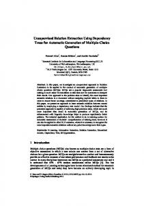
3. Entity type. Entities have one of five types (person, location, organization, geopolitical entity, or facility). 4. Entity mention type. An entity mention can be named, nominal, or pronominal. Entity mention type is also called the level of a mention. 5. Chunk tag. A word is inside (I), outside (O) or in the beginning (B) of a chunk. A chunk here stands for a standard phrase. Thus, the word “George” at the beginning of NP chunk “George Bush” has B-NP tag. Similarly, the word “named” has I-VP tag in VP chunk “was named”. 6. Grammatical function tag. If a word is the head word of a chunk, it has function of whole chunk. The other words in a chunk that are not the head have "NOFUNC" as their function. For example, the word “task” is head of NP chunk “the task” and it has grammatical function tag “NP”, while “the” has “NOFUNC”. 7. IOB chain. The syntactic categories of all the constituents on the path from the root node to the leaf node of a parse tree. For example, a word’s IOB chain I-S/I-NP/B-PP means that it is inside a sentence, inside a NP chunk, and in the beginning of PP chunk. 8. Head word Path. The head word sequence in the path between two entity mentions in the parse tree. This feature is used after removing duplicate elements. 9. Distance. The number of words between two entity mentions. 10. Order. Relative position of two relation arguments. Two entities and all words between them have separate features of chunk tags (5), grammatical function tags (6), and IOB chains (7), and these three features are all automatically computed by chunklink.pl. See [2] for further description of these three terminologies. We use the same method as in [13] to use the features described in 3, 5, 6, 7, and 10. The concept of the head word path is adapted from [10]. Let us take a sentence “Officials in New York took the task” for an example. Two entity mentions, officials and New York, constitute a relation AT(officials, New York). For the noun phrase “officials in New York”, the corresponding parse tree is shown in Fig 2. To compute the head word path, we need to know what a head word is. At the terminal nodes, the head word is simply the word from the sentence the node represents. At non-terminal nodes in the parse tree, “The head of a phrase is the element inside the phrase whose properties determine the distribution of that phrase, i.e. the environments in which it can occur.” [9] The head word path is computed in the following way. The head words of the two entity mentions are officials and York respectively. The path between these two head words is the sequence officials-NP-PP-NP-York which is in bold in Fig. 1. Then we change each non-terminal into its head word, and we get officials-officials-in-YorkYork. If we remove the duplicate elements, we get officials-in-York. Finally, we replace the two entity mentions with their entity mention types, resulting in PERSONin-GPE.

372

G. Hong

NP PP NP

NNS Officials

IN in

NNP New

NNP York

took

…

Fig. 1. Parse tree for the fragment “officials in New York”. The path between two entity mentions is in bold.

Table 3 shows the features for the noun phrase “officials in New York”. Note that all features are binary and they are assigned 1 or -1 depending on whether an example contains the feature or not. We could have n+1 possible distance features, where n is the entity distance threshold. Table 3. Example of features for Officials in New York. e1 and e2 are two entities that constitute a relation AT(officials, New York). Features

Example

Words Part-of-speech Entity type Entity mention type Chunk tag Grammatical function tag

officials(e1), in, New(e2-1), York(e2-2) NNS(e1), IN, NNP(e2-1), NNP(e2-2) officials: PERSON, New York: GPE officials: NOMINAL, New York: NAME B-NP, B-PP,B-NP, I-NP NP, PP, NOFUNC, NP officials: B-S/B-NP/B-NP, in: I-S/I-NP/B-PP, New: I-S/I-NP/I-PP/B-NP York: I-S/I-NP/I-PP/I-NP PERSON-in-GPE Distance=1 e1 before e2

IOB chain Head word path Distance Order

Besides the linguistic features, we apply entity distance to each task. When detecting actual relations, we use the entity distance to filter the unnecessary examples. To achieve the optimal performance, we set a threshold to keep the balance between recall and precision. We choose the threshold of entity distance based on the detection performance on held-out data. When classifying the individual relation types, the entity distance is also successfully used as a feature. We will discuss how the entity distance is utilized as a feature in the next section. When performing combined detection and classification, we use two-staged extraction: we first detect relations in the same way as detection only task, and then perform classification on detected relations to predict the specific relation types. There are two important reasons that we choose this two-staged extraction.


373

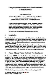
First, we detect relations to increase the recall for whole extraction task. Because every combination of two entities in a sentence can construct a relation, we have far more negative examples of relation4 in our training data. If we perform single-staged N+1 classification, the classifier is more likely to identify a testing instance as a nonrelation because of the disproportionate size in samples which often decreases the performance. Thus in detection stage (or detection only task), we perform binary classification by enriching our training samples by assuming 5 types of relations to be one positive class. Second, before performing relation classification, we can reduce a significant number of negative examples with only limited sacrifice of the detection performance by using a filtering technique with entity distance threshold. Fig. 2 shows the positive and negative examples distributed over the entity distances in training data. As we can see from the positive example curve (lower curve in the graph), the number of positive examples decreases as the entity distance exceeds 1. Positive examples do not exist where the entity distance is more than 32, while negative examples can have entity distances more than 60. 7000

6000 negative example positive example

# examples

5000

4000

3000

2000

1000

0 0

5

10

15

20

25

30

35

40

45

50

55

60

distance between entities

Fig. 2. Distribution of samples over entity distances in training data

We can also discover that almost 99% of the positive examples are distributed below the entity distance 20. If we restrict an entity distance threshold to 5, that is if we remove samples whose entity distances are more than 5, then whereas 71% of negative examples are dropped out, we can still maintain 80% of the positive examples. As can be seen in the graph, negative relations take more than 95% of whole entity pairs. This class imbalance makes the classifier less likely to identify a testing instance as a relation. The threshold makes relation detection easier because we can remove the large portion of negative examples, and we can get the result in reasonable time. 4

We have total 6551 positive relation examples out of 131510 entity pairs in training data.

374

G. Hong

In our experiment we tested the following 3 sets of features: F1: words + entity type + entity mention type + order F2: F1 + all syntactic features (2, 5, 6, 7 and 8) F3: F2 + distance F1 is the set of simple features that can be obtained directly from the ACE corpus without applying any NLP techniques. Features in F2 require sentence boundary detection and parsing to acquire the syntactic structure of a sentence. F3 is used to determine whether an entity distance can be successfully used for our task.

4 Experiments and Error Analysis We applied Support Vector Machines (SVMs) classifier to the task. More specifically, we used LIBSVM with RBF (Radial Basis Function) kernel [3]. SVMs attempt to find a hyperplane that split the data points with maximum margin, i.e., the greatest distance between opposing classes [11]. The system performance is usually reflected using the performance measures of information retrieval: precision, recall, and F-measure. Precision is the ratio of the number of correctly predicted positive examples to the number predicted positive examples. Recall is the ratio of the number of correctly predicted positive examples to the number of true positive examples. F-measure combines precision and recall as follows: F-measure = 2 * precision * recall / (precision + recall) We report precision, recall, and F-measure for each experiment. We use different features for relation detection and relation classification. In relation detection, which is either in detection only task or in the first stage of combined detection and classification, we do not use entity distance as a feature. Instead, we get rid of the negative examples of relations by setting a threshold value of the entity distances. The threshold is chosen in a way that we could achieve the best F-measure score of relation detection performance on held-out data with a classifier trained on training data. We have fixed the entity distance threshold to be 7 by this experiment, and this threshold enables us to remove 67% of the negative examples and keep 93% of the positive example. We will use this value in the remaining experiments. In relation classification, which is either in the second stage of combined extraction or in classification only task, we use all the features described in Table 3. Entity distance is successfully used as a feature to classify the individual relation types. Let us take a relation type NEAR for an example to see why entity distance is useful. As shown in table 4, the average entity distance of NEAR relations is relatively greater than the average distances of any other types of relations. Table 4. Average entity distance for 5 relation types in training data. The first row indicates the average entity distances over the relations whose entity distances are less than or equal to 7. Relation Avg Entity distance (