QSVM: A Support Vector Machine For Rule Extraction Guido Bologna1 and Yoichi Hayashi2 1
University of Applied Sciences of Western Switzerland, Rue de la Prairie 4, Geneva 1202, Switzerland,
[email protected], 2 Meiji University, Dept. of Computer Science, Tama-ku, Kawasaki, Kanagawa 214-8571, Japan
[email protected]
Abstract. Rule extraction from neural networks represents a difficult research problem, which is NP-hard. In this work we show how a special Multi Layer Perceptron architecture denoted as DIMLP can be used to extract rules from ensembles of DIMLPs and Quantized Support Vector Machines (QSVMs). The key idea for rule extraction is that the locations of discriminative hyperplanes are known, precisely. Based on ten repetitions of stratified 10-fold cross validation trials and with the use of default learning parameters we generated symbolic rules from five datasets. The obtained results compared favorably with respect to another state of the art technique applied to Support Vector Machines. Keywords: Rule Extraction, Ensembles, SVM
1
Introduction
In various domain applications, explaining answers provided by neural network models is crucial. For instance a physician cannot trust any model without explanation. A natural way to elucidate the knowledge embedded within neural network connections is to extract symbolic rules. However, producing rules from Multi Layer Perceptrons (MLPs) is a NP-hard problem [12]. Since the earliest work of Gallant on rule extraction from neural networks [11], many techniques have been introduced. In the nineties Andrews et al. introduced a taxonomy to characterize rule extraction techniques [1]. Later, Duch et al. published a survey article on this topic [10]. Finally, Diederich et al. published a book on techniques to extract symbolic rules from Support Vector Machines (SVMs) [9] and Barakat and Bradley reviewed a number of rule extraction techniques applied to SVMs [2]. More than twenty years ago Hansen and Salamon demonstrated that combining several neural networks in an ensemble can improve the predictive accuracy with respect to a single model [13]. Nevertheless, only a few authors started to extract rules from neural network ensembles. Bologna proposed the Discretized
2
Interpretable Multi Layer Perceptron (DIMLP) to produce unordered symbolic rules from both single networks and ensembles [5]. With the DIMLP architecture rule extraction is performed by determining the precise location of axisparallel discriminative hyperplanes. Zhou et al. introduced the REFNE algorithm (Rule Extraction from Neural Network Ensemble) [19], which utilizes the trained ensembles to generate instances and then extracts symbolic rules from those instances. Attributes are discretized during rule extraction and it also uses particular fidelity evaluation mechanisms. Moreover, rules have been limited to only three antecedents. More recently Hara and Hayashi proposed the two-MLP ensembles by using the “Recursive-Rule eXtraction” (Re-RX) algorithm [17] for data with mixed attributes [14]. Re-RX utilizes C4.5 decision trees and backpropagation to train the MLPs recursively. Here, the rule antecedents for discrete attributes are disjointed from those for continuous attributes. Subsequently Hayashi at al. presented the “three-MLP Ensemble”by the Re-RX algorithm [15]. In this work we introduce the Quantized Support Vector Machine (QSVM), which is a novel DIMLP network trained by an SVM learning algorithm. This special architecture makes it possible to apply the rule extraction algorithm introduced in [5]. Based on stratified 10-fold cross validation trials, rules are generated and compared from both QSVMs and DIMLP ensembles on five datasets. Finally, we compare the accuracy and complexity of rules extracted from QSVMs with those generated in another work [16]. In the following sections we present the DIMLP model for which QSVM represents a particular case, the experiments, followed by the conclusion.
2
The DIMLP model
A symbolic rule is defined as: “if tests on antecedents are true then conclusion”; where “tests on antecedents” are in the form xi ≤ vi or xi ≥ vi ; with xi as an attribute value and vi as a real value. Generally, extracted rulesets are ordered or unordered. Ordered rules correspond to “if . . . then . . . else if . . . ” logical arrangement. Because of the presence of “else”, a rule implicitly negates the antecedents of the previous rule. Thus, with the exception of the first rule all the other rules depend also on a number of hidden antecedents corresponding to the negation of the previous antecedents. Unordered rules correspond to “if . . . then . . . ” structure. Contrary to ordered rules, a sample can activate more than one rule. Generally, unordered rulesets present more rules and antecedents, since all rule antecedents are explicitly displayed. The extraction of symbolic rules is based on a special MLP architecture. We first introduced the Interpretable Multi Layer Perceptron (IMLP) [3]. Later we presented the DIMLP model [5] and finally we demonstrated how to generate symbolic rules from DIMLP ensembles. The main novelty of this work consists in making it possible to transform a single DIMLP into a particular SVM network. Thus, the training is achieved by a typical SVM learning algorithm [18] and rule extraction is carried out by the same method used for DIMLPs. This new model is denoted as Quantized Support Vector Machine (QSVM).
3
2.1
IMLP networks
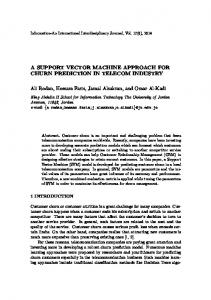
An IMLP differs from an MLP in the connectivity between the input layer and the first hidden layer. Specifically, any hidden neuron receives only a connection from an input neuron and the bias neuron, as shown in Figure 1.
y1 v0 = −2
1
x2
h1 = 0
h1 = 1
v1 = 3
h1 w0
1
w1
x1 −w0/w1 y1
v0 = −2
1
h1 = 0
h1 = 1
v1 = 1
h1 w0
1
x2
x1
w1
x1 −w0/w1
x1
Fig. 1. Example of simple IMLP networks. Depending on weight values v0 and v1 , at the top a discriminative hyperplane is created, but not at the bottom.
In addition, the activation function in the hidden layer is a threshold function. The output hk of the kth neuron of the first hidden layer is: { ∑ 1 if l wkl .xl > 0 (1) hk = 0 otherwise In the other layers the activation function is a sigmoid σ(x): σ(x) =
1 1 + exp(−x)
(2)
Note that the threshold activation function makes it possible to precisely locate possible discriminative hyperplanes. Specifically, in Figure 1 assuming two different classes, the first is being selected when y1 > 0.5 and the second with y1 ≤ 0.5. Hence, a possible hyperplane split could be located in −w0 /w1 . However, this hyperplane will result discriminative only when v1 > |v0 |. Another example is shown in figure 2. Weights v0 , v1 and v2 linearly separate white squares and black circles, since the possible values of h1 and h2 define a logical OR classification problem.
4
y1 x2 v0 = -10
h1 = 0 h2 = 1
h1 = 1 h2 = 1
h1 = 0 h2 = 0
h1 = 1 h2 = 0
v1 = 5 v2 = 6 -w20/w2
1
h1 w10
h2 w20
w1
w2
x1
1
x2
-w10/w1
x1
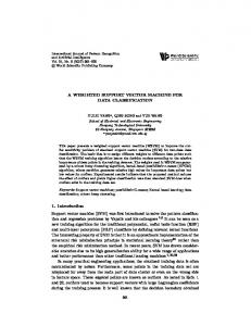
Fig. 2. An IMLP network creating two discriminative hyperplanes.
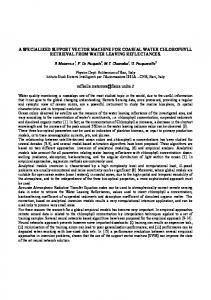
Figure 3 depicts an IMLP that will not be able to learn the classification problem represented in the right part of the figure. The reason is that weights between h1 , h2 and y1 cannot create two discriminative hyperplanes, since the possible values of h1 and h2 defines a logical XOR problem.
y1 x2 -w20/w2
1
h1 w10
h1 = 1 h2 = 1
h1 = 0 h2 = 0
h1 = 1 h2 = 0
w20
w1
1
h2
h1 = 0 h2 = 1
x1
w2
x2
-w10/w1
x1
Fig. 3. An IMLP network unable to correctly classify a problem of two classes.
2.2
DIMLP networks and ensembles
DIMLP networks represent a generalization of IMLPs. Essentially, they usually have two hidden layers, with the first one related to a stair activation function, instead of a threshold function. The stair function S(x) is given as If x < Rmin S(x) = σ(Rmin ) [ ] Rmax −Rmin x−Rmin )) If Rmin ≤ x ≤ Rmax (3) S(x) = σ(Rmin + d · Rmax −Rmin · ( d S(x) = σ(Rmax ) If x > Rmax
5
where σ is the sigmoid function, d is the number of stairs and Rmin and Rmax forms a range of d − 1 stairs. Finally, ”[]” denotes the integer part notation. Each neuron of the first hidden layer virtually creates a number of virtual parallel hyperplanes that is equal to the number of stairs of its stair activation function. As a consequence, the rule extraction algorithm corresponds to a covering algorithm for which the goal is to determine whether a virtual hyperplane is virtual or effective. A distinctive feature of this rule extraction technique is that fidelity, which is the degree of matching between network classifications and rules’ classifications is equal to 100%, with respect to the training set. Here we describe the general idea behind the rule extraction algorithm, since the details are provided in [6]. According to the 100% fidelity criterion, a decision tree is generated from the list of discriminative hyperplanes; then symbolic rules are extracted by simply following each path of the tree. At this point rules generally present too many antecedents; hence, a pruning process is carried out. Moreover, a “greedy” algorithm is performed in order to maximize the number of covered samples by modifying the thresholds of the antecedents. Overall, the computational complexity of the rule extraction algorithm is polynomial with respect to the number of stairs in the stair function, the number of inputs and the number of training samples. Ensembles of DIMLP networks can be trained by bagging [7] or arcing [8]. Bagging and arcing are based on resampling techniques. On one hand, assuming a training set of size p, bagging selects for each classifier included in an ensemble p samples drawn with replacement from the original training set. Hence, for each DIMLP network many of the generated samples may be repeated while others may be left out. On the other hand, arcing defines a probability with each example of the original training set. For each classifier the examples contained in the training set are selected according to these probabilities. Before learning all the training samples have the same probability to belong to a new training set (= 1/p). Then, after the first classifier has been trained the probability of sample selection in a new training set is increased for all unlearned samples and decreased for the others. Rule extraction from ensembles can still be performed, since an ensemble of DIMLP networks can be viewed as a single DIMLP network with one more hidden layer. For instance, in Figure 4 a “Transparent Box” corresponds to a single DIMLP that can be translated into symbolic rules. The linear combination is again a transparent box with one more layer of weights.
2.3
QSVM
The classification decision function of an SVM model is given by C(x) = sign(
∑ i
αi yi K(xi , x) + b);
(4)
6
Transparent Box
Majority Voting
Linear Combination
Non-Linear Combination
Fig. 4. Ensembling DIMLP networks by majority voting, linear combination and nonlinear combination.
αi and b being real values, yi ∈ {−1, 1} corresponding to the target values of the support vectors, and K(xi , x) representing a kernel function with xi as the vector components of the support vectors. The following kernels are used: – dot; – polynomial; – Gaussian. Specifically, for the dot and polynomial cases we have: K(xi , x) = (xi · x)d ;
(5)
with d = 1 for the dot kernel and d = 3 for the polynomial kernel. The Gaussain kernel is: K(xi , x) = exp(−γ||xi − x||2 );
(6)
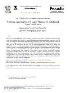
with γ > 0, a parameter. We define a Quantified Support Vector Machine (QSVM) as a DIMLP network with two hidden layers. The activation function of the neurons in the second hidden layer is related to the SVM kernel. For instance, with a dot kernel the corresponding activation function is the identity, while with a Gaussian kernel the activation function is Gaussian. The number of neurons in this layer is equal to the number of support vectors, with the incoming weight connections corresponding to the components of the support vectors. Figure 5 presents a QSVM with a Gaussian activation function in the second hidden layer. The activation function of the output neuron (only for classification problems of two classes) is a threshold function. Finally, neurons in the first hidden layer use a stair function.
7
Output Neuron b
uj
1
h’j
Wl0
1
hk
vjk
wkl xl
Input Layer
Fig. 5. A QSVM network.
Weights between the second hidden layer and the output neuron denoted as uj correspond to αj coefficients in equation 4. Moreover, a weight between the first and second hidden layers denoted as vjk corresponds to the j th component of the k th support vector. Finally, the role of neurons of the first hidden layer is to perform a normalization of the input attributes. Thus, during the training phase weights between the input layer and the first hidden layer remain unchanged. For clarity, let us assume that we have the same number of input neurons and hidden neurons in the first hidden layer. These weights are defined as: – wkl = 1/σl , with σl as the standard deviation of input variable l; – wl0 = −µl /σl , with µl as the average on the training set of the lth attribute. According to these weight values, when the stair function is a threshold function, neurons of the first hidden layer are activated with values 0 or 1, depending on whether the input attributes are greater than their corresponding average values µl . With an arbitrary number of stairs the activations of the first hidden layer will correspond to discrete values between 0 and 1. During training, weights above the first hidden layer are modified according to the SVM training algorithm [18]. After training, since QSVM is also a DIMLP network, rules can be extracted by performing the DIMLP rule extraction algorithm.
3
Experiments
In the experiments we used five datasets representing classification problems of two classes. Table 1 illustrates their main characteristics in terms of number of samples, number of input features, type of features, and source3 . All the 3
In this column UCI designates the Machine Learning Repository at the University of California, Irvine (www.archive.ics.uci.edu/ml/).
8
results are based on ten repetitions of stratified 10-fold cross-validation trials with normalized attributes and default learning parameters. Table 1. Datasets used in the experiments.
Dataset Name
Number of Samples Number of Inputs Attribute Types Ref.
Istambul Stock Exchange
536
8
Australian Credit Approval
690
14
Breast Cancer
683
9
discrete
UCI
Coronary Heart Disease
884
16
bool, real
[4]
Vertebral Column
310
6
real
UCI
3.1
real
bool, discr, real UCI
Models and learning parameters
The following models were trained on the five datasets: – – – – –
DIMLP ensembles trained by bagging (DIMLP-B); DIMLP ensembles trained by arcing (DIMLP-A); QSVM with dot kernel (QSVM-L); QSVM with polynomial kernel of third degree (QSVM-P3); QSVM with Gaussian kernel (QSVM-G).
Learning parameters were assigned to default values for both DIMLP ensembles and QSVMs. For DIMLP ensembles the learning parameters are: – – – –
the the the the
learning parameter η (η = 0.1); momentum µ (µ = 0.6); Flat Spot Elimination (F SE = 0.01); number of stairs q in the stair function (q = 50).
The default number of neurons in the first hidden layer is equal to the number of input neurons and the number of neurons in the second hidden layer is empirically defined in order to obtain a number of weight connections that is less than the number of training samples. Finally, the default number of DIMLPs in an ensemble is equal to 25, since it has been observed many times that for bagging and arcing the most substantial improvement in accuracy is achieved with the first 25 networks. In QSVMs the default learning parameters are those defined in the libSVM library4 . Here our goal was not to optimize the predictive accuracy of the models, but just to use default configurations and to determine how would vary accuracy and complexity of the models. 4
UCI
This software is available at http://www.csie.ntu.edu.tw/˜cjlin/libsvm/
9
3.2
Results
For all the models table 2 shows the average accuracy on the training set, while table 3 illustrates the average predictive accuracy. Table 2. Average accuracy on the training set. Dataset Name
DIMLP-B DIMLP-A QSVM-L QSVM-P3 QSVM-G
Istambul Stock Exchange
79.2 0.1
77.0 1.6
79.0 0.2
79.3 0.2
80.2 0.1
Australian Credit Approval
88.8 0.2
99.9 0.1
85.5 0.2
86.7 0.1
86.2 0.0
Breast Cancer
98.0 0.1
100.0 0.0
95.2 0.0
92.3 0.0
97.2 0.0
Coronary Heart Disease
95.9 0.1
100.0 0.0
87.1 0.1
88.3 0.1
87.8 0.1
Vertebral Column
88.2 0.2
95.2 0.7
86.0 0.1
86.8 0.3
85.6 0.2
90.0
94.4
86.6
86.7
87.4
AVERAGE
Table 3. Average predictive accuracy (on the testing sets). Dataset Name
DIMLP-B DIMLP-A QSVM-L QSVM-P3 QSVM-G
Istambul Stock Exchange
77.6 0.6
75.3 1.8
77.7 1.0
76.4 0.6
77.1 1.0
Australian Credit Approval
86.7 0.4
86.2 0.4
85.6 0.2
86.1 0.4
85.8 0.2
Breast Cancer
97.1 0.2
96.6 0.3
95.1 0.2
92.1 0.2
97.2 0.1
Coronary Heart Disease
93.1 0.4
94.6 0.6
86.3 0.3
87.5 0.2
86.9 0.2
Vertebral Column
85.5 0.8
84.2 1.1
84.9 0.4
85.0 0.9
84.4 0.7
88.0
87.4
85.9
85.4
86.3
AVERAGE
Table 4 shows the average predictive accuracy of the extracted rules. Note that the classification decision was determined by the neural network model when a testing sample was not covered by any rule. Moreover, in case of conflicting rules (i.e. rules of two different classes), the selected class is again the one determined by the model. Table 5 shows the average fidelity of the extracted rules. Table 6 shows the average predictive accuracy when the models and the extracted rules agree. For instance, for DIMLP-B on the “Vertebral Column” problem and with respect to the fidelity rate of 96.1% the average predictive accuracy is equal to 86.2 %.
10
Table 4. Average predictive accuracy of the extracted rules. Dataset Name
DIMLP-B DIMLP-A QSVM-L QSVM-P3 QSVM-G
Istambul Stock Exchange
77.2 0.8
75.1 1.9
77.6 1.0
76.8 0.6
77.1 0.6
Australian Credit Approval
86.5 0.5
84.9 0.7
85.6 0.2
85.7 0.6
85.6 0.3
Breast Cancer
96.5 0.3
96.2 0.3
95.1 0.4
92.0 0.5
96.7 0.4
Coronary Heart Disease
91.6 0.5
92.3 0.6
85.4 0.4
87.0 0.5
86.5 0.5
Vertebral Column
84.0 0.6
82.7 1.1
83.9 0.8
84.0 0.7
83.5 1.2
87.2
86.2
85.5
85.1
85.9
AVERAGE
Table 5. Average fidelity of the extracted rules. Dataset Name
DIMLP-B DIMLP-A QSVM-L QSVM-P3 QSVM-G
Istambul Stock Exchange
96.4 0.9
96.7 0.7
94.4 0.8
96.1 0.6
95.9 0.9
Australian Credit Approval
97.9 0.5
96 0.5
100.0 0.0
98.1 0.6
99.3 0.2
Breast Cancer
98.8 0.4
98.9 0.3
98.9 0.4
98.1 0.3
98.7 0.4
Coronary Heart Disease
97.1 0.4
96.2 0.5
97.5 0.5
97.3 0.6
97.8 0.4
Vertebral Column
96.1 0.9
93.3 1.8
96.2 0.7
95.9 1.2
95.6 0.7
97.3
96.2
97.4
97.1
97.5
AVERAGE
Table 6. Average predictive accuracy when rules and models agree. Dataset Name
DIMLP-B DIMLP-A QSVM-L QSVM-P3 QSVM-G
Istambul Stock Exchange
78.4 0.6
76.1 1.8
78.7 1.0
77.7 0.4
78.3 0.9
Australian Credit Approval
87.4 0.4
87.1 0.3
85.6 0.2
86.6 0.5
86.0 0.2
Breast Cancer
97.4 0.2
96.9 0.3
95.6 0.3
92.9 0.3
97.5 0.2
Coronary Heart Disease
93.6 0.4
95.2 0.3
86.8 0.3
88.3 0.3
87.6 0.3
Vertebral Column
86.2 0.7
85.8 1.0
85.8 0.6
86.0 0.9
85.5 0.9
88.6
88.2
86.5
86.3
87.0
AVERAGE
11
Table 7 shows the complexity of extracted rules in terms of average number of rules and number of antecedents per rule. Note that the “AVERAGE” row represents the average product of the number of rules times the number of antecedents. Table 7. Average complexity of the extracted rules (number of rules and number of antecedents per rule). Dataset Name
DIMLP-B DIMLP-A QSVM-L QSVM-P3 QSVM-G
Istambul Stock Exchange
21.4 2.8
23.4 2.9
30.0 3.0
26.6 3.1
26.1 3.1
Australian Credit Approval
22.7 3.7
82.7 5.1
21
20.5 3.7
8.3 2.6
Breast Cancer
12.5 2.7
25.2 3.6
13.2 3.0
22.7 3.5
11.6 2.9
Coronary Heart Disease
44.8 4.0
71.6 4.6
41.9 3.8
42.0 3.7
34.7 3.6
Vertebral Column
16.7 2.7
27.8 3.2
17.1 2.8
18.3 2.8
17.9 2.8
80.4
199.7
67.7
88.9
62.2
AVERAGE
3.3
An example of extracted ruleset
We illustrate in Figure 6 rules extracted from the Breast Cancer dataset from a QSVM-G network. In this problem we have 9 attributes (x1 to x9 with discrete values from 1 to 10. “Class1” is “Benign” and “Class2” is “Malignant”.
Rule Rule Rule Rule Rule Rule Rule Rule Rule Rule Rule Rule
1: (x1 < 9.99462)(x3 < 3.98945)(x6 < 6.92955)(x7 < 6.95644)(x8 < 9.94272) Class1 2: (x1 < 6.99821)(x2 < 5.96902)(x5 < 4.96611)(x6 < 4.93843)(x8 < 9.94272) Class1 3: (x3 > 2.97063)(x6 > 4.93843) Class2 4: (x1 > 4.96292)(x2 > 3.9883) Class2 5: (x2 > 4.97866) Class2 6: (x1 > 2.98416)(x6 > 6.92955) Class2 7: (x1 > 5.98057)(x2 > 2.99794)(x3 > 3.98945) Class2 8: (x3 > 2.97063)(x5 > 4.96611) Class2 9: (x8 > 8.964) Class2 10: (x2 < 2.99794)(x3 > 3.98945)(x5 < 4.96611) Class1 11: (x1 < 2.98416)(x3 < 4.94833)(x6 > 9.9531) Class1 12: (x1 > 9.99462)(x2 < 2.99794)(x6 < 7.96198) Class1
Fig. 6. An example of ruleset extracted from the breast cancer dataset. “Class1” indicates Benign, while “Class2” is Malignant.
Figure 7 shows the accuracy of the rules on the training set. The first column of numbers indicates the number of covered training examples, then is showed
12
the number of correct answers, the number of wrong answers and the accuracy. Finally, we illustrate the predictive accuracy of the ruleset in Figure 8.
Rule Rule Rule Rule Rule Rule Rule Rule Rule Rule Rule Rule
1: 370 2: 365 3: 170 4: 164 5: 156 6: 150 7: 127 8: 122 9: 65 10: 7 11: 1 12: 1
365 361 163 158 153 145 124 116 65 6 1 0
5 4 7 6 3 5 3 6 0 1 0 1
0.986486 0.989041 0.958824 0.963415 0.980769 0.966667 0.976378 0.950820 1 0.857143 1 0
Class = 1 Class = 1 Class = 2 Class = 2 Class = 2 Class = 2 Class = 2 Class = 2 Class = 2 Class = 1 Class = 1 Class = 1
Accuracy of rules on training set = 0.971619
Fig. 7. Accuracy of each rule on a training set of the breast cancer problem (see text).
3.4
Discussion
The extracted rulesets were a bit less accurate than the models themselves, on average. A possible reason is that hyper-rectangles try to approximate the complex manifolds related to the classification problems, but their precision is limited with respect to the better power of expression of the corresponding models. In two out of five classification problems the highest predictive accuracy was provided by SVMs (Instanbul Stock Exchange and Breast Cancer). Globally, the fidelity of the extracted rules was always above 94%. On four out of five datasets the most complex rulesets in terms of number of extracted rules and number of antecedents per rule were obtained by DIMLP ensembles trained by arcing (DIMLP-A). Among the rulesets related to QSVMs, the Gaussian kernel provided the less complex rules in four out five datasets. Finally, the predictive accuracy of the extracted rules when networks and rules agreed was always better than that obtained by the models (cf. tables 3 and 6). Based on stratified 10-fold cross-validation trials, Nunez et al. reported an average predictive accuracy of the extracted rulesets equal to 96.5% for the Breast Cancer dataset [16]. Fidelity was equal to 98.4% and the average number of rules was equal to 9. These results are very close to ours with respect to SVMG (96.7%; 98.7%; and 11.6). On the Australian Credit Approval dataset the same authors generated rules with average predictive accuracy equal to 86.3%, average fidelity equal to 93.2% and 21.6 extracted rules, on average [16]. Our
13
Rule Rule Rule Rule Rule Rule Rule Rule Rule Rule Rule Rule
1: 54 2: 56 3: 19 4: 20 5: 19 6: 13 7: 17 8: 14 9: 10 10: 0 11: 1 12: 0
54 56 19 19 19 13 16 14 10 0 0 0
0 0 0 1 0 0 1 0 0 0 1 0
1 1 1 0.950000 1 1 0.941176 1 1 0
Class = 1 Class = 1 Class = 2 Class = 2 Class = 2 Class = 2 Class = 2 Class = 2 Class = 2 Class = 1 Class = 1 Class = 1
Accuracy on testing set = 0.988095 Fidelity(83/84) = 0.988095 Accuracy when rules and network agree (82/83) = 0.987952 Number of default rule activations (network classification) = 0
Fig. 8. Accuracy of each rule on a testing set of the breast cancer problem (see text).
corresponding values with QSVM-P3 are very similar: 86.5%; 97.9%; and 22.7. Note however that in the technique introduced by Nunez et al. the number of antecedents per rule is always equal to the number of dataset attributes. Hence, these numbers are equal to 9 in the Breast Cancer problem and 14 in the Australian Credit dataset. The corresponding values obtained for QSVMs are 2.9 and 3.7, respectively. Thus, our extracted rules are more comprehensible, on average, since their complexity is lower.
4
Conclusion
In this work we applied ensembles of multi layer perceptrons and support vector machines to five classification problems. Unordered symbolic rules of high fidelity were extracted and compared to those obtained with another rule extraction technique. The obtained results were very similar on two datasets for the average predictive accuracy. However, we obtained a significant lower number of antecedents per rule. This is very encouraging, since all the results were obtained with default learning parameters, which is easy to accomplish. Although the DIMLP model is a particular MLP architecture it can also be used to generate rules from ensembles of decision trees. For instance, it will be interesting in a future work to characterize the complexity of boosted shallow trees.
14
References 1. Andrews, R., Diederich, J., Tickle, A.B.: Survey and critique of techniques for extracting rules from trained artificial neural networks. Knowledge-based systems, 8(6), 373–389 (1995) 2. Barakat, N., Bradley, A.P.: Rule extraction from support vector machines: a review. Neurocomputing, 74(1), 178–190 (2010) 3. Bologna, G.: Rule Extraction from the IMLP neural network: a comparative study. Proceedings of the Workshop of Rule Extraction from Trained Artificial Neural Networks (after the Neural Information Processing Conference) (1996) 4. Bologna, G., Rida, A., Pellegrini, C.: Intelligent Assistance for Coronary Heart Disease Diagnosis: A Comparison Study. Proc. of Artificial Intelligence in Medicine: 6th Conference in Artificial Intelligence in Medicine, Europe, AIME’97, Grenoble, France, March 23–26, 1997, Proceedings (No. 1211, p. 199), Springer Science and Business Media 5. Bologna, G.: A study on rule extraction from several combined neural networks. International Journal of Neural Systems 11(3), 247–255 (2001) 6. Bologna G.: Is it worth generating rules from neural network ensembles ? J. of Applied Logic, 2, 325–348 (2004) 7. Breiman, L.: Bagging predictors. Machine Learning, 26, 123–40 (1996) 8. Breiman, L.: Bias, variance, and arcing classifiers. California: Technical Report, Statistics Department, University of California (1996) 9. Diederich, J. (Ed.): Rule extraction from support vector machines. Springer Science and Business Media, 80 (2008) 10. Duch, W., Rafal, A., Grabczewski, K.: A new methodology of extraction, optimization and application of crisp and fuzzy logical rules. IEEE Trans. Neural Networks, 12(2) 277–306 (2001) 11. Gallant, S.I.: Connectionist expert systems. Commun. ACM, 31(2), 152–169 (1988) 12. Golea, M.: On the complexity of rule extraction from neural networks and network querying. Proceedings of the Rule Extraction From Trained Artificial Neural Networks Workshop, Society For the Study of Artificial Intelligence and Simulation of Behavior Workshop Series (AISB96) University of Sussex, Brighton, UK April 1996, 51–59 13. Hansen, L.K., Salamon, P.: Neural network ensembles. IEEE Trans Pattern Anal. 12(10), 993–1001 (1990) 14. Hara, A., Hayashi, Y.: Ensemble neural network rule extraction using Re-RX algorithm. Proc. of WCCI (IJCNN) 2012, June 10-15, Brisbane, Australia 2012, 604–609 15. Hayashi, Y., Sato, R., Mitra, S.: A New approach to Three Ensemble neural network rule extraction using Recursive-Rule eXtraction algorithm. Proc. of International Joint Conference on Neural Networks (IJCNN), Dallas, 835–841 (2013) 16. Nunez, H., Angulo, C., Catala, A.: Rule-based learning systems for support vector machines. Neural Processing Letters, 24(1), 1-18 (2006) 17. Setiono, R., Baesens, B., Mues, C.: Recursive neural network rule extraction for data with mixed attributes. IEEE Trans. Neural Netw 19(2) 299–307 (2008) 18. Vapnik, V.N.: The Nature of Statistical Learning Theory. Springer-Verlag ISBN 0–387–98780–0 (1995) 19. Zhou Z.-H., Yuan, J., Shi-Fu, C.: Extracting symbolic rules from trained neural network ensembles. AI Communications, 16, 3–15 (2003)