Relational Models - DBS

Relational Models Volker Tresp and Maximilian Nickel Siemens AG and Ludwig Maximilian University of Munich Draft To appear in the Encyclopedia of Social Network Analysis and Mining, Springer. September 18, 2013

1

Synonyms

Relational learning, statistical relational models, statistical relational learning, relational data mining

2

Glossary

Entities are (abstract) objects. An actor in a social network can be modelled as an entity. There can be multiple types of entities, entity attributes and relationships between entities. Entities, relationships and attributes are defined in the entity-relationship model, which is used in the design of a formal relational model Relation A relation or relation instance I(R) is a finite set of tuples. A tuple is an ordered list of elements. R is the name or type of the relation. A database instance (or world) is a set of relation instances Predicate A predicate R is a mapping of tuples to true or false. R(tuple) is a ground predicate and is true when tuple ∈ R, otherwise it is false. Note that we do not distinguish between the relation name R and the predicate name R Possible worlds A (possible) world corresponds to a database instance. In a probabilistic database, a probability distribution is defined over all possible worlds under consideration. RDF The Resource Description Framework (RDF) is a data model with binary relations and is the basic data model of the Semantic Web’s Linked Data. A labelled directed link between two nodes represents a binary tuple. In social network analysis, nodes would be individuals or actors and links would correspond to ties 1

Linked Data Linked (Open) Data describes a method of publishing structured data so that it can be interlinked and can be exploited by machines. Much of Linked Data is based on the RDF data model Collective learning refers to the effect that an entity’s relationships, attributes or class membership can be predicted not only from the entity’s attributes but also from information distributed in the network environment of the entity Collective classification A special case of collective learning: The class membership of an entity can be predicted from the class memberships of entities in the network environment of the entity. Example: a person’s wealth can be predicted from the wealth of this person’s friends Relationship prediction The prediction of the existence of a relationship between entities, for example friendship between persons Entity resolution The task of predicting if two constants refer to the identical entity Homophily The tendency of a person to associate with similar other persons Graphical models A graphical description of a probabilistic domain where nodes represent random variables and edges represent direct probabilistic dependencies Latent Variables Latent variables are quantities which are not measured directly and whose states are inferred from data

3

Definition

Relational models are machine-learning models that are able to truthfully model some or all distinguishing features of a relational domain such as long-range dependencies over multiple relationships. Typical examples for relational domains include social networks and knowledge bases.

4

Introduction

Social networks can be modelled as graphs, where actors correspond to nodes and where relationships between actors such as friendship, kinship, organizational position, or sexual relationships are represented by directed labelled links (or ties) between the respective nodes. Typical machine learning tasks would concern the prediction of unknown relationships between actors, as well as the prediction of attributes and class labels of actors. To obtain best results, machine learning should take the network environment of an actor into account. Relational learning is a branch of machine learning that is concerned with this

2

task, i.e. to learn efficiently from data where information is represented in form of relationships between entities. Relational models are machine learning models that truthfully model some or all distinguishing features of relational data such as long-range dependencies propagated via relational chains and homophily, i.e. the fact that entities with similar attributes are neighbors in the relationship structure. In addition to social network analysis, relational models are used to model preference networks, citation networks, and biomedical networks such as gene-disease networks or protein-protein interaction networks. Relational models can be used to solve typical machine learning tasks in relational domains such as classification, attribute prediction, clustering, and reinforcement learning. Moreover, relational models can be used to solve learning tasks characteristic to relational domains such as relationship prediction and entity resolution. Instances of relational models are based on different machine learning paradigms such as directed and undirected graphical models or latent variable models. Some relational models define a probability distribution over a relational domain. Furthermore, there is a close link between relational models and first order logic since both depend on relational data structures.

5

Key Points

Statistical relational learning is a subfield of machine learning. Relational models learn a probabilistic model of a complete networked domain by taking into account global dependencies in the data. Relational models can lead to more accurate predictions if compared to non-relational machine learning approaches. Relational models typically are based on probabilistic graphical models, e.g., Bayesian networks, Markov networks, or latent variable models.

6

Historical Background

Inductive logic programming (ILP) was maybe the first effort to seriously focus on a relational representation in machine learning. It gained attention around 1990 and focusses on learning deterministic or close-to-deterministic dependencies, with a close tie to first order logic. As a field, ILP was introduced in a seminal paper by Muggleton [15]. A very early and still very influential algorithm is Quinlan’s FOIL [19]. In contrast, statistical relational learning focusses on domains with statistical dependencies. Statistical relational learning started around 2000 with the work by Koller, Pfeffer, Getoor and Friedman [13, 5]. Since then many combinations of ILP and relational learning have been explored. The Semantic Web and Linked Open Data are producing vast quantities of relational data and [27, 18] describe the application of statistical relational learning to these emerging fields.

3

7

Learning in Relational Domains

Machine learning can be applied to relational domains in different ways. In this section we discuss what distinguishes relational models from relational learning and from machine learning in relational domains.

7.1

Relational Domains

A relational domain is a domain which can truthfully be represented by a set of relations, where a relation itself is a set of tuples. For each relation R we define a predicate R, which is a function that maps a tuple to true if the tuple belongs to the relation R and to false otherwise. The context should make clear if we refer to a relation or a predicate. In relational learning the term “relational” is used rather liberally and encompasses any domain where relationships between entities play a major role. Social networks are typical relational domains, where information is represented via multiple types of relationships between entities (here: actors), as well as through the attributes of entities.

7.2

Machine Learning in Relational Domains

A standard statistical learning approach applied to a relational domain would, for instance, randomly sample entities from the domain and study their properties. Data created in such a setting is independently and identically generated from a fixed (but maybe unknown) distribution (so-called i.i.d.) and can be analysed by standard statistical tools. A standard statistical analysis might not use simple random sampling; for example in a domain with different social clusters one might want to get the same number of samples from each group (stratified sampling). A standard statistical analysis of data sampled from a relational domain is absolutely valid but one can often obtain more precise predictions by employing relational learning, and relational models in particular.

7.3

Learning with Relationship Information

Relational features provide additional information to support learning and prediction tasks. For instance, the average income of a person’s friends might be a good covariate to predict a person’s income in a social network. The underlying mechanism that forms these patterns might be homophily, the tendency of individuals to associate with similar others. Another task might be to predict relationships themselves: in collective learning, a preference relationship for an entity can be predicted from the preferences for other entities. In a social network one can predict friendships for a person based on information about existing friendships of that person. Relational features are often high-dimensional and sparse (there are many people, but only a small number of them are a person’s friends; there are many items but a person has only bought a small number of them). As an example of a typical learning task: to predict a friendship relationship between two persons, one might obtain attribute features of

4

both involved persons (such as income, gender, age), information on existing friendships to other persons, information on preferences on some items (e.g. on movies and books), and information on other shared relationships (if they attended the same school, if the know each other). Good relational features for a particular prediction task in a relational domain are not always obvious and some approaches apply a systematic search for good features. Some researchers consider this as an essential distinction between relational learning and non-relational learning: in non-relational learning features are essentially defined prior to the training phase whereas relational learning includes a systematic and automatic search for features in the relational context of the involved entities. Inductive logic programming (ILP) is a form of relational learning with the goal of finding deterministic or close-todeterministic dependencies, which are described in logical form such as Horn clauses. Traditionally, ILP involves a systematic search for sensible relational features [4]. In some domains it can be easier to define useful kernels than to define useful features. Relational kernels often reflect the similarity of entities with regard to the network topology. For example a kernel can be defined based on counting the substructures of interest in the intersection of two graphs defined by neighborhoods of the two entities [14] (see also the discussion on RDF graphs further down).

7.4

Relational Models

In the discussion so far, information on a relational domain was gained by analysing its patterns. For a deeper analysis, one can attempt to obtain a complete (probabilistic) relational model of a relational domain in the sense that the model can derive predictions (typically in form of predicted probabilities) for a large number or even all ground predicates in a relational domain. Typically, relational models can exploit long-range or even global dependencies and have principled ways of dealing with missing data. Relational models are often displayed as probabilistic graphical models and can be thought of as relational versions of regular graphical models, e.g., Bayesian networks, Markov networks, and latent variable models. The approaches often have a “Bayesian flavor” but not always a fully Bayesian statistical treatment is performed.

7.5

Possible Worlds for Relational Models

A set of possible worlds or an incomplete database is a set of database instances (or worlds) and a probabilistic database defines a probability distribution over the possible worlds under consideration. The goal of relational learning is to derive a model of this probability distribution. The precise definition of the set of possible worlds under consideration is domain and problem specific. In a typical setting the predicate types are fixed and all entities (more generally all constants) are known (domain closure constraints). Furthermore one assumes that different constants refer to different entities (unique names constraint). A 5

possible world under consideration is then any database instance which follows these constraints. All these constraints and assumptions can be relaxed. Considering the domain closure assumption, in particular: All presented relational models have means to make predictions for entities not known during model training; for details please consult the corresponding publications. In a next step one maps ground predicates to states of random variables. A canonical probabilistic model assigns a binary random variable XR(tuple) to each ground predicate. XR(tuple) is in state one in case R(tuple) is true and is zero otherwise. The goal now is to obtain a model for the probability distribution of all random variables in a domain, i.e. to estimate P ({X}). It is desirable that relational models efficiently represent and answer queries on P ({X}). Depending on a specific application, one might want to modify this canonical representation. For example, discrete random variables with N states are often used to implement the constraint that exactly one out of N ground predicates is true, e.g. that a person belongs exactly to one out of N income classes. In probabilistic databases [25] the canonical representation is used in tupleindependent databases, while multi-state random variables are used in blockindependent-disjoint (BID) databases.

8

RDF Graphs and Probabilistic Graphical Networks

If a relational domain is restricted to binary or unary relations, a graphical representation of a database can be obtained: an entity is represented as a node and a binary relationship is represented as a directed labelled link from the first entity to the second entity in the relationship. The label on the link indicates the relation type. This is essentially the representation used both in the Semantic Web’s RDF (Resource Description Framework) standard which is able to represent web-scale knowledge bases and in sociograms that allow multiple types of directed links. Relations of higher order can be reduced to binary relations by introducing auxiliary entities (“blank nodes”). Figure 1 shows an example of an RDF graph. A mapping to a probabilistic description can be achieved by introducing random variables that represent the ground predicates of interest (see the last section). In Figure 1 these random variables are represented as elliptical red nodes. For example we introduce the binary node Xlikes(John,HarryP otter) , which assumes the state Xlikes(John,HarryP otter) = 1 if the ground predicate likes(John, HarryPotter) is true in the domain and zero otherwise. Similarly, XhasAge(Jack,AgeClass) might be a random variable with as many states as there are age classes for Jack.

9

Relational Models

Relational models describe probability distributions P ({X}) over the random variables in a relational domain. Often, the joint distribution is described using

6

Old Middle Young

hasAge

X friendsWith( Jack , John)

Jack friendsWith

John

hasAge

Old Middle Young

X hasAge( Jack , AgeClass)

likes

likes X likes ( Jack , HarryPotter )

X likes ( John, HarryPotter )

Harry Potter type

book

Figure 1: The figure clarifies the relationship between the RDF graph and the probabilistic graphical network. The round nodes stand for entities in the domain, square nodes stand for attributes, and the labelled links stand for tuples. Thus we assume that it is known that Jack is friends with John and that John likes the book HarryPotter. The oval nodes stand for random variables and their states represent the existence (value 1) of non-existence (value 0) of a given labelled link; see for example the node Xlikes(John,HarryP otter) which represents the ground predicate likes(John, HarryPotter). Striped oval nodes stand for random variables with many states, useful for attribute nodes (exactly one out of many ground predicates is true). Relational models assume a probabilistic dependency between the probabilistic nodes. So the relational model might learn that Jack also likes HarryPotter since his friend Jack likes it (homophily). Also Xlikes(John,HarryP otter) might correlate with the age of John. The direct dependencies are indicated by the red edges between the elliptical nodes. In PRMs the edges are directed (as shown) and in Markov logic networks they are undirected. The elliptical random nodes and their quantified edges form a probabilistic graphical model. Note that the probabilistic network is dual to the RDF graph in the sense that links in the RDF graph become nodes in the probabilistic network.

7

probabilistic graphical models, to efficiently model high-dimensional probability distributions by exploiting independencies between random variables. We describe three important classes of relational graphical models. In the first class, the probabilistic dependency structure is a directed graph, i.e. a Bayesian network. The second class encompasses models where the probabilistic dependency structure is an undirected graph, i.e. a Markov network. Third, we consider latent variable models.

9.1

Directed Relational Models

The probability distribution of a directed relational model, i.e. a relational Bayesian model, can be written as Y P ({X}) = P (X|par(X)). (1) X∈{X}

Here {X} refers to the set of random variables in the directed relational model, while X denotes a particular random variable. In a graphical representation, directed arcs are pointing from all parent nodes par(X) to the node X (Figure 1). As Equation 1 indicates the model requires the specification of the parents of a node and the specification of the probabilistic dependency of a node from its parent nodes. In specifying the former, one often follows a causal ordering of the nodes, i.e., one assumes that the parent nodes causally influence the child node. An important constraint is that the resulting directed graph is not permitted to have directed loops, i.e. that it is a directed acyclic graph. 9.1.1

Probabilistic Relational Models

Probabilistic relational models (PRMs) were one of the first published directed relational models and found great interest in the statistical machine learning community [13, 6]. An example of a PRM is shown in Figure 2. PRMs combine a frame-based (i.e., object-oriented) logical representation with probabilistic semantics based on directed graphical models. The PRM provides a template for specifying the graphical probabilistic structure and the quantification of the probabilistic dependencies for any ground PRM. In the basic PRM models only the entities’ attributes are uncertain whereas the relationships between entities are assumed to be known. Naturally, this assumption greatly simplifies the model. Subsequently, PRMs have been extended to also consider the case that relationships between entities are unknown, which is called structural uncertainty in the PRM framework [6]. In PRMs one can distinguish parameter learning and structural learning. In the simplest case the dependency structure is known and the truth values of all ground predicates are known as well in the training data. In this case, parameter learning consists of estimating parameters in the conditional probabilities. If the dependency structure is unknown, structural learning is applied, which optimizes an appropriate cost function and typically uses a greedy search strategy to find the optimal dependency structure. In structural learning, one 8

needs to guarantee that the ground Bayesian network does not contain directed loops. In general the data will contain missing information, i.e., not all truth values of all ground predicates are known in the available data. For some PRMs, regularities in the PRM structure can be exploited (encapsulation) and even exact inference to estimate the missing information is possible. Large PRMs require approximate inference; commonly, loopy belief propagation is being used. 9.1.2

More Directed Relational Graphical Models

A Bayesian logic program is defined as a set of Bayesian clauses [12]. A Bayesian clause specifies the conditional probability distribution of a random variable given its parents. A special feature is that, for a given random variable, several such conditional probability distributions might be given and combined based on various combination rules (e.g., noisy-or). In a Bayesian logic program, for each clause there is one conditional probability distribution and for each random variable there is one combination rule. Relational Bayesian networks [10] are related to Bayesian logic programs and use probability formulae for specifying conditional probabilities. The probabilistic entity-relationship (PER) models [8] are related to the PRM framework and use the entity-relationship model as a basis, which is often used in the design of a relational database. Relational dependency networks [16] also belong to the family of directed relational models and learn the dependency of a node given its Markov blanket (the smallest node set that make the node of interest independent of the remaining network). Relational dependency networks are generalizations of dependency networks as introduced by [7, 9]. A relational dependency networks typically contains directed loops and thus is not a proper Bayesian network.

9.2

Undirected Relational Graphical Models

The probability distribution of an undirected graphical model, i.e. a Markov network, is written as a log-linear model in the form P ({X} = {x}) =

X 1 exp wi fi (xi ) Z i

where the feature functions fi can be any real-valued function on the set xi ⊆ x and where wi ∈ R. In a probabilistic graphical representation one forms undirected edges between all nodes that jointly appear in a feature function. Consequently, all nodes that appear jointly in a function will form a clique in the graphical representation. Z is the partition function normalizing the distribution. 9.2.1

Markov Logic Network (MLN)

A Markov logic network (MLN) is a probabilistic logic which combines Markov networks with first-order logic. In MLNs the random variables, representing 9

Professor

hasProf

ProfID

TeachingAbility Popularity

hasCourse

Rating Difficulty

Registration

A

B

C

H,H 0.5

0.4

0.1

H,L

0.1

0.5

0.4

L,H

0.8

0.1

0.1

L,L

0.3

0.6

0.1

popularity

H L

rating

Student Intelligence

Ranking

CourseID

difficulty

hasCourse

Satisfaction

D, I

H L

hasProf hasStudent

Course

teachingA

satisfaction

Grade

H L H L H L

RegID grade

A B C

hasStudent

H L

intelligence StuID

ranking

H I L

Figure 2: Left: A PRM with domain predicates Professor(ProfID, TeachingAbility, Popularity), Course(CourseID, ProfID, Rating, Difficulty), Student(StuID, Intelligence, Ranking), and Registration(RegID, CourseID, StuID, Satisfaction, Grade). Dotted lines indicate foreign keys, i.e. entities defined in another relational instance. The directed edges indicate direct probabilistic dependencies on the template level. Also shown is a probabilistic table of the random variable Grade (with states A, B, C ) given its parents Difficulty and Intelligence. Note that some probabilistic dependencies work on multisets and require some form of aggregation: for example different students might have different numbers of registrations and the ranking of a student might depend on the (aggregated) average grade from different registrations. Note the complexity in the dependency structure which can involve several entities: for example the Satisfaction of a Registration depends on the the TeachingAbility of the Professor teaching the Course associated with the Registration. Consider the additional complexity when structural uncertainty is present, e.g., if the Professor teaching the Course is unknown. Redrawn from [6]. Right: Shows an example of a corresponding RDF graph as a simple ground PRM. The red directed edges indicate the probabilistic dependency. With no structural uncertainty, the relationships between entities are assumed known and determine the dependency structure of the attributes.

10

ground predicates, are part of a Markov network, whose dependency structure is derived from a set of first-order logic formulae (Figure 3). Formally, a MLN L is defined as follows: Let Fi be a first-order formula, (i.e., a logical expression containing constants, variables, functions and predicates) and let wi ∈ R be a weight attached to each formula. Then L is defined as a set of pairs (Fi , wi ) [22, 3]. From L the ground Markov network ML,C is generated as follows. First, one generates nodes (random variables) by introducing a binary node for each possible grounding of each predicate appearing in L given a set of constants c1 , . . . , c|C| (see the discussion on the canonical probabilistic representation). The state of a node is equal to one if the ground predicate is true, and zero otherwise. The feature functions fi , which define the probabilistic dependencies in the Markov network, are derived from the formulae by grounding them in a domain. For formulae that are universally quantified, grounding is an assignment of constants to the variables in the formula. If a formula contains N variables, then there are |C|N such assignments. The feature function fi is equal to one if the ground formula is true, and zero otherwise. The probability distribution of the ML,C can then be written as ! X 1 wi ni ({x}) , P ({X} = {x}) = exp Z i where ni ({x}) is the number of formula groundings that are true for Fi and where the weight wi is associated with formula Fi in L. The joint distribution P ({X} = {x}) will be maximized when large weights are assigned to formulae that are frequently true. In fact, the larger the weight, the higher is the confidence that a formula is true for many groundings. Learning in MLNs consists of estimating the weights wi from data. In learning, MLN makes a closed-world assumption and employs a pseudo-likelihood cost function, which is the product of the probabilities of each node given its Markov blanket. Optimization is performed using a limited memory BFGS algorithm. The simplest form of inference in a MLN concerns the prediction of the truth value of a ground predicate given the truth values of other ground predicates. For this task an efficient algorithm can be derived: In the first phase of the algorithm, the minimal subset of the ground Markov network is computed that is required to calculate the conditional probability of the queried ground predicate. It is essential that this subset is small since in the worst case, inference could involve all nodes. In the second phase, the conditional probability is then computed by applying Gibbs sampling to the reduced network. Finally, there is the issue of structural learning, which, in this context, means the learning of first order formulae. Formulae can be learned by directly optimizing the pseudo-likelihood cost function or by using ILP algorithms. For the latter, the authors use CLAUDIAN [20], which can learn arbitrary first-order clauses (not just Horn clauses, as in many other ILP approaches). An advantage of MLNs is that the features and thus the dependency structure is defined using a well-established logical representation. On the other 11

hand, many people are unfamiliar with logical formulae and might consider the PRM framework to be more intuitive. 9.2.2

Relational Markov Networks (RMNs)

RMNs generalize many concepts of PRMs to undirected relational models [26]. RMNs use conjunctive database queries as clique templates, where a clique in an undirected graph is a subset of its nodes such that every two nodes in the subset are connected by an edge. RMNs are mostly trained discriminately. In contrast to MLNs and similarly to PRMs, RMNs do not make a closed-world assumption during learning.

9.3

Relational Latent Variable Models

In the approaches described so far, the structures in the graphical models were either defined using expert knowledge or were learned directly from data using some form of structural learning. Both can be problematic since appropriate expert domain knowledge might not be available, while structural learning can be very time consuming and possibly results in local optima which are difficult to interpret. In this context, the advantage of relational latent variable models is that the structure in the associated graphical models is purely defined by the entities and relations in the domain. Figure 4 shows an example: the green rectangles represent the entities’ latent variables; latent variables are variables that have not been observed in the data but are assumed to be hidden causes that explain the observed variables. An objective of a latent variable model is then to infer the states of these hidden causes. The probability of a labelled link between two entities is derived from a simple operation on their latent representations. The additional complexity of working with a latent representation is counterbalanced by the great simplification in avoiding structural learning.

9.4

The IHRM: A Latent Class Model

The infinite hidden relational model (IHRM) [11] [29] is a directed relational model (i.e., a relational Bayesian model) in which each entity is assigned to exactly one out of N possible latent classes C = {C1 , C2 , . . . , CN }. The latent class of an entity and the number of possible classes are assumed to be unknown and thus have to be inferred from data. Considering the ground predicate R(Ei , Ej ) with entities Ei and Ej we would obtain P (R(Ei , Ej ) = 1| L(Ei ), L(Ej )) = θR,L(Ei ),L(Ej ) with 0 ≤ θR,L(Ei ),L(Ej ) ≤ 1. The Equation states that the probability of a ground predicate being true depends on the predicate and the two latent classes L(Ei ) ∈ C, L(Ej ) ∈ C of the involved entities. In the example in Figure 4 this would mean that P (f riendsW ith(John, Jack) = 1|L(John), L(Jack)) = θf riendsW ith,L(John),L(Jack) . 12

Yes Yes Yes No No No smokes smokes cancer

Yes No friends(A, B)

friends(A, A)

smokes(A)

smokes(B)

cancer friends(B, B)

A

cancer(B)

cancer(A) friends(B, A)

friends

friends friends

B friends

Figure 3: Left: An example of a MLN. The domain has two entities (constants) A and B and the unary relations smokes and cancer and the binary relation friends. The 8 elliptical nodes are the ground predicates. Then there are two logical expressions ∀x smokes(x) → cancer(x) (someone who smokes has cancer) and ∀x∀y f riends(x, y) → (smokes(x) ↔ smokes(y)) (friends either both smoke or both do not smoke). Obviously and fortunately both expressions are not always true and learned weights on both formulae will assume finite values. There are two groundings of the first formula (explaining the edges between the smokes and cancer nodes) and four groundings of the second formula, explaining the remaining edges. The corresponding features are equal to one if the logical expressions are true and are zero else. The weights on the features are adapted according to the actual statistics in the data. Redrawn from [3]. Right: The corresponding RDF graph.

13

Old Middle Young

hasAge

Jack friendsWith

John

hasAge

Old Middle Young

likes

likes

Harry Potter type

book

Figure 4: In relational latent variable models, entities are represented by latent variables, which either represent latent classes (shown as green rectangles) or sets of latent factors (in which case the green rectangles become sets of continuous latent nodes). These latent variables are the parents of the random variables standing for the truth values of the associated links. In the figure, Xf riendsW ith(Jack,John) depends on the latent representation of the entities Jack and John. Similarly, XhasAge(John,Y oung) depends on the latent representation of John and of Young. Although the model appears local, information can globally propagate through the network formed by the latent variables.

14

In the IHRM the number of states (latent classes) in each latent variable is allowed to be infinite and fully Bayesian learning is performed based on a Dirichlet process mixture model. For inference Gibbs sampling is employed where only a small number of the infinite states are occupied in sampling, leading to a clustering solution where the number of states in the latent variables is automatically determined. Since the dependency structure in the ground Bayesian network is local, one might get the impression that only local information influences prediction. This is not true, since in the ground Bayesian network common children with evidence lead to interactions between the parent latent variables. Thus information can propagate in the network of latent variables. The IHRM has a number of key advantages. First, no structural learning is required, since the directed arcs in the ground Bayesian network are directly given by the structure of the RDF graph. Second, the IHRM model can be thought of as an infinite relational mixture model, realizing hierarchical Bayesian modeling. Third, the mixture model can be used for a cluster analysis providing insight into the relational domain. The IHRM has been applied to social networks, recommender systems, for gene function prediction and to develop medical recommender systems. The IHRM was the first relational model applied to trust learning [21]. In [1] the IHRM is generalized to a mixed-membership stochastic block model, where entities can belong to several classes.

9.5

RESCAL: A Latent Factor Model

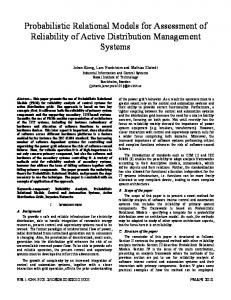
The RESCAL model was introduced in [17] and follows a similar dependency structure as the IHRM. The main difference is that the latent variables do not describe entity classes but are latent entity factors. The probability of a binary link is calculated as r r X
X GR P R(Ei , Ej ) = 1|A, GR ∝ k,l ai,k aj,l k=1 l=1

where r is the number of latent factors, A is the latent factor matrix and GR ∈ Rr×r is a full, asymmetric, relation-specific matrix. (A)i,k = ai,k ∈ R is the k-th factor of entity Ei and (A)j,l = aj,l ∈ R is the l-th factor of entity Ej . As in the IHRM, common children with observed values lead to interactions between the parent latent variables in the ground Bayesian network. This leads to the propagation of information in the network of latent variables and enables the learning of long-range dependencies. The relation-specific matrix GR encodes the factor interactions for a specific relation and its asymmetry permits the representation of directed relationships. The calculation of the latent factors is based on the factorization of a multirelational adjacency tensor where two modes represent the entities in the domain and the third mode represents the relation type (Figure 5). The relational

15

j-th entity i-th entity

A

GR AT

relation R

Figure 5: The figure illustrates the factorization of the multi-relational adjacency tensor used in the RESCAL model. In the multi-relational adjacency tensor on the left two modes represent the entities in the domain and the third mode represents the relation type. The i-th row of the matrix A contains the factors of the i-th entity. GR is a slice in the G-tensor and encodes the relation-type specific factor interactions. The factorization can be interpreted as a constrained Tucker decomposition. learning capabilities of the RESCAL model have been demonstrated on classification tasks and entity resolution tasks, i.e., the mapping of entities between knowledge bases. One of the great advantages of the RESCAL model is its scalability: RESCAL has been applied to the YAGO ontology [24] with several million entities and 40 relation types [18]! The YAGO ontology, closely related to DBpedia [2] and the Knowledge Graph [23], contains formalized knowledge from Wikipedia and other sources. RESCAL is part of a tradition on relation prediction using factorization of matrices and tensors. [30] describes a Gaussian process-based approach for predicting a single relation type, which has been generalized to a mutli-relational setting in [28]. Whereas RESCAL is calculated based on a constrained Tucker decomposition of the multi-relational adjacency tensor, the SUNS approach [27] is based on a Tucker1 decomposition.

10

Key Applications

Typical applications of relational models are in social networks analysis, bioinformatics, recommendation systems, language processing, medical decision support, knowledge bases, and Linked Open Data.

16

11

Future Directions

A wider application of relational models so far was hindered by their complexity and scalability issues. With a certain personal bias, we believe that the relational latent variable models (RESCAL, SUNS) point in a promising direction. Maybe an application with billions of internet users is still somewhat far in the future, an application with millions of patients is within reach.

References [1] Edoardo M. Airoldi, David M. Blei, Stephen E. Fienberg, and Eric P. Xing. Mixed membership stochastic blockmodels. Journal of Machine Learning Research, 9:1981–2014, 2008. [2] S¨ oren Auer, Christian Bizer, Georgi Kobilarov, Jens Lehmann, Richard Cyganiak, and Zachary G. Ives. Dbpedia: A nucleus for a web of open data. In ISWC/ASWC, pages 722–735, 2007. [3] Pedro Domingos and Matthew Richardson. Markov logic: A unifying framework for statistical relational learning. In Lise Getoor and Benjamin Taskar, editors, Introduction to Statistical Relational Learning, pages 339– 369. MIT Press, 2007. [4] Saso Dzeroski. Inductive logic programming in a nutshell. In Lise Getoor and Benjamin Taskar, editors, Introduction to Statistical Relational Learning, pages 57–92. MIT Press, 2007. [5] Nir Friedman, Lise Getoor, Daphne Koller, and Avi Pfeffer. Learning probabilistic relational models. In IJCAI, pages 1300–1309, 1999. [6] Lise Getoor, Nir Friedman, Daphne Koller, Avi Pferrer, and Benjamin Taskar. Probabilistic relational models. In Lise Getoor and Benjamin Taskar, editors, Introduction to Statistical Relational Learning, pages 129– 174. MIT Press, 2007. [7] David Heckerman, David Maxwell Chickering, Christopher Meek, Robert Rounthwaite, and Carl Myers Kadie. Dependency networks for inference, collaborative filtering, and data visualization. Journal of Machine Learning Research, 1:49–75, 2000. [8] David Heckerman, Christopher Meek, and Daphne Koller. Probabilistic entity-relationship models, prms, and plate models. In Lise Getoor and Benjamin Taskar, editors, Introduction to Statistical Relational Learning, pages 201–238. MIT Press, 2007. [9] Reimar Hofmann and Volker Tresp. Nonlinear markov networks for continuous variables. In NIPS, 1997.

17

[10] Manfred Jaeger. Relational bayesian networks. In UAI, pages 266–273, 1997. [11] Charles Kemp, Joshua B. Tenenbaum, Thomas L. Griffiths, Takeshi Yamada, and Naonori Ueda. Learning systems of concepts with an infinite relational model. In AAAI, pages 381–388, 2006. [12] Kristian Kersting and Luc De Raedt. Bayesian logic programs. CoRR, cs.AI/0111058, 2001. [13] Daphne Koller and Avi Pfeffer. Probabilistic frame-based systems. In AAAI/IAAI, pages 580–587, 1998. [14] Uta L¨ osch, Stephan Bloehdorn, and Achim Rettinger. Graph kernels for rdf data. In ESWC, pages 134–148, 2012. [15] Stephen Muggleton. Inductive logic programming. New Generation Comput., 8(4):295–318, 1991. [16] Jennifer Neville and David Jensen. Dependency networks for relational data. In ICDM, pages 170–177, 2004. [17] Maximilian Nickel, Volker Tresp, and Hans-Peter Kriegel. A three-way model for collective learning on multi-relational data. In ICML, pages 809– 816, 2011. [18] Maximilian Nickel, Volker Tresp, and Hans-Peter Kriegel. Factorizing yago: scalable machine learning for linked data. In WWW, pages 271–280, 2012. [19] J. Ross Quinlan. Learning logical definitions from relations. Machine Learning, 5:239–266, 1990. [20] Luc De Raedt and Luc Dehaspe. Clausal discovery. Machine Learning, 26(2-3):99–146, 1997. [21] Achim Rettinger, Matthias Nickles, and Volker Tresp. A statistical relational model for trust learning. In AAMAS (2), pages 763–770, 2008. [22] Matthew Richardson and Pedro Domingos. Markov logic networks. Machine Learning, 62(1-2):107–136, 2006. [23] Amit Singhal. Introducing the knowledge graph: things, not strings. Technical report, Ofcial Google Blog, May 2012. http://googleblog.blogspot.com/2012/05/introducing-knowledge-graphthings-not.html, 2012. [24] Fabian M. Suchanek, Gjergji Kasneci, and Gerhard Weikum. Yago: a core of semantic knowledge. In WWW, pages 697–706, 2007. [25] Dan Suciu, Dan Olteanu, Christopher R´e, and Christoph Koch. Probabilistic Databases. Synthesis Lectures on Data Management. Morgan & Claypool Publishers, 2011. 18

[26] Benjamin Taskar, Pieter Abbeel, and Daphne Koller. Discriminative probabilistic models for relational data. In UAI, pages 485–492, 2002. [27] Volker Tresp, Yi Huang, Markus Bundschus, and Achim Rettinger. Materializing and querying learned knowledge. In First ESWC Workshop on Inductive Reasoning and Machine Learning on the Semantic Web (IRMLeS 2009), 2009. [28] Zhao Xu, Kristian Kersting, and Volker Tresp. Multi-relational learning with gaussian processes. In IJCAI, pages 1309–1314, 2009. [29] Zhao Xu, Volker Tresp, Kai Yu, and Hans-Peter Kriegel. Infinite hidden relational models. In UAI, 2006. [30] Kai Yu, Wei Chu, Shipeng Yu, Volker Tresp, and Zhao Xu. Stochastic relational models for discriminative link prediction. In NIPS, pages 1553– 1560, 2006.

19