Social Network Mining with Nonparametric Relational Models Zhao Xu1 , Volker Tresp2 , Achim Rettinger3 , and Kristian Kersting1 1
Fraunhofer IAIS, Germany
[email protected] Siemens Corporate Technology, Germany
[email protected] Technical University of Munich, Germany
[email protected]
2 3
Abstract. Statistical relational learning (SRL) provides effective techniques to analyze social network data with rich collections of objects and complex networks. Infinite hidden relational models (IHRMs) introduce nonparametric mixture models into relational learning and have been successful in many relational applications. In this paper we explore the modeling and analysis of complex social networks with IHRMs for community detection, link prediction and product recommendation. In an IHRM-based social network model, each edge is associated with a random variable and the probabilistic dependencies between these random variables are specified by the model, based on the relational structure. The hidden variables, one for each object, are able to transport information such that non-local probabilistic dependencies can be obtained. The model can be used to predict entity attributes, to predict relationships between entities and it performs an interpretable cluster analysis. We demonstrate the performance of IHRMs with three social network applications. We perform community analysis on the Sampson’s monastery data and perform link analysis on the Bernard & Killworth data. Finally we apply IHRMs to the MovieLens data for prediction of user preference on movies and for an analysis of user clusters and movie clusters. Key words: Statistical Relational Learning, Social Network Analysis, Nonparametric Mixture Models, Dirichlet Process, Variational Inference
1
Introduction
Social network mining has gained in importance due to the growing availability of data on novel social networks, e.g. citation networks (DBLP, Citeseer), SNS websites (Facebook), and social media websites (Last.fm). Social networks usually consist of rich collections of objects, which are linked into complex networks. Generally, social network data can be graphically represented as a sociogram as illustrated in Fig. 1 (left). In this simple social network, there are persons, person profiles (e.g., gender), and these persons are linked together via friendships. Some interesting applications in social network mining include community discovery, relationship prediction, social recommendation, etc. Statistical relational learning (SRL) [8, 17, 11] is an emerging area of machine learning research, which attempts to combine expressive knowledge representation formalisms with statistical approaches to perform probabilistic inference
2
Zhao Xu, Volker Tresp, Achim Rettinger, and Kristian Kersting
and learning on relational networks. Fig. 1 (right) shows a simple SRL model for the above sociogram example. For each potential edge, a random variable (RV) is introduced that describes the state of the edge. For example, there is a RV associated with the edge between the person 1 and the person 2. The binary variable is YES if the two persons are friends and No otherwise. The edge between an object (e.g., person 1) and object property (e.g., Male) is also associated with a RV, whose value describes the person’s profile. In the running example, all variables are binary. To infer the quantities of interest, e.g., whether the person 1 and the person 2 are friends, we need to learn the probabilistic dependencies between the random variables. Here we assume that friendship is conditioned on the profiles (gender) of the involved persons, shown as Fig. 1 (right). The directed arcs, for example, the ones between G1 and R1,2 and between G2 and R1,2 specify that the probability that person 1 and the person 2 are friends depends on their respective profiles. Given the probabilistic model, we can learn the parameters and predict the relationships of interest.
Fig. 1. Left: A simple sociogram. Right: A probabilistic model for the sociogram. Each edge is associated with a random variable that determines the state of the edge. The directed arcs indicate direct probabilistic dependencies.
In the simple relational model of social network, the friendship is locally predicted by the profiles of the involved objects: whether a person is a friend of another person is only dependent on the profiles of the two persons. Given that the parameters are fixed, and given the parent attributes, all friendships are independent of each other such that correlations between friendships, i.e., the collaborative effect, cannot be taken into account. To solve this limitation, structural learning might be involved to obtain non-local dependencies but structural learning in complex relational networks is considered a hard problem [9]. Non-local dependencies can also be achieved by introducing for each person a hidden variable as proposed in [24]. The state of the hidden variable represents unknown attributes of the person, e.g. the particular habit of making friends with certain persons. The hidden variable of a person is now the only parent of its profiles and is one of the parents of the friendships in which the person potentially participates. Since the hidden variables are of central importance,
Social Network Mining with Nonparametric Relational Models
3
this model is referred to as the hidden relational model (HRM). In relational domains, different classes of objects generally require a class-specific complexity in the hidden representation. Thus, it is sensible to work with a nonparametric method, Dirichlet process (DP) mixture model, in which each object class can optimize its own representational complexity in a self-organized way. Conceptionally, the number of states in the hidden variables in the HRM model becomes infinite. In practice, the DP mixture sampling process only occupies a finite number of components. The combination of the hidden relational model and the DP mixture model is the infinite hidden relational model (IHRM) [24]. The IHRM model has been first presented in [24]. This paper is an extended version of [25] and we explore social network modeling and analysis with IHRM for community detection, link prediction, and product recommendation. We present two inference methods for efficient inference: one is the blocked Gibbs sampling with truncated stick-breaking (TSB) construction, the other is the mean-field approximation with TSB. We perform empirical analysis on three social network datasets: the Sampson’s monastery data, the Bernard & Killworth data, and the MovieLens data. The paper is organized as follows. In the next section, we perform analysis of modeling complex social network data with IHRMs. In Sec. 3 we describe a Gibbs sampling method and a mean-field approximation for inference in the IHRM model. Sec. 4 gives the experimental analysis on social network data. We review some related work in Sec. 5. Before concluding, an extension to IHRMs is discussed in Sec. 6.
2
Model Description
Based on the analysis in Sec. 1, we will give a detailed description of the IHRM model for social network data. In this section, we first introduce the finite hidden relational model (HRM), and then extend it to an infinite version (IHRM). In addition, we provide a generative model describing how to generate data from an IHRM model. 2.1
Hidden Relational Model
A hidden relational model (HRM) for a simple sociogram is shown in Fig. 2. The basic innovation of the HRM model is introducing for each object (here: person) a hidden variable, denoted as Z in the figure. They can be thought of as unknown attributes of persons. We then assume that attributes of a person only depend on the hidden variable of the person, and a relationship only depends on the hidden variables of the persons involved in the relationship. It implies that if hidden variables were known, both person attributes and relationships can be well predicted. Given the HRM model shown in Fig. 2, information can propagate via interconnected hidden variables. Let us predict whether the person 2 will be a friend of the person 3, i.e. predict the relationship R2,3 . The probability is computed on the evidence about: (1) the attributes of the immediately related persons,
4
Zhao Xu, Volker Tresp, Achim Rettinger, and Kristian Kersting
Fig. 2. A hidden relational model (HRM) for a simple sociogram.
i.e. G2 and G3 , (2) the known relationships associated with the persons of interest, i.e. the friendships R2,1 and R2,4 about the person 2, and the friendships R1,3 and R3,4 about the person 3, (3) high-order information transferred via hidden variables, e.g. the information about G1 and G4 propagated via Z1 and Z4 . If the attributes of persons are informative, those will determine the hidden states of the persons, therefore dominate the computation of predictive probability of relationship R2,3 . Conversely, if the attributes of persons are weak, then hidden state of a person might be determined by his relationships to other persons and the hidden states of those persons. By introducing hidden variables, information can globally distribute in the ground network defined by the relational structure. This reduces the need for extensive structural learning, which is particularly difficult in relational models due to the huge number of potential parents. Note that a similar propagation of information can be observed in hidden Markov models used in speech recognition or in the hidden Markov random fields used in image analysis [26]. In fact, the HRM can be viewed as a directed generalization of both for relational data. Additionally, the HRM provides a cluster analysis of relational data. The state of the hidden variable of an object corresponds to its cluster assignment. This can be regarded as a generalization of co-clustering model [13]. The HRM can be applied to domains with multiple classes of objects and multiple classes of relationships. Furthermore, relationships can be of arbitrary order, i.e. the HRM is not constraint to only binary and unary relationships[24]. Also note that the sociogram is quite related to the resource description framework (RDF) graph used as the basic data model in the semantic web [3] and the entity relationship graph from database design. We now complete the model by introducing the variables and parameters in Fig. 2. There is a hidden variable Zi for each person. The state of Zi specifies the cluster of the person i. Let K denote the number of clusters. Z follows Pa multinomial distribution with parameter vector π = (π1 , . . . , πK ) (πk > 0, k πk = 1), which specifies the probability of a person belonging to a cluster, i.e. P (Zi = k) = πk . π is sometimes referred to as mixing weights. It is drawn from a conjugated Dirichlet prior with hyperparameters α0 .
Social Network Mining with Nonparametric Relational Models
5
All person attributes are assumed to be discrete and multinomial variables (resp., binary and Bernoulli). Thus a particular person attribute Gi is a sample drawn from a multinomial (resp., Bernoulli) distribution with parameters θk , where k denotes the cluster assignment of the person. θk is sometimes referred to as mixture component, which is associated with the cluster k. For all persons, there are totally K mixture components Θ = (θ1 , . . . , θK ). Each person in the cluster k inherits P the mixture component, thus we have: P (Gi = s|Zi = k, Θ) = θk,s (θk,s > 0, s θk,s = 1). These mixture components are independently drawn from a prior G0 . For computational efficiency, we assume that G0 is a conjugated Dirichlet prior with hyperparameters β. We now consider the variables and parameters concerning the relationships (FriendOf). The relationship R is assumed to be discrete with two states. A particular relationship Ri,j between two persons (i and j) is a sample drawn from a binomial distribution with a parameter φk,` , where k and ` denote cluster assignments of the person i and the person j, respectively. There are totally K × K parameters φk,` , and each φk,` is independently drawn from the prior Gr0 . For computational efficiency, we assume that Gr0 is a conjugated Beta distribution with hyperparameters β r . From a mixture model point of view, the most interesting term in the HRM model is φk,` , which can be interpreted as a correlation mixture component. If a person i is assigned to a cluster k, i.e. Zi = k, then the person inherits not only θk , but also φk,` , ` = {1, . . . , K}. 2.2
Infinite Hidden Relational Model
Since hidden variables play a key role in the HRM model, we would expect that the HRM model might require a flexible number of states for the hidden variables. Consider again the sociogram example. With little information about past friendships, all persons might look the same; with more information available, one might discover certain clusters in persons (different habits of making friends); but with an increasing number of known friendships, clusters might show increasingly detailed structure ultimately indicating that everyone is an individual. It thus makes sense to permit an arbitrary number of clusters by using a Dirichlet process mixture model. This permits the model to decide itself about the optimal number of clusters and to adopt the optimal number with increasing data. For our discussion it suffices to say that we obtain an infinite HRM by simply letting the number of clusters approach infinity, K → ∞. Although from a theoretical point of view there are indeed an infinite number of components, a sampling procedure would only occupy a finite number of components. The graphical representations of the IHRM and HRM models are identical, shown as Fig. 2. However, the definitions of variables and parameters are different. For example, hidden variables Z of persons have infinite states, and thus parameter vector π is infinite-dimensional. The parameter is not generated from a Dirichlet prior, but from a stick breaking construction Stick(·|α0 ) with a hyperparameter α0 (more details in the next section). Note that α0 is a positive real-valued scalar and is referred to as concentration parameter in DP mixture
6
Zhao Xu, Volker Tresp, Achim Rettinger, and Kristian Kersting
modeling. It determines the tendency of the model to either use a large number or a small number of states in the hidden variables [2]. If α0 is chosen to be small, only few clusters are generated. If α0 is chosen to be large, the coupling is loose and more clusters are formed. Since there are an infinite number of clusters, there are an infinite number of mixture components θk , each of which is still independently drawn from G0 . G0 is referred to as base distribution in DP mixture modeling. 2.3
Generative Model
Now we describe the generative model for the IHRM model. There are mainly two methods to generate samples from a Dirichlet Process (DP) mixture model, i.e. the Chinese restaurant process (CRP) [2] and the stick breaking construction (SBC) [22]. We will discuss how SBC can be applied to the IHRM model (see [24] for CRP-based generative model). Notations is summarized in Table 1. Table 1. Notation used in this paper. Symbol C B Nc αc0 eci Aci θkc Gc0 βc b Ri,j φbk,` Gb0 βb
Description number of object classes number of relationship classes number of objects in a class c concentration parameter of an object class c an object indexed by i in a class c an attribute of an object eci mixture component indexed by a hidden state k in an object class c base distribution of an object class c parameters of a base distribution Gc0 relationship of class b between objects i, j correlation mixture component indexed by hidden states k for ci and ` for cj , where ci and cj are object classes involved in a relationship class b base distribution of a relationship class b parameters of a base distribution Gb0
The stick breaking construction (SBC) [22] is a representation of DPs, by which we can explicitly sample random distributions of attribute parameters and relationship parameters. In the following we describe the generative model of IHRM in terms of SBC. 1. For each object class c, (a) Draw mixing weights π c ∼ Stick(·|α0c ), defined as iid
Vkc ∼ Beta(1, αc0 );
π1c = V1c , πkc = Vkc
k−1 Y
(1 − Vkc0 ), k > 1.
k0 =1
(1)
Social Network Mining with Nonparametric Relational Models
7
(b) Draw i.i.d. mixture components θkc ∼ Gc0 , k = 1, 2, . . . 2. For each relationship class b between two object classes ci and cj , draw φbk,` ∼ Gb0 i.i.d. with component indices k for ci and ` for cj . 3. For each object eci in a class c, (a) Draw cluster assignment Zic ∼ Mult(·|π c ); (b) Draw object attributes Aci ∼ P (·|θc , Zic ). c c b ∼ P (·|φb , Zici , Zj j ). 4. For eci i and ejj with a relationship of class b, draw Ri,j The basic property of SBC is that: the distributions of the parameters (θkc and φbk,` ) are sampled, e.g., the distribution of θkc can be represented as Gc = P∞ c c c c k=1 πk δθk , where δθk is a distribution with a point mass on θk . In terms of this property, SBC can sample objects independently; thus it might be efficient when a large domain is involved.
3
Inference
The key inferential problem in the IHRM model is computing posterior of unobservable variables given the data, i.e. P ({π c , Θc , Z c }c , {Φb }b |D, {α0c , Gc0 }c , {Gb0 }b ). Unfortunately, the computation of the joint posterior is analytically intractable, thus we consider approximate inference methods to solve the problem. 3.1
Inference with Gibbs Sampling
Markov chain Monte Carlo (MCMC) sampling has been used to approximate posterior distribution with a DP mixture prior. In this section, we describe the efficient blocked Gibbs sampling (GS) with truncated stick breaking representation [14] for the IHRM model. The advantage is that given the posterior distributions, we can independently sample hidden variables in a block, which highly accelerates the computation. The Markov chain is thus defined not only on hidden variables, but also on parameters. Truncated stick breaking construction (TSB) fixes a value K c for each class of objects by letting VKc c = 1. That means the mixing weights πkc are equal to 0 for k > K c (refer to Equ. 1). The number of the clusters is thus reduced to K c . Note, that K c is an additional parameter in the inference method. At each iteration, we first update the hidden variables conditioned on the parameters sampled in the last iteration, and then update the parameters conditioned on the hidden variables. In detail: 1. For each class of objects, c(t+1) (a) Update each hidden variable Zi with probability proportional to: c(t)
c(t+1)
πk P (Aci |Zi
= k, Θc(t) )
YY b0
0
c(t+1)
b 0 |Zi P (Ri,j
c 0 (t)
= k, Zj 0j
0
, Φb (t) ), (2)
j0
0
b where Aci and Ri,j 0 denotes the known attributes and relationships about c 0 (t)
i. cj 0 denotes the class of the object j 0 , Zj 0j denotes hidden variable of j 0 at the last iteration t. Intuitively, the equation represents to what extent the cluster k agrees with the data Dic about the object i.
8
Zhao Xu, Volker Tresp, Achim Rettinger, and Kristian Kersting
(b) Update π c(t+1) as follows: c(t+1) c(t+1) c(t+1) from Beta(λk,1 , λk,2 ) for k = {1, . . . , K c − 1} i. Sample vk c
c(t+1)
λk,1
=1+
N X
c
c(t+1)
δk (Zi
c(t+1)
), λk,2
= α0c +
c(t+1)
δk0 (Zi
), (3)
k0 =k+1 i=1
i=1
c(t+1)
c
K N X X
c(t+1)
c(t+1)
and set vK c = 1. δk (Zi ) equals to 1 if Zi = k and 0 otherwise. c(t+1) c(t+1) Qk−1 c(t+1) ii. Compute π c(t+1) as: πk = vk ) for k > 1 k0 =1 (1 − vk0 c(t+1) c(t+1) and π1 = v1 . c(t+1) b(t+1) 2. Update θk ∼ P (·|Ac , Z c(t+1) , Gc0 ) and φk,` ∼ P (·|Rb , Z (t+1) , Gb0 ). The parameters are drawn from their posterior distributions conditioned on the sampled hidden states. Again, since we assume conjugated priors as the base distributions (Gc0 and Gb0 ), the simulation is tractable. After convergence, we collect the last W samples to make predictions for the relationships of interest. Note that in blocked Gibbs sampling, the MCMC sequence is defined by hidden variables and parameters, including Z c(t) , π c(t) , b Θc(t) , and Φb(t) . The predictive distribution of a relationship Rnew,j between a cj c new object enew and a known object ej is approximated as b b B P (Rnew,j |D, {α0c , Gc0 }C c=1 , {G0 }b=1 )
≈
W +w 1 X b b(t) B P (Rnew,j |D, {Z c(t) , π c(t) , Θ c(t) }C }b=1 ) c=1 , {Φ W t=w+1 c
W +w K YY 1 X X b(t) c(t) c(t) b0 (t) b b0 0 |φ ∝ P (Rnew,j |φk,` ) πk P (Acnew |θk ) P (Rnew,j k,`0 ), W t=w+1 0 0 k=1
b
j
where ` and `0 denote the cluster assignments of the objects j and j 0 , respectively. The equation is quite intuitive. The prediction is a weighted sum of predictions b(t) b P (Rnew,j |φk,` ) over all clusters. The weight of each cluster is the product of the last three terms, which represents to what extent this cluster agrees with the known data (attributes and relationships) about the new object. Since the blocked method also samples parameters, the computation is straightforward. 3.2
Inference with Variational Approximation
The IHRM model has multiple DPs which interact through relationships, thus blocked Gibbs sampling is still slow due to the slow exchange of information between DPs. To solve the problem, we outline an alternative solution by variational inference method. The main strategy is to convert a probabilistic inference problem into an optimization problem, and then to solve the problem with the known optimization techniques. In particular, the method assumes a distribution q, referred to as a variational distribution, to approximate the true posterior P as close as possible. The difference between the variational distribution q and the true posterior P can be measured via Kullback-Leibler (KL) divergence. Let
Social Network Mining with Nonparametric Relational Models
9
ξ denote a set of unknown quantities, and D denote the known data. The KL divergence between q(ξ) and P (ξ|D) is defined as: KL(q(ξ)||P (ξ|D)) =
X
q(ξ) log q(ξ) −
X
ξ
q(ξ) log P (ξ|D).
(4)
ξ
The smaller the divergence, the better is the fit between the true and the approximate distributions. The probabilistic inference problem (i.e. computing the posterior) now becomes: to minimize the KL divergence with respect to the variational distribution. In practice, the minimization of the KL divergence is formulated as the maximization of the lower bound of the log-likelihood: log P (D) ≥
X
q(ξ) log P (D, ξ) −
X
ξ
q(ξ) log q(ξ).
(5)
ξ
A mean-field method was explored in [6] to approximate the posterior of unobservable quantities in a DP mixture model. The main challenge of using mean-field inference for the IHRM model is that there are multiple DP mixture models coupled together with relationships and correlation mixture components. In the IHRM model, unobservable quantities include Z c , π c , Θc and Φb . Since mixing weights π c are computed on V c (see Equ. 1), we can replace π c with V c in the set of unobservable quantities. To approximate the posterior P ({V c , Θc , Z c }c , {Φb }b |D, {α0c , Gc0 }c , {Gb0 }b ), we define a variational distribution b B q({Z c , V c , Θc }C c=1 , {Φ }b=1 ) as: "
c
C Y N Y c
#
c
q(Zic |ηic )
i
K Y
q(Vkc |λck )q(θkc |τkc )
k
b
k
c
c
B K Y Yi K Yj
q(φbk,` |ρbk,` ) ,
(6)
`
where ci and cj denote the object classes involved in the relationship class b. k and ` denote the cluster indexes for ci and cj . Variational parameters include {ηic , λck , τkc , ρbk,` }. q(Zic |ηic ) is a multinomial distribution with parameters ηic . Note, that there is one ηic for each object eci . q(Vkc |λck ) is a Beta distribution. q(θkc |τkc ) and q(φbk,` |ρbk,` ) are respectively with the same forms as Gc0 and Gb0 . We substitute Equ. 6 into Equ. 5 and optimize the lower bound with a coordinate ascent algorithm, which generates the following equations to iteratively update the variational parameters until convergence: c
λck,1
=1+
N X
c
c ηi,k ,
λck,2
=
αc0
+
c
N K X X
c
c τk,1 = β1c +
N X
X
Ã
c τk,2 = β2c +
c
ci b j ηj,` T(Ri,j ), ηi,k
(8)
X
c
ci j ηj,` , ηi,k
(9)
i,j k−1 X
Eq [log(1 − Vkc0 )] + Eq [log P (Aci |θkc )]
k0 =1
j
c ηi,k ,
ρbk,`,2 = β2b +
i,j
XXX b0
N X i=1
c ηi,k ∝ exp Eq [log Vkc ] +
+
(7)
c
c ηi,k T(Aci ),
i=1
ρbk,`,1 = β1b +
c 0, ηi,k
i=1 k0 =k+1
i=1
`
c
! 0
0
b b j ηj,` Eq [log P (Ri,j |φk,` )] ,
(10)
10
Zhao Xu, Volker Tresp, Achim Rettinger, and Kristian Kersting
where λck denotes parameters of Beta distribution q(Vkc |λck ), λck is a two-dimensional vector λck = (λck,1 , λck,2 ). τkc denotes parameters of the exponential family distric bution q(θkc |τkc ). We decompose τkc such that τk,1 contains the first dim(θkc ) comc c ponents and τk,2 is a scalar. Similarly, β1 contain the first dim(θkc ) components and β2c is a scalar. ρbk,`,1 , ρbk,`,2 , β1b and β2b are defined equivalently. T(Aci ) and b T(Ri,j ) denote the sufficient statistics of the exponential family distributions b P (Aci |θkc ) and P (Ri,j |φbk,` ), respectively. It is clear that Equ. 7 and Equ. 8 correspond to the updates for variational parameters of object class c, and they follow equations in [6]. Equ. 9 represents the updates of variational parameters for relationships, which is computed on the involved objects. The most interesting updates are Equ. 10, where the posteriors of object cluster-assignments are coupled together. These essentially connect the c include a DPs together. Intuitively, in Equ. 10 the posterior updates for ηi,k prior term (first two expectations), the likelihood term about object attributes (third expectation), and the likelihood terms about relationships (last term). To calculate the last term we need to sum over all the relationships of the object cj eci weighted by ηj,` that is variational expectation about cluster-assignment of the other object involved in the relationship. Once the procedure reaches stationarity, we obtain the optimized variational parameters, by which we can approximate the predictive distribution b b B b |D, {α0c , Gc0 }C P (Rnew,j c=1 , {G0 }b=1 ) of the relationship Rnew,j between a new cj c b object enew and a known object ej with q(Rnew,j |D, λ, η, τ, ρ) proportional to: c
c
K K X Xj k
c
c
b c q(Rnew,j |ρbk,` )q(Zj j = `|ηj j )q(Znew = k|λc )
`
× q(Acnew |τkc )
YYX b0
j0
c 0
c 0
0
0
b b 0 |ρk,`0 ). q(Zj 0j = `0 |ηj 0j )q(Rnew,j
(11)
`0
b |ρbk,` ) over all clusters. The prediction is a weighted sum of predictions q(Rnew,j The weight consists of two parts. One is to what extent the cluster ` agrees with c the object ejj (i.e. the 2nd term), the other is to what extent the cluster k agrees with the new object (i.e. the product of the last 3 terms). The computations c about the two parts are different. The reason is that ejj is a known object, we c have optimized variational parameters ηj j about its cluster assignment.
4 4.1
Experimental Analysis Monastery Data
The first experiment is performed on the Sampson’s monastery dataset [19] for community discovery. Sampson surveyed social relationships between 18 monks in an isolated American monastery. The relationships between monks included esteem/disesteem, like/dislike, positive influence/negative influence, praise and blame. Breiger et al. [7] summarized these relationships and yielded a single
Social Network Mining with Nonparametric Relational Models
11
2 4 6 8 10 12 14 16 18 2
4
6
8
10
12
14
16
18
Fig. 3. Left: The matrix displaying interactions between Monks. Middle: A sociogram for three monks. Right: The IHRM model for the monastery sociogram.
relationship matrix, which reflected interactions between monks, as shown in Fig. 3 (left). After observing the monks in the monastery for several months, Sampson provided a description of the factions among the monks: the loyal opposition (Peter, Bonaventure, Berthold, Ambrose and Louis), the young turks (John Bosco, Gregory, Mark, Winfrid, Hugh, Boniface and Albert) and the outcasts (Basil, Elias and Simplicius). The other three monks (Victor, Ramuald and Amand) wavered between the loyal opposition and the young turks, and were identified as the fourth group, the waverers. Sampson’s observations were confirmed by the event that the young turks group resigned after the leaders of the group were expelled over religious differences. The task of the experiment is to cluster the monks. Fig. 3 (middle) shows a sociogram with 3 monks. The IHRM model for the monastery network is illustrated as Fig. 3 (right). There is one hidden variable for each monk. The relationships between monks are conditioned on the hidden variables of the involved monks. The mean field method is used for inference. We initially assume that each monk is in his own cluster. After convergence, the cluster number is optimized as 4, which is exactly the same as the number of the groups that Sampson identified. The clustering result is shown as Table 2. It is quite close to the real groups. Cluster 1 corresponds to the loyal opposition. Cluster 2 is the young turks, and cluster 3 is the outcasts. The waverers are split. Amand is assigned to cluster 4, Victor and Ramuald are assigned to the loyal opposition. Actually, previous research analysis has questioned the distinction of the waverers, e.g., [7, 12] clustered Victor and Ramuald into the loyal opposition, which coincides with the result of the IHRM model. Table 2. Clustering result of the IHRM model on Sampson’s monastery data. Cluster 1 2 3 4
Members Peter, Bonaventure, Berthold, Ambrose, Louis, Victor, Ramuald John, Gregory, Mark, Winfrid, Hugh, Boniface, Albert Basil, Elias, Simplicius Amand
12
Zhao Xu, Volker Tresp, Achim Rettinger, and Kristian Kersting Table 3. Link prediction on the Bernard & Killworth data with the IHRM.
50% IHRM Pearson BKFRAT 66.50 61.82 BKOFF 66.21 57.32 BKTEC 65.47 58.85
4.2
Prediction Accuracy (%) 60% 70% IHRM Pearson IHRM Pearson 67.63 64.56 68.26 66.91 67.89 59.45 69.20 60.58 66.79 62.04 68.31 63.61
80% IHRM Pearson 68.69 67.41 69.82 61.54 69.58 64.46
Bernard & Killworth Data
Fig. 4. Left: Interaction matrix on the BKOFF data. Right: The predicted one, which is quite similar with the real situation.
In the second experiment, we perform link analysis with IHRM on the Bernard & Killworth data [5]. Bernard and Killworth collected several data sets on human interactions in bounded groups. In each study they obtained measures of social interactions among all actors, and ranking data based on the subjects’ memory of those interactions. Our experiments are based on three datasets. The BKFRAT data is about interactions among students living in a fraternity at a West Virginia college. All subjects had been residents in the fraternity from three months to three years. The data consists of rankings made by the subjects of how frequently they interacted with other subjects in the observation week. The BKOFF data concern interactions in a small business office. Observations were made as the observer patrolled a fixed route through the office every fifteen minutes during two four-day periods. The data contains rankings of interaction frequency as recalled by employees over the two-week period. The BKTEC data is about interactions in a technical research group at a West Virginia university. It contains the personal rankings of the remembered frequency of interactions. In the experiments, we randomly select 50% (60%, 70%, 80%) interactions as known and predict the left ones. The experiments are repeated 20 times for each
Social Network Mining with Nonparametric Relational Models
13
setting. The average prediction accuracy is reported in Table 3. We compare our model with the Pearson collaborative filtering method. It shows that the IHRM model provides better performance on all the three datasets. Fig. 4 illustrates the link prediction results on the BKOFF dataset with 70% known links. The predicted interaction matrix is quite similar with the real one. 4.3
MovieLens Data
Fig. 5. Top: A sociogram for movie recommendation system, illustrated with 2 users and 3 movies. For readability, only two attributes (user’s occupation and movie’s genre) show in the figure. Bottom: The IHRM model for the sociogram.
We also evaluate the IHRM model on the MovieLens data [21]. There are in total 943 users and 1680 movies, and we obtain 702 users and 603 movies after removing low-frequent ones. Each user has about 112 ratings on average. The model is shown in Fig. 5. There are two classes of objects (users and movies) and one class of relationships (Like). The task is to predict preferences of users. The users have attributes Age, Gender, Occupation, and the movies have attributes Published-year, Genres and so on. The relationships have two states, where R = 1 indicates that the user likes the movie and 0 otherwise. The user ratings in MovieLens are originally based on a five-star scale, so we transfer each rating to binary value with R = 1 if the rating is higher than the user’s average rating, vice versa. The performance of the IHRM model is analyzed from 2 points: prediction accuracy and clustering effect. To evaluate the prediction performance, we perform 4 sets of experiments which respectively select 5, 10, 15 and 20 ratings for each test user as the known ratings, and predict the remaining ratings. These experiments are referred to as given5, given10, given15 and given20 in the following. For testing the relationship is predicted to exist (i.e., R = 1) if the predictive probability is larger than a threshold ε = 0.5.
14
Zhao Xu, Volker Tresp, Achim Rettinger, and Kristian Kersting
Fig. 6. Left: The traces of the number of user clusters for the runs of two Gibbs samplers. Middle: The trace of the change of the variational parameter η u for mean field method. Right: The sizes of the largest user clusters of the three inference methods.
We implement the following three inference methods: Chinese restaurant process Gibbs sampling (CRPGS), truncated stick-breaking Gibbs sampling (TSBGS), and the corresponding mean field method TSBMF. The truncation parameters Ks for TSBGS and TSBMF are initially set to be the number of entities. For TSBMF we consider α0 = {5, 10, 100, 1000}, and obtain the best prediction when α0 = 100. For CRPGS and TSBGS α0 is 100. For the variational inference, the change of variational parameters between two iterations is monitored to determine the convergence. For the Gibbs samplers, the convergence was analyzed by three measures: Geweke statistic on likelihood, Geweke statistic on the number of components for each class of objects, and autocorrelation. Fig. 6 (left) shows the trace of the number of user clusters in the 2 Gibbs samplers. Fig. 6 (middle) illustrates the change of variational parameters η u in the variational inference. For CRPGS, the first w = 50 iterations (6942 s) are discarded as burn-in period, and the last W = 1400 iterations are collected to approximate the predictive distributions. For TSBGS, we have w = 300 (5078 s) and W = 1700. Although the number of iterations for the burn-in period is much less in the CRPGS if compared to the blocked Gibbs sampler, each iteration is approximately a factor 5 slower. The reason is that CRPGS samples the hidden variables one by one, which causes two additional time costs. First, the expectations of attribute parameters and relational parameters have to be updated when sampling each user/movie. Second, the posterior of hidden variables have to be computed one by one, thus we can not use fast matrix multiplication techniques to accelerate the computation. Therefore if we include the time, which is required to collect a sufficient number of samples for inference, the CRPGS is slower by a factor of 5 (the row Time(s) in Table 4 ) than the blocked sampler. The mean field method is again by a factor around 10 faster than the blocked Gibbs sampler and thus almost two orders of magnitude faster than the CRPGS. The prediction results are shown in Table 4. All IHRM inference methods under consideration achieve comparably good performance; the best results are achieved by the Gibbs samplers. To verify the performance of the IHRM, we also implement Pearson-coefficient collaborative filtering (CF) method [18] and a SVD-based CF method [20]. It is clear that the IHRM outperforms the traditional CF methods, especially when there are few known ratings for the test
Social Network Mining with Nonparametric Relational Models
15
Table 4. Performance of the IHRM model on MovieLens data.
Given5 Given10 Given15 Given20 Time(s) Time/iter. #C.u #C.m
CRPGS 65.13 65.71 66.73 68.53 164993 109 47 77
TSBGS 65.51 66.35 67.82 68.27 33770 17 59 44
TSBMF 65.26 65.83 66.54 67.63 2892 19 9 6
Pearson 57.81 60.04 61.25 62.41 -
SVD 63.72 63.97 64.49 65.13 -
users. The main advantage of the IHRM is that it can exploit attribute information. If the information is removed, the performance of the IHRM becomes close to the performance of the SVD approach. For example, after ignoring all attribute information, the TSBMF generates the predictive results: 64.55% for Given5, 65.45% for Given10, 65.90% for Given15, and 66.79% for Given20. The IHRM provides cluster assignments for all objects involved, in our case for the users and the movies. The rows #C.u and #C.m in Table 4 denote the number of clusters for users and movies, respectively. The Gibbs samplers converge to 46-60 clusters for the users and 44-78 clusters for the movies. The mean field solution have a tendency to converge to a smaller number of clusters, depending on the value of α0 . Further analysis shows that the clustering results of the methods are actually similar. First, the sizes of most clusters generated by the Gibbs samplers are very small, e.g., there are 72% (75.47%) user clusters with less than 5 members in CRPGS (TSBGS). Fig. 6 (right) shows the sizes of the 20 largest user clusters of the 3 methods. Intuitively, the Gibbs samplers tend to assign the outliers to new clusters. Second, we compute the rand index (0-1) of the clustering results of the methods, the values are 0.8071 between CRPGS and TSBMF, 0.8221 between TSBGS and TSBMF, which demonstrates the similarity of the clustering results. Fig. 7 gives the movies with highest posterior probability in the 4 largest clusters generated from TSBMF. In cluster 1 most movies are very new and popular (the data set was collected from September 1997 through April 1998). Also they tend to be action and thriller movies. Cluster 2 includes many old movies, or movies produced by the non-USA countries. They tend to be drama movies. Cluster 3 contains many comedies. In cluster 4 most movies include relatively serious themes. Overall we were quite surprised by the good interpretability of the clusters. Fig. 8 (top) shows the relative frequency coefficient (RFC) of the attribute Genre in these movie clusters. RFC of a genre s in a cluster k is calculated as (fk,s − fs )/σs , where fk,s is the frequency of the genre s in the movie cluster k, fs is mean frequency, and σs is standard deviation of frequency. The labels for each cluster specify the dominant genres in the cluster. For example, action and thriller are the two most frequent genres in cluster 1. In
16
Zhao Xu, Volker Tresp, Achim Rettinger, and Kristian Kersting
Fig. 7. The major movie clusters generated by TSBMF on MovieLens data.
general, each cluster involves several genres. It is clear that the movie clusters are related to, but not just based on, the movie attribute Genre. The clustering effect depends on both movie attributes and user ratings. Fig. 8 (bottom) shows RFC of the attribute Occupation in user clusters. Equivalently, the labels for each user cluster specify the dominant occupations in the cluster. Note that in the experiments we predicted a relationship attribute R indicating the rating of a user for a movie. The underlying assumption is that in principle anybody can rate any movie, no matter whether that person has watched the movie or not. If the latter is important, we could introduce an additional attribute Exist to specify if a user actually watched the movie. The relationship R would then only be included in the probabilistic model if the movie was actually watched by a user.
5
Related Work
The work on infinite relational model (IRM) [15] is similar to the IHRM, and has been developed independently. One difference is that the IHRM can specify any reasonable probability distribution for an attribute given its parent, whereas the IRM would model an attribute as a unary predicate, i.e. would need to transform the conditional distribution into a logical binary representation. Aukia et al. also developed a DP mixture model for large networks [4]. The model associates an infinite-dimensional hidden variable for each link (relationship), and the objects involved in the link are drawn from a multinomial distribution conditioned on the hidden variable of the link. The model is applied to the community web data with promising experimental results. The latent mixed-membership model [1] can be viewed as a generalization of LDA model on relational data. Although
Social Network Mining with Nonparametric Relational Models
17
Fig. 8. Top: The relative frequency coefficient of the attribute Genre in different movie clusters, Bottom: that of the attribute Occupation in different user clusters.
it is not nonparametric, the model exploits hidden variables to avoid the extensive structure learning and provides a principled way to model the relational networks. The model associates each object with a membership probability-like vector. For each relationship, cluster assignments of the involved objects are generated with respect to their membership vectors, and then relationship is drawn conditioned on the cluster assignments. There are some other important SRL research works for complex relational networks. The probabilistic relational model (PRM) with class hierarchies [10] specializes distinct probabilistic dependency for each subclass, and thus obtains refined probabilistic models for relational data. A group-topic model is proposed in [23]. It jointly discovers latent groups in a network as well as latent topics of events between objects. The latent group model in [16] introduces two latent variables ci and gi for an object, and ci is conditioned on gi . The object attributes depends on ci and relations depend on gi of the involved objects. The limitation is that only relations between members in the same group are considered. These models demonstrate good performance in certain applications. However, most are restricted to domains with simple relationships. These models demonstrate good performance in certain applications. However, most are restricted to domains with simple relationships.
18
6
Zhao Xu, Volker Tresp, Achim Rettinger, and Kristian Kersting
Extension: Conditional IHRM
We have presented the IHRM model and an empirical analysis of social network data. As a generative model, the IHRM models both object attributes and relational attributes as random variables conditioned on clusters of objects. If the goal is to predict relationship attributes, one might expect to obtain improved prediction performance if one trains a model conditioned on the attributes. As part of ongoing work we study the extension of the IHRM model to discriminative learning. A conditional IHRMs directly models the posterior probability of relations given features derived from attributes of the objects. Fig. 9 illustrates the conditional IHRM model with a simple sociogram example.
Fig. 9. A conditional IHRM model for a simple sociogram. The main difference from the IHRM model in Fig. 2 is that attributes G are not indirect influence over relations R via object clusters Z, but are direct conditions of relations.
The main difference to the IHRM model in Fig. 2 is that relationship attributes are conditioned on both the states of the latent variables and features derived from attributes. A simple conditional model is based on logistic regression of the form log P (Ri,j |Zi = k, Zj = `, F (Gi , Gj )) = σ(hωk,` , xi,j i),
where xi,j = F (Gi , Gj ) denotes a vector describing features derived from all attributes of i and j. ωk,` is a weight vector, which determines how much a particular attribute contributes to a choice of relation and can implicitly implement feature selection. Note that there is one weight vector for each cluster pair (k, `). h·, ·i denotes an inner product. σ(·) is a real-valued function with any form σ : R → R. The joint probability of the conditional model is now written as: P (R, Z|G) =
Y i
P (Zi )
Y
P (Ri,j |Zi , Zj , F (Gi , Gj )),
(12)
i,j
where P (Zi ) is still defined as a stick breaking construction (Equ. 1). The preliminary experiments show promising results, and we will report the further results in future work.
Social Network Mining with Nonparametric Relational Models
7
19
Conclusions
This paper presents a nonparametric relational model IHRM for social network modeling and analysis. The IHRM model enables expressive knowledge representation of social networks and allows for flexible probabilistic inference without the need for extensive structural learning. The IHRM model can be applied to community detection, link prediction, and product recommendation. The empirical analysis on social network data showed encouraging results with interpretable clusters and relation prediction. For the future work, we will explore discriminative relational models for better performance. It will also be interesting to perform analysis on more complex relational structures in social network systems, such as domains including hierarchical class structures.
8
Acknowledgments
This research was supported by the German Federal Ministry of Economy and Technology (BMWi) research program THESEUS, the EU FP7 project LarKC, and the Fraunhofer ATTRACT fellowship STREAM.
References 1. E. M. Airoldi, D. M. Blei, E. P. Xing, and S. E. Fienberg. A latent mixedmembership model for relational data. In Proc. ACM SIGKDD Workshop on Link Discovery, 2005. 2. D. Aldous. Exchangeability and related topics. In Ecole d’Ete de Probabilites de Saint-Flour XIII 1983, pages 1–198. Springer, 1985. 3. G. Antoniou and F. van Harmelen. A Semantic Web Primer. MIT Press, 2004. 4. J. Aukia, S. Kaski, and J. Sinkkonen. Inferring vertex properties from topology in large networks. In NIPS’07 workshop on statistical models of networks, 2007. 5. H. Bernard, P. Killworth, and L. Sailer. Informant accuracy in social network data iv. Social Networks, 2, 1980. 6. D. Blei and M. Jordan. Variational inference for dp mixtures. Bayesian Analysis, 1(1):121–144, 2005. 7. R. L. Breiger, S. A. Boorman, and P. Arabie. An algorithm for clustering relational data with applications to social network analysis and comparison to multidimensional scaling. Journal of Mathematical Psychology, 12, 1975. 8. S. Dzeroski and N. Lavrac, editors. Relational Data Mining. Springer, Berlin, 2001. 9. L. Getoor, N. Friedman, D. Koller, and A. Pfeffer. Learning probabilistic relational models. In S. Dzeroski and N. Lavrac, editors, Relational Data Mining. SpringerVerlag, 2001. 10. L. Getoor, D. Koller, and N. Friedman. From instances to classes in probabilistic relational models. In Proc. ICML 2000 Workshop on Attribute-Value and Relational Learning, 2000. 11. L. Getoor and B. Taskar, editors. Introduction to Statistical Relational Learning. MIT Press, 2007. 12. M. S. Handcock, A. E. Raftery, and J. M. Tantrum. Model-based clustering for social networks. Journal of the Royal Statistical Society, 170, 2007.
20
Zhao Xu, Volker Tresp, Achim Rettinger, and Kristian Kersting
13. T. Hofmann and J. Puzicha. Latent class models for collaborative filtering. In Proc. 16th International Joint Conference on Artificial Intelligence, 1999. 14. H. Ishwaran and L. James. Gibbs sampling methods for stick breaking priors. Journal of the American Statistical Association, 96(453):161–173, 2001. 15. C. Kemp, J. B. Tenenbaum, T. L. Griffiths, T. Yamada, and N. Ueda. Learning systems of concepts with an infinite relational model. In Proc. 21st Conference on Artificial Intelligence, 2006. 16. J. Neville and D. Jensen. Leveraging relational autocorrelation with latent group models. In Proc. 4th international workshop on Multi-relational mining, pages 49–55, New York, USA, 2005. ACM Press. 17. L. D. Raedt and K. Kersting. Probabilistic logic learning. SIGKDD Explor. Newsl., 5(1):31–48, 2003. 18. P. Resnick, N. Iacovou, M. Suchak, P. Bergstrom, and J. Riedl. Grouplens: An open architecture for collaborative filtering of netnews. In Proc. of the ACM 1994 Conference on Computer Supported Cooperative Work, pages 175–186. ACM, 1994. 19. F. S. Sampson. A Novitiate in a Period of Change: An Experimental and Case Study of Social Relationships. PhD thesis, 1968. 20. B. Sarwar, G. Karypis, J. Konstan, and J. Riedl. Application of dimensionality reduction in recommender systems–a case study. In WebKDD Workshop, 2000. 21. B. M. Sarwar, G. Karypis, J. A. Konstan, and J. Riedl. Analysis of recommender algorithms for e-commerce. In Proc. ACM E-Commerce Conference, pages 158– 167. ACM, 2000. 22. J. Sethuraman. A constructive definition of dirichlet priors. Statistica Sinica, 4:639–650, 1994. 23. X. Wang, N. Mohanty, and A. McCallum. Group and topic discovery from relations and text. In Proc. 3rd international workshop on Link discovery, pages 28–35. ACM, 2005. 24. Z. Xu, V. Tresp, K. Yu, and H.-P. Kriegel. Infinite hidden relational models. In Proc. 22nd UAI, 2006. 25. Z. Xu, V. Tresp, S. Yu, and K. Yu. Nonparametric relational learning for social network analysis. In Proc. 2nd ACM Workshop on Social Network Mining and Analysis (SNA-KDD 2008), 2008. 26. J. Yedidia, W. Freeman, and Y. Weiss. Constructing free-energy approximations and generalized belief propagation algorithms. IEEE Transactions on Information Theory, 51(7):2282–2312, 2005.