formulate the general variational approach [14]: min. â«. S .... In general, our framework allows for ..... Computer Vision (ACCV), pages 53â64, 2010. 1, 2, 3, 6, 7, ...
Relative Volume Constraints for Single View 3D Reconstruction Eno Toeppe, Claudia Nieuwenhuis, Daniel Cremers Technical University of Munich, Germany
Abstract We introduce the concept of relative volume constraints in order to account for insufficient information in the reconstruction of 3D objects from a single image. The key idea is to formulate a variational reconstruction approach with shape priors in form of relative depth profiles or volume ratios relating object parts. Such shape priors can easily be derived either from a user sketch or from the object’s shading profile in the image. They can handle textured or shadowed object regions by propagating information. We propose a convex relaxation of the constrained optimization problem which can be solved optimally in a few seconds on graphics hardware. In contrast to existing single view reconstruction algorithms, the proposed algorithm provides substantially more flexibility to recover shape details such as self-occlusions, dents and holes, which are not visible in the object silhouette.
Figure 1. 3D reconstruction result from the single car image on the left based on relative volume constraints. Given a 2D image we infer the object geometry based on shape profiles and volume ratio constraints. These are either imposed by the user or estimated from shading information.
of all objects [5] or ball-shapedness due to the minimal surface assumption [14]. These assumptions are usually rather unrealistic and only yield pleasing results for very specific objects, shapes and viewpoints. Moreover, common reconstruction methods are usually limited to surfaces representable as height fields, which cannot model selfocclusions [10, 15, 2]. Therefore, we suggest to impose volumetric ratio constraints to extend the class of reconstructable objects. Such constraints can either be sketched by the user, or they can be automatically inferred from shading information in the image, which contains valuable clues on the object’s geometry. We formulate a graph based optimization approach, which automatically computes object shape profiles from the image. By estimating shape profiles from shading information we directly infer shape knowledge instead of computing dense normal maps. In this way we avoid several drawbacks of typical shape from shading methods. Firstly, the computation of shape profiles is simpler than the computation of dense normal maps and thus less error prone. Reliable normal information can only be obtained under highly controlled conditions. Instead, our estimated reflectance maps are well suited for deriving qualitative shape characteristics instead of numerically accurate ones. Secondly, our approach can deal with textured objects, color and shadows. Since the user only indicates profile lines in untextured regions without shadows, reasonable profile estimates can be computed and then propagated to textured and shadowed
1. Introduction Estimating the 3D geometry from objects or scenes given only a single image is a challenging but important problem in computer vision. In high-level image editing such geometric information can be used to alter the lighting and material properties in a scene. Also, new views can be synthesized on the basis of 3D geometric information such as depth. In addition, single view reconstruction can act as a semi-automatic alternative to complex modeling tools: closed surface representations of objects can be used in augmented reality applications or computer games. All of these applications do not require exact reconstructions but often settle for qualitative 3D geometry estimates. However, such information is often not available, and can usually only be estimated given multiple views of the scene. When only one view is available, the problem gets inherently ill-posed, so additional assumptions must be imposed on the shape or the scene, e.g. symmetry assumptions [4], topological constraints [12], planarity [5], minimal surfaces with volume constraints [14], learned shape priors [3] and others. All of these constraints impose strong limitations on the 3D object shape, e.g. planarity 1
a) Input profile a) Original
b) Volume constraint
b) 20% volume
c) 40% volume
c) Depth profile Figure 3. Application of the shape profile in a) to a spherical 2D shape with b) 20% and c) 40% volume. Since the depth constraints are relative, the shape scales naturally with increasing volume.
thus the object shape automatically scale with increasing volume. An example is shown in Figure 3.
1.1. Related Work d) Partial result
e) Volume ratio
f) Reconstruction
Figure 2. 3D reconstruction of the watering can using absolute and relative volume constraints, see text for explanation.
regions. For this task, flexible scalable shape profiles are much better suited than point-wise absolute normal information. Finally, the volume and silhouette constraints restrict the reconstruction to valid, closed objects, which is not necessarily true for shape from shading approaches. Based on volumetric shape constraints we obtain realistic reconstructions only from a single image as shown for the car image in Figure 1. To give a clear idea of the reconstruction process based on the different volumetric constraints, we show an example of the reconstruction of the watering can in Figure 2. Figure 2 a) shows the original image of the watering can. If we look for a minimal surface that is consistent with the object silhouette and impose a constraint on the object volume we obtain the ball shaped reconstruction with flat handle in Figure 2 b). To improve the result we introduce a depth profile constraint, which defines the rough shape of the object along a cross section. In the example above, the profile in Figure 2 c) is imposed along the vertical cross section of the can indicated in red in Figure 2 a). It can either be given by the user or estimated from shading information. By imposing this profile we obtain the result with handle in Figure 2 d). The object shape now resembles a realistic watering can instead of a ball. Yet, the handle is reconstructed as a solid object. To further improve the reconstruction we apply a volume ratio constraint. ’Volume ratio’ means that we restrict the object volume within the indicated pink region to a specific ratio of the full object volume, e.g. to 0 for the region below the handle indicated in pink in Figure 2 e). We finally obtain the improved reconstruction in Figure 2 f). Note that the imposed profile constraints define relative instead of absolute depth values, i.e. the depth of one pixel is proportional to the depth of a reference pixel within the profile. Since the depth values are relative the profiles and
Over the years many works on single view reconstruction surfaced. To cope with ill-posedness, a diverse spectrum of assumptions, restrictions and reconstruction goals have been formulated. One of the first approaches in the field was given by Terzopoulos [13]. Some approaches purely concentrate on pleasantness of the reconstruction [7]. Only very few works compute exact reconstructions [5], but they can only do so by assuming piecewise planarity of the reconstruction and by the help of user interaction. User input is generally one way to reduce reconstruction ambiguities. The transition between fully automatic (and often learning based) algorithms [6] and pure modeling tools [8] is, however, smooth. Barron and Malik [2] reconstruct albedo, depth, normal and illumination information from gray scale and color images by inferring statistical priors. Their approach differs from ours since they reconstruct depth maps. Instead we compute closed objects using semantic information such as the object silhouette, shape profiles and object volume. Part of our algorithm uses shading information. Our approach differs from other existing shape-from-shading methods in the following points: Firstly, we do not seek dense reconstructions but use shading information only to extract semantic shape profiles. Secondly, user input in our approach is not used to improve the normal inference, but merely to estimate the reflectance function of the object. Thirdly, we can handle color, texture and shadows. Our approach is mostly in the line of [12] and [14] since we reconstruct closed curved objects with the help of user interaction. But in contrast to [14] our approach is not restricted to reconstructions that can be represented as a height-field. Instead we represent our surface implicitly which enables us to model self-occlusions.
1.2. Contributions We propose a 3D reconstruction approach from a single image, which comes with the following advantages: • We impose characteristic object shape by means of relative depth profiles and partial volume ratios.
• We propose a method to automatically infer depth profiles from the shading information in the image. For the locations of the depth profiles we require homogeneous material with constant albedo. The derived shape information can then be propagated to textured or shadowed regions of the object. • The reconstructions are not limited to height maps and allow for self-occlusions, protuberances, dents and holes. • We formulate a variational approach with a convex relaxation, which can be optimized globally and is thus independent of the initialization. The approach is easily parallelized and can be run on graphics hardware.
2. 3D Reconstruction from a Single Image 3D reconstruction from a single image can be cast as the following energy minimization problem. Let Ω denote the 2D image plane containing the input image and Σ ⊆ Ω the object silhouette, i.e. the object’s projection onto the image plane, which can be obtained by means of interactive segmentation algorithms [9]. The objective is to compute a 3D reconstruction of the 2D image with minimal surface S ⊂ R3 , which is conform with the silhouette. We can formulate the general variational approach [14]: Z min g(s)ds s.t. π(S) = Σ. (1) S 3
Here π : R → Ω is the orthographic projection onto the image plane Ω. The function g : R3 → R+ can be used to relax the smoothness assumption at specific points in the reconstruction in order to allow for user indicated creases in the object. Following [14], we define a binary indicator function representing the reconstruction: ( 1, x inside object 3 u ∈ BV (R ; {0, 1}), u(x) = 0, otherwise. Here, BV denotes the space of functions of bounded variation [1]. From this representation the object surface can finally be obtained as the jump set of the function u. The original 3D reconstruction problem in (1) can now be formulated in terms of the indicator function u as the minimization of the following energy Z E(u) = g(x)|Du(x)|, s.t.u ∈ UΣ (2) where Du denotes the distributional gradient of u and n UΣ = u ∈ BV (R3 ; {0, 1}) u(x) = 1 if x ∈ Σ, u(x) = 0 if π(x) ∈ /Σ
ensures that the projection of the object is conform with the object silhouette in the image. If no further constraints are imposed, the minimum of the above optimization problem is the flat silhouette. For this reason, additional constraints on the reconstruction have to be imposed. In [14] for example the object volume V defined by the user is introduced as a hard or soft constraint Vol(S) = V . This leads to the energy Z EV (u) = E(u) s.t. u(x)d3 x = V. (3) The constraint can be enforced by means of Lagrange multipliers. It enables the user to interactively control the volume of the inflated object. However, the specific shape of the object follows the minimal surface assumption and will often lead to spherical, ball-shaped reconstructions of the object, whose radius depends on the local width of the silhouette. In the following sections we show how two types of additional depth constraints on object parts can be imposed to allow for diverse object shapes, which can be interactively determined by the user or derived automatically from shading information in the image.
3. Introducing Shape Constraints We impose two kinds of additional shape constraints • user defined or shading based relative depth profiles, which define the object shape along its cross sections, • volume ratio constraints, which specify the volume ratio of object parts with respect to the full object.
3.1. Relative Depth Profiles Relative depth profiles indicate the shape of the object along a given cross section. Such a profile consists of two ingredients: 1) the line which marks the location of the profile in the image plane (see the red line in Figure 2 a) ), 2) the desired qualitative (not absolute) depth values along the line (see the pink sketch in Figure 2 c) ). The depth profile can either be sketched by the user or computed from shading information. Let C ⊆ Σ denote the profile line across the object within the image plane, which indicates the desired location of the shape profile. Let Ry = {x ∈ R3 | π(x) = y} denote the ray of voxels which project onto y ∈ C. Let the depth ratio cy ∈ R+ 0 indicate the depth of the object at pixel y with respect to that of a reference pixel, which can be picked arbitrarily from those within the profile C. We set cref = 1 for the ray Rref at the reference pixel. The relative depth constraints are linear and convex and can be introduced into the original energy (3) ED (u)
o
=
(4) Z
EV (u) s.t. Ry
u(x)d3 x = cy
Z Rref
u(x)d3 x ∀y ∈ C.
a)
b)
c)
d)
e)
Figure 4. The different steps for extracting profiles from an input image using shading information: a) The user provides color samples of the reflection function by marking corresponding scribbles in the input image and on a sphere. b) The color samples are used to estimate the complete reflection function of the input object. c) The user marks horizontal lines in the input image for which the height profiles will be estimated. d) For estimating a single profile a shortest path is computed on the graph indicated. e) Each shortest path corresponds to a depth profile which together determine the shape of the watering can.
User Drawn Profiles For simple object shapes, rough profile sketches can easily be outlined by the user, e.g. the profile of the watering can in Figure 2 c). We propose to apply the given depth profile along each object cross section parallel to the reference cross section. This will result in a smooth solution due to the smoothness regularity and the relativity of the depth profiles. An example can be seen in Figure 3. One can also choose to soften the shape constraints with increasing distance to the reference cross section. To this end, we suggest to put a limit on the Lagrange multipliers for each constraint depending on the distance to the original profile. When multiple relative depth profiles are indicated, we blend them linearly in To apply different profile constraints at different cross-sections we compute their linear combination. Shading Based Profiles Rather than drawing the depth profiles by hand, which can be tedious, we propose to estimate them directly from the input image. We make the following assumptions: at the locations where we estimate the profiles, the object is made of a homogeneous material with constant albedo. Furthermore, the distances of the light sources to the object are large compared to the object size. This is the case for most scenes. These two assumptions imply that points with similar normals result in similar irradiance. In general, our framework allows for arbitrary reflectance properties including shiny objects with specular surfaces. If no profile information can be estimated due to texture or shadow, shape information is propagated from neighboring profiles during surface reconstruction (see previous paragraph). The proposed interactive approach for estimating the profile consists of two steps. In the first step the reflectance function of the target object is estimated from user given samples. In the second step the user defines which profiles should be estimated by marking their respective locations in the input image. Finally, relative depth along the profiles is computed automatically by finding the shortest path in a
graph. In the following we will detail these steps. We will first describe the estimation of the reflectance function illustrated in Figure 4 a) and b). For doing regression on the reflectance we need samples from the reflectance function ρ : S 2 → R3 , which maps each normal direction to its corresponding reflected color. Samples are specified by pairs of curves s1 , s2 : [0, 1] → R2 given by the user. The first curve of each pair is drawn into the input image, the second one onto the image of a sphere, whose points represent normal directions. For each pair, the sequence of colors from the input image described by s1 is mapped to the normal directions given by s2 . This step is illustrated in Figure 4 a). Given the color samples, we do regression on the reflectance function. To this end, we represent it as a sum of spherical harmonics basis functions and obtain their coefficients through a least squares estimate (see Figure 4 b). Each color channel is estimated separately. After drawing a new curve pair, regression can be recomputed on the fly. For our experiments we used spherical harmonics up to degree 5. In the second step the user marks the profile lines in the input image for which relative depth will be estimated (Figure 4 c). The lines are arbitrary as long as they start and end at contour points and the corresponding profiles do not contradict. For each of the profile lines, we estimate the corresponding depth profile by computing a shortest path in a graph, which is described in the following. We start by defining the set D = {n1 , n2 , ..., nN } ∈ R3 of uniformly sampled normal directions and the color sequence along the profile line C = c1 , c2 , ..., cM ∈ R3 . The graph consists of a set of M connected domes (half spheres), one dome for each pixel in the profile line C (see Figure 4 d) ). Each dome consists of N nodes, each representing one possible normal direction in D. Thus, the node vij in the graph represents the j-th sampled normal direction in dome i for profile pixel i. Each node of dome i is connected to the neighborhood of the same node in dome i + 1 containing all nodes of similar normal directions (see
the neighborhood connections of node v in Figure 4 d) ). Each path in the graph consists of M nodes (one in each of the domes, i.e. one normal direction for each pixel in the profile) representing one possible sequence of surface normals from the start to the end point of the profile line. The start and end normals are known, since the start and end points of the profile line lie on the object contour. Hence, their normals coincide with those of the silhouette at these points. We assume that the most likely path connecting the start and end normal is the one with minimal color difference between reflectance value and image color for each node and minimal surface curvature in the sequence. The weight for each edge is, therefore, defined as w(vij , vi+1k ) = λ · kci+1 − ρ(nk )k + cos−1 < nj ,nk > . The first term ensures that the color reflected in normal direction nk is similar to the observed pixel color ci+1 . The second term penalizes large deviations of neighboring normals along the profile. We compute the shortest path in this graph with Dijkstra’s algorithm to obtain the most likely sequence of normals (j1 , .., jM ) ∈ DM by minimizing the energy E(v1j1 , .., vM jM ) =
M −1 X
w(viji , vi+1ji+1 ).
(5)
i=1
In the case of symmetric profiles we can increase the stability and accuracy of the algorithm by adding the constraint that each normal in the first half of the sequence must be the mirrored version of its corresponding normal in the second half. Integrating the computed sequence of normals will finally give us the depth values along the profile.
this constraint into the depth profile energy ED Z Z ER (u) = ED (u) s.t. u(x)d3 x = rp u(x)d3 x. T
(6) Constraints on volume ratios can either be imposed as an additional constraint from the beginning or as a subsequent optimization problem after convergence of the original problem. In the latter case holes can be created which are not generated automatically by the silhouette constraint, e.g. the upper handle of the watering can in Figure 2 e).
4. Implementation We will now derive the final energy minimization problem in terms of the indicator functions ui . The size of the object surface S in (2) can be written as the total variation � Z � Z 3 3 − u(x) div ξ(x) d x , g(x)|∇u| d x = sup ξ:|ξ(x)|≤g(x)
where ξ ∈ Cc1 (R3 , R3 ) denotes the dual variables and Cc1 the space of smooth functions with compact support. The energy minimization problem (6) is defined for binary indicator functions u. To obtain a convex optimization problem, which can be solved globally optimally, we relax the set UΣ to its convex hull, i.e. u : R3 → [0, 1]. The constraints for the global volume, the depth profiles and the volume ratios are all linear constraints and thus convex. We introduce them by means of Lagrange multipliers ν, µ, and γy . We finally obtain the following saddle point problem: �Z � Z 3 3 −u div ξ d x + ν ud x−V + max min |ξ(x)|≤g(x)
ν,γy ,µ∈R
u∈UΣ
X
Z
u d x − cy
γy Ry
y∈C
3.2. Relative Volume Ratios The second type of constraint we propose are relative volume ratios. A volume ratio constraint defines a fixed volume ratio for an object part with respect to the whole object, e.g. we can define that the wings of the plane in Figure 7 should contain 25% of the volume of the whole plane. Such relative volume constraints allow for protuberances, dents, self-occlusions and holes in the reconstruction To indicate the part of the object, where the volume ratio constraint should be imposed, the user draws a region into an arbitrary 3D view of the reconstruction as shown by the pink region in Figure 2 e). Then he specifies a volume ratio rp relative to the overall object volume V . Each voxel in the reconstruction volume is then projected onto the viewing plane of the camera. All voxels in R3 which project into the user drawn region constitute the constraint set T ⊂ R3 on which the volume ratio constraint is imposed. We introduce
Z
3
�Z µ
u d3 x − vp
! 3
ud x + Rref
Z
� u d3 x .
(7)
T
Such problems can be solved with a fast and provably convergent primal-dual scheme [11]. It consists of alternating a gradient descent with respect to the function u and a gradient ascent for the dual variables ξ, ν, γy and µ interlaced with an over-relaxation step on the primal variable. The texture is added to the reconstructions by an orthogonal projection. Since the reconstructions are silhouetteconsistent each surface point will be mapped to an image point inside the object.
5. Experiments In this section, we show 3D reconstruction results with imposed relative volume constraints, i.e. profile constraints and volume ratios. The relative depth profiles are hand
a) Image
b) Toeppe et al. [14]
c) Reconstructions with depth profile constraints
Figure 5. 3D reconstruction result b) without additional constraints [14] and c) with relative depth profile constraints. The profile locations in the 2D image plane are marked in red, the corresponding depth curves in pink.
drawn or were computed from shading information where indicated. We also compare our results to previous single view reconstruction approaches.
5.1. 3D Reconstruction with Volume Constraints If no shape constraints such as depth profiles or volume ratios are applied the reconstruction fails in many situations. This is illustrated in the left-most reconstruction in Figures 5 and 7 for the approach by Toeppe et al. [14]. The reconstructions fail due to self-occlusions such as the handle of the watering can or the tires of the car. Especially for the pyramid image, additional shape constraints are indispensable to obtain a good reconstruction. To improve on these failed reconstructions, in the following we will impose depth profiles and volume ratio constraints. 5.1.1
Relative Depth Profiles
User Drawn Profiles Relative depth profiles determine the basic shape of the object along an arbitrary cross section. Figure 5 shows several reconstruction results based on user drawn depth profiles. Since the profiles scale with the volume, it suffices to indicate the profile line on the image plane (here in red) together with a rough sketch of the corresponding depth (here in pink). The profile of the shoe, for example, indicates that the shoe is wider at the front and back and narrow in the middle. The profile imposed on the vase makes it slimmer and a little more bulgy at the top.
For the pyramid we first reduced the value of the function g in (2) at the base line of the pyramid so that it gets extruded. However, as the result by [14] on the left shows this extrusion is not sufficient to obtain a good reconstruction. To model the pyramid’s triangular shape we imposed the shape profile indicating a linear depth increase from the top to the bottom. For the watering can we first imposed a user drawn vertical profile as shown in Figure 2. We attenuated the depth profile constraint with increasing distance from the reference profile. Shading Based Profiles Figure 6 shows reconstruction examples based on depth profiles which were estimated from shading information in the input image. To this end, we used the semi-automatic procedure described in section 3.1. No further constraints have been manually applied. Note that we can estimate the depth profile equally well on shiny (mug) and diffuse (watering can) materials since we estimate the reflectance function of the target object prior to the shape. The estimated depth profiles for the watering can are shown in Figure 4 e). 5.1.2
Relative Volume Ratio Constraints
Volume ratio constraints can be imposed to obtain protuberances, dents, self-occlusions and holes. Figure 7 shows the reconstruction of a tuba with a zero volume ratio constraint for modeling the opening and a 30% volume constraint for
Figure 6. 3D reconstruction results with automatically estimated depth profiles based on shading information.
inflating the thin tubes. For the airplane example, without relative volume constraints [14] after reducing the weight g along the wings we obtain the result in the left image with rectangular wings, since the self-occlusions of the wings cannot be modeled. By adding volume ratio constraints for the wings requiring the side wings to contain 25% and the tail wing 5% of the object volume we obtain the results with self-occluding wings on the right. In the car example the reconstruction without additional volume constraints yields two very long tires instead of four normal ones, since the empty space between the parallel tires cannot be inferred without prior knowledge. By adding a volume ratio constraint with fraction zero we obtain four separate tires. For the watering can we increased the thickness of the spout by adding a 4% volume ratio constraint.
5.2. Previous Reconstruction Approaches In this section we compare our results to state-of-the-art single view reconstruction methods proposed by Prasad et al. [12], Toeppe et al. [14] and Zhang et al. [15]. Figure 8 shows that the proposed method compares well to previous approaches, e.g. some reconstructions are less ball shaped and thus look more realistic than for other methods. In addition, the approaches by Zhang et al. and Prasad et al. require substantially more user input.
6. Conclusion In this paper we proposed to introduce relative volume constraints into 3D reconstruction from a single image. Two types of such constraints, relative depth profiles and volume ratios, allow to impose shape on the object. We showed that shape profiles can be automatically derived from the shading information in the image. Shape profiles along cross sections as well as protuberances, dents, occlusions and holes can be easily introduced by means of a linearly constrained variational approach with runtimes of several seconds only.
a)
b)
c)
d)
Figure 8. Different 3D Reconstruction results obtained with the methods by a) Prasad et al. [12], b) Toeppe et al. [14], c) Zhang et al. [15] and d) the proposed approach
References [1] L. Ambrosio, N. Fusco, and D. Pallara. Functions of bounded variation and free discontinuity problems. Oxford Mathematical Monographs. The Clarendon Press Oxford University Press, New York, 2000. 3 [2] J. T. Barron and J. Malik. Color constancy, intrinsic images, and shape estimation. In Europ. Conf. on Computer Vision, pages 57–70, 2012. 1, 2 [3] Y. Chen and R. Cipolla. Single and sparse view 3d reconstruction by learning shape priors. Comput. Vis. Image Underst., 115:586–602, 2011. 1 [4] C. Colombo, A. D. Bimbo, A. Del, and F. Pernici. Metric 3d reconstruction and texture acquisition of surfaces of revolution from a single uncalibrated view. IEEE Transact. on Pattern Analysis and Machine Intelligence, 27:99–114, 2005. 1 [5] A. Criminisi, I. Reid, and A. Zisserman. Single view metrology. Int. J. Comput. Vision, 40(2):123–148, 2000. 1, 2
a) Image
b) Toeppe et al. [14]
c) Reconstructions with volume ratio constraints
Figure 7. 3D reconstruction results a) without further constraints [14] and b) with application of volume ratio constraints. Relative depth profiles are marked in red (location) and pink (depth function).
[6] D. Hoiem, A. A. Efros, and M. Hebert. Automatic photo pop-up. ACM Trans. Graph., 24(3):577–584, 2005. 2 [7] Y. Horry, K.-I. Anjyo, and K. Arai. Tour into the picture: using a spidery mesh interface to make animation from a single image. In SIGGRAPH ’97, pages 225–232, New York, NY, USA, 1997. ACM Press/Addison-Wesley Publishing Co. 2 [8] T. Igarashi, S. Matsuoka, and H. Tanaka. Teddy: a sketching interface for 3d freeform design. In SIGGRAPH ’99, pages 409–416, 1999. 2 [9] C. Nieuwenhuis and D. Cremers. Spatially varying color distributions for interactive multi-label segmentation. IEEE Trans. on Patt. Anal. and Mach. Intell., 35(5):1234–1247, 2013. 3 [10] M. R. Oswald, E. Toeppe, and D. Cremers. Fast and globally optimal single view reconstruction of curved objects. In Int. Conf. on Computer Vision and Pattern Recognition, pages 534–541, 2012. 1 [11] T. Pock, D. Cremers, H. Bischof, and A. Chambolle. An algorithm for minimizing the piecewise smooth mumford-shah
functional. In IEEE Int. Conf. on Computer Vision, 2009. 5 [12] M. Prasad, A. Zisserman, and A. W. Fitzgibbon. Single view reconstruction of curved surfaces. In CVPR, pages 1345– 1354, 2006. 1, 2, 7 [13] D. Terzopoulos, A. Witkin, and M. Kass. Symmetry-seeking models and 3d object reconstruction. Int. J. of Computer Vision, 1:211–221, 1987. 2 [14] E. Toeppe, M. R. Oswald, D. Cremers, and C. Rother. Imagebased 3d modeling via cheeger sets. In Asian Conference on Computer Vision (ACCV), pages 53–64, 2010. 1, 2, 3, 6, 7, 8 [15] L. Zhang, G. Dugas-Phocion, J.-S. Samson, and S. M. Seitz. Single view modeling of free-form scenes. In Int. Conf. on Computer Vision and Pattern Recognition, pages 990–997, 2001. 1, 7