ogy/A. James Clark School of Engineering. It is a National Science Foundation Engineering Research Center. Web site http://www.isr.umd.edu. I R. INSTITUTE ...
TECHNICAL RESEARCH REPORT Relay Placement Approximation Algorithms for k-Connectivity in Wireless Sensor Networks
by Abhishek Kashyap, Samir Khuller, Mark Shayman
TR 2006-15
I R INSTITUTE FOR SYSTEMS RESEARCH
ISR develops, applies and teaches advanced methodologies of design and analysis to solve complex, hierarchical, heterogeneous and dynamic problems of engineering technology and systems for industry and government. ISR is a permanent institute of the University of Maryland, within the Glenn L. Martin Institute of Technology/A. James Clark School of Engineering. It is a National Science Foundation Engineering Research Center. Web site http://www.isr.umd.edu
Form Approved OMB No. 0704-0188
Report Documentation Page
Public reporting burden for the collection of information is estimated to average 1 hour per response, including the time for reviewing instructions, searching existing data sources, gathering and maintaining the data needed, and completing and reviewing the collection of information. Send comments regarding this burden estimate or any other aspect of this collection of information, including suggestions for reducing this burden, to Washington Headquarters Services, Directorate for Information Operations and Reports, 1215 Jefferson Davis Highway, Suite 1204, Arlington VA 22202-4302. Respondents should be aware that notwithstanding any other provision of law, no person shall be subject to a penalty for failing to comply with a collection of information if it does not display a currently valid OMB control number.
1. REPORT DATE
3. DATES COVERED 2. REPORT TYPE
2006
00-00-2006 to 00-00-2006
4. TITLE AND SUBTITLE
5a. CONTRACT NUMBER
Relay Placement Approximation Algorithms for k-Connectivity in Wireless Sensor Networks
5b. GRANT NUMBER 5c. PROGRAM ELEMENT NUMBER
6. AUTHOR(S)
5d. PROJECT NUMBER 5e. TASK NUMBER 5f. WORK UNIT NUMBER
7. PERFORMING ORGANIZATION NAME(S) AND ADDRESS(ES)
University of Maryland,Department of Computer Science ,College Park,MD,20742 9. SPONSORING/MONITORING AGENCY NAME(S) AND ADDRESS(ES)
8. PERFORMING ORGANIZATION REPORT NUMBER
10. SPONSOR/MONITOR’S ACRONYM(S) 11. SPONSOR/MONITOR’S REPORT NUMBER(S)
12. DISTRIBUTION/AVAILABILITY STATEMENT
Approved for public release; distribution unlimited 13. SUPPLEMENTARY NOTES 14. ABSTRACT 15. SUBJECT TERMS 16. SECURITY CLASSIFICATION OF:
17. LIMITATION OF ABSTRACT
a. REPORT
b. ABSTRACT
c. THIS PAGE
unclassified
unclassified
unclassified
18. NUMBER OF PAGES
19a. NAME OF RESPONSIBLE PERSON
10
Standard Form 298 (Rev. 8-98) Prescribed by ANSI Std Z39-18
Relay Placement Approximation Algorithms for k -Connectivity in Wireless Sensor Networks* Abhishek Kashyap† , Samir Khuller‡ , Mark Shayman† † Department
of Electrical and Computer Engineering of Computer Science University of Maryland, College Park, USA Email: {kashyap@eng, samir@cs, shayman@eng}.umd.edu ‡ Department
Abstract— Sensors typically use wireless transmitters to communicate with each other. However, sensors may be located in a way that they cannot even form a connected network (e.g, due to failures of some sensors, or loss of battery power). In this paper we consider the problem of adding the smallest number of additional (relay) nodes so that the induced communication graph is k-connected1 . The problem is N P -hard. We develop algorithms that find close to optimal solutions for both edge and vertex connectivity. For k-connectivity between sensor nodes, we prove the algorithms have an approximation ratio of O(k2 ) for vertex connectivity and O(k) for edge connectivity. In addition, our methods extend with the same approximation guarantees to a generalization when the locations of relays are required to avoid certain polygonal regions (obstacles). We prove that the algorithms for k-connectivity between sensor and relay nodes have an approximation ratio of O(k3 ) for vertex connectivity and O(k2 ) for edge connectivity.
I. I NTRODUCTION A wireless sensor network is a group of sensor nodes with sensing, processing and communication capabilities, deployed to achieve a certain objective, Akyildiz et al. [1]. Typical applications of sensor networks are habitat monitoring, environmental monitoring, object tracking, etc. Sensor networks may exist in harsh network conditions, thus the network must be designed so that failure of some sensor nodes or some communication links between them does not disrupt the network. We consider the problem of forming a fault-tolerant sensor network topology. We define fault-tolerance as the existence of multiple internally vertex-disjoint (or edge-disjoint) paths between each pair of terminal nodes. If k vertex (edge) disjoint paths exist between each pair of nodes, the network is said to be k-vertex (edge) connected. A k vertex (edge) connected graph has the property that the failure of any set of (k − 1) nodes (edges) cannot disconnect the network. We also consider the problem where fault-tolerance is desired between both terminal and relay nodes. We call this objective as full k-connectivity, and the objective of achieving k-connectivity among terminal nodes as partial k-connectivity. 1 We consider both edge and vertex connectivity. We consider k-connectivity between sensor nodes, as well as between sensor and relay nodes. *This research was partially supported by AFOSR under grant F496200210217, NSF under grant CNS-0435206, NSF CCF-0430650, NSF CNS-0519554.
Sensor nodes have very limited energy. Thus, they transmit at low power levels, and have a limited transmission range. We assume a fixed transmission range for each sensor node. It may not be feasible to construct even a connected topology among the sensor nodes due to their short transmission range and potential large area deployments. We propose the use of additional relay nodes, whose position we can control, to achieve the desired level of connectivity (number of vertex or edge disjoint paths) among the sensor nodes. The relay nodes are cheaper than sensor nodes as they do not have any sensing capabilities. We assume they have the same communication capabilities as the sensor nodes. There has been recent work in topology control of sensor networks. Bredin et al. [2] present an O(k4 )-approximation algorithm for achieving full k-vertex connectivity using minimum number of relays for nodes distributed in the Euclidean plane. Their algorithms use a similar approach as ours and their analysis for the component that achieves partial kvertex connectivity gives an approximation ratio of O(k3 ). We analyze our algorithms and prove ratios of O(k2 ) and O(k 3 ) for partial and full k-connectivity respectively. This is an O(k) improvement on previous bounds, and we give algorithms for both edge and vertex connectivity, for both partial and full k-connectivity. We provided algorithms for partial k-connectivity in [3], and proved the approximation ratio to be 10 for edge and vertex connectivity for k = 2, for nodes in the Euclidean plane. The approximation ratio proved in this paper is consistent with Kashyap et al. [3] for 2-vertex connectivity (see Section III). We provided an analysis of the algorithms for partial 2-connectivity among nodes in higher dimensional metric spaces in [4], and proved the approximation bounds to be 2M , where M (MST number) is the maximum node degree in a minimum degree MST in the space. The MST number is 5 for the Euclidean plane (Monma and Suri [5]), 13 for the 3-dimensional Euclidean space, and 4 for the rectilinear plane (Robins and Salowe [6]). We prove that the algorithm for k-edge connectivity is an O(M k)-approximation for partial connectivity, and O(M k2 )approximation for full-connectivity. The approximation ratio proved in this paper is consistent with Kashyap et al. [3], [4] for 2-edge connectivity (see Section IV). Hao et al. [7] consider the problem of placing the minimum number of backbone nodes (relays) among a set of candidate
locations such that each sensor node has paths to at least two backbone nodes, and the backbone nodes have at least two vertex-disjoint paths between them. They provide an approximation algorithm having an O(D log n) approximation ratio, where D depends on the diameter of the network and n is the number of sensor nodes in the network. Liu et al. [8] consider the problem of placing relays in a network of sensor nodes so that the network is 2-connected. They provide a (6+�)-approximation algorithm for connectivity and two approximation algorithms for 2-connectivity with ratios (24 + �) and (6/T + 12 + �), where T is the ratio of relays needed for connectivity to the number of sensor nodes. Their problem is different from ours as they want the set of relays to be a dominating set among the sensor nodes, i.e., each sensor node should be directly connected to at least one relay node. The nodes on which a fault tolerant topology is desired are referred to as terminal nodes in the rest of the paper. The problem of constructing a connected network on terminal nodes using a minimum number of relay nodes has been considered in Lin et al. [9], Mˇandoiu and Zelikovsky [10] and Chen et al. [11]. Lin et al. [9] showed the problem to be N P -Hard and proposed an approximation algorithm for constructing a tree using relay nodes. They showed algorithm to be a 5-approximation. The algorithm restricts the placement of relay nodes on lines joining pairs of terminal nodes. It then assigns a weight function to each pair of terminal nodes according to the number of relay nodes needed to connect them directly. They find a minimum spanning tree (MST) on this graph. Proofs of 4-approximation ratio for the algorithm are provided by Mˇandoiu and Zelikovsky [10] and Chen et al. [11], and the bound is proved to be tight. Mˇandoiu and Zelikovsky [10] prove the approximation ratio to be M −1 for nodes distributed in higher dimension metric spaces. Chen et al. [11] also provide a 3-approximation algorithm for the problem. Cheng et al. [12] provide a 2.5-approximation randomized algorithm for placement of relay nodes to connect a given set of terminal nodes. We consider the problem of providing k-(edge, vertex) connectivity for k ≥ 2 among terminal nodes using minimum number of relay nodes. The contributions of this paper are as follows: (1) we prove the algorithms of Kashyap et al. [3] to be O(k2 )-approximation with respect to the optimal for achieving partial k-vertex connectivity among terminals distributed in the Euclidean plane; (2) we prove the algorithms of Kashyap et al. [4] to be O(M k)-approximation with respect to the optimal for achieving partial k-edge connectivity among terminals distributed in a metric space of MST number M (M = 5 for Euclidean plane); (3) we extend our algorithms to the generalization where the relays cannot be placed in certain polygonal regions and show the same approximation ratios hold for this generalization as well; (4) we provide an analysis of the algorithm of Bredin et al. [2] for full k-vertex connectivity, and provide O(k3 ) bounds; (5) we extend our partial k-edge connectivity algorithm to provide an O(M k2 )approximation full k-edge connectivity algorithm for terminals distributed in a metric space of MST number M .
The paper is organized as follows: Section II gives the network model and problem statement. Section III describes the partial k-vertex connectivity approximation algorithm, and gives the proof of its approximation ratio. Section IV describes the algorithm for achieving partial k-edge connectivity and gives the proof of its approximation ratio. Section V extends the algorithms to work with the same approximation ratio for the generalization where relays cannot be placed in certain polygonal regions of the network. Section VI analyzes the algorithm of Bredin et al. [2] for full k-vertex connectivity, to give an improved approximation ratio. It also describes the full k-edge connectivity approximation algorithm. Section VII concludes the paper. II. N ETWORK M ODEL AND P ROBLEM S TATEMENT We model the network as a graph G = (V, E), where V is the set of sensor nodes, which we call terminal nodes, and E is the set of links between them. We assume each node has a limited transmission range, which we normalize to one. It is assumed that a node can connect to all nodes within its transmission range. A link e = (x, y) belongs to E if nodes x and y are within unit distance of each other. The links can be either omnidirectional RF, directional RF or Free Space Optical (without obscuration). We assume we have relay nodes that are identical to the terminal nodes in terms of their transmission range and type of links. We assume we have control over the location of relay nodes. Thus, we place the relay nodes in the network so that the desired level of connectivity is achieved. We consider two objectives: one of achieving the desired connectivity between terminals, and the other of achieving it for both terminals and relays. The problems can be stated as follows: Partial k-connectivity: Given a graph G = (V, E), find the minimum number of relay nodes (denoted by set R) needed (and their locations) such that the set of nodes V is k-edge (vertex) connected (k ≥ 2) in the resulting graph G� = (V + R, E � ), E ⊆ E � . The objective is to construct a graph such that ∀ u, v ∈ V, λ(u, v) ≥ k; where λ(u, v) is the number of edge-disjoint (or internally vertex-disjoint) paths between u and v in G� . Full k-connectivity: Given a graph G = (V, E), find the minimum number of relay nodes (denoted by set R) needed (and their locations) such that the set of nodes V + R is kedge (vertex) connected (k ≥ 2) in the resulting graph G� = (V + R, E � ), E ⊆ E � . III. A LGORITHM FOR k- VERTEX CONNECTIVITY We use the algorithm of Kashyap et al. [3] for achieving k-vertex connectivity among terminal nodes using relays. To connect two terminal nodes outside each other’s transmission range, the relay nodes are placed on the straight line connecting the two nodes. The algorithm proceeds by forming a complete graph Gc on the terminal nodes. Equation 1 gives the weight function used for the edges, where |e| is the length of an edge. The weight represents the number of relay nodes required to form an edge. We do not allow the relay nodes to
have edges other than the ones required to form the edge they are placed on. Then we compute an approximate minimum cost spanning k-vertex connected subgraph (G�c ) of Gc . ce = �|e|� − 1
(1)
The problem of finding the minimum cost spanning kvertex connected subgraph of a graph is N P -Hard (Gary and Johnson [13]. Thus, we use the 2-approximation algorithm of Khuller and Raghavachari [14] for k = 2, and the kapproximation algorithm of Kortsarz and Nutov [15] for k > 2. The algorithm takes O(k2 n3 m) time, where n is the number of terminals and m is the number of edges in the graph (which is n(n − 1) for a complete graph, as in our case). For k ≤ 7, we can use the improved approximation algorithms proposed by Auletta et al. [16] and Dinitz and Nutov [17]. It is worth noting that the weight function of Equation 1 is not a metric as it does not satisfy triangle inequality. In the resulting kvertex connected subgraph, the relay nodes are placed to form the edges (of length greater than one) of the subgraph. We later prove that this algorithm has an approximation ratio of O(k 2 ). The solution is then improved by removing some relays. The relays are allowed to form edges with all nodes in their transmission range and sequentially removed if k-vertex connectivity is preserved. We call this step the sequential removal step. Algorithm 1 describes the algorithm. Algorithm 1 Relay placement for k-vertex connectivity 1: Construct a complete Gc = (V, Ec ) by adding an edge between each pair of vertices of graph G. 2: Weight the edges of the graph as follows. |e| represents the length of edge e. ce = �|e|� − 1 3:
4: 5: 6:
7:
Compute an approximate minimum cost spanning k-vertex connected subgraph from this graph Gc . Let the resulting graph be G�c . Place relay nodes (number equal to the weight of the edge) on the edges in G�c with link costs greater than zero. For all pairs of nodes (including the relay nodes) in G�c within each other’s transmission range, form an edge. For the relay nodes sorted arbitrarily, do the following (starting at i = 1): • Remove node i (and all adjacent edges). • Check for k-vertex connectivity between the terminals. • If the graph is k-vertex connected, repeat for i = i+1, else put back the node i and corresponding edges, and repeat for i = i + 1. • Stop when all relay nodes have been considered. Output the resulting graph.
A. Proof of Approximation Ratio We now analyze the algorithm to provide with approximation guarantees. We provide the analysis for terminals
distributed in the Euclidean plane. We start with some notation. Let T be the set of terminals, and S be the set of optimally placed Steiner nodes (relay nodes) needed to achieve k-vertex connectivity among the terminal nodes. Let s be the number of Steiner nodes needed when we place them optimally, i.e, s = |S|. In the proof, we will call the relay nodes placed on straight lines between terminals (as in our algorithm) beads and the optimally placed relay nodes Steiner nodes. As a recap of our algorithm, it forms a k-vertex connected network among the terminal nodes by placing additional links between them, and if two terminal nodes are more than unit distance apart, it adds beads (relay nodes) to form that link. When we add such a link of length l, it consists of �l� − 1 beads. We first prove the following lemma, and then present the main result of this section. Lemma 3.1: A network that is k-vertex connected on terminal nodes using the minimum number of beads contains at most (3�k/2�(�k/2�+1)−1)s beads, where s is the minimum number of Steiner nodes needed. Proof: Let G0 = (V0 , E0 ) be the optimal k-vertex connected network on terminals (having the minimum number of Steiner nodes). We follow the procedure of Algorithm 2 to construct a kvertex connected network that has beads and no Steiner nodes. We will prove that this network does not contain more than (3�k/2�(�k/2� + 1) − 1)s beads. Algorithm 2 starts by finding the connected components (SCi ) of Steiner nodes in the graph constructed on the Steiner nodes. It constructs a minimum-degree minimum spanning tree (MST) on Steiner nodes for each connected component, starting with any Steiner node in that component as the root. Let the trees be ST1 , .., STm . The algorithm then removes Steiner nodes of a connected component SCj from Gj−1 and adds beads between the terminals connected to those Steiner nodes to get Gj , which is also k-vertex connected between terminal nodes (Step 4). The process is repeated for all connected components, and the resulting graph has zero Steiner nodes and is k-vertex connected on the terminals. Let us now explain the procedure to construct Gj from Gj−1 by adding beads between the terminal nodes and removing Steiner nodes. Consider the graph formed by the Steiner nodes in STj and the terminal nodes within the transmission range of these Steiner nodes. Denote this graph by Hj . We form a graph on terminals that is similar to a Harary graph, in which we form a cycle between the terminal nodes using beaded (and direct) links between the terminals contained in Hj in Gj−1 and delete the Steiner nodes of STj to get Gj . Then, we connect each terminal node to the preceding �k/2� terminals on the cycle and the successive �k/2� terminals on the cycle. If the total number of terminal nodes in Hj is less than k + 1, we form a complete graph. We now prove that the graph Gm constructed using the procedure described above is k-vertex connected on the terminals. The proof is based on mathematical induction and is similar
Algorithm 2 Construction of k-vertex connected network with beads 1: Define a graph GS = (S, ES ) on the Steiner nodes, where an edge (u, v) is in ES if it is an edge between the Steiner nodes u, v in G0 . 2: Find all the connected components (SCi ) in GS . 3: Construct a minimum-degree MST in each connected component, and call the trees ST1 , .., STm . 4: Set j = 1. While j ≤ m: 1) Remove the Steiner nodes contained in STj from Gj−1 . 2) Add beads between terminals to get the graph Gj , which is also k-vertex connected on the terminals. The procedure for adding beads and removing Steiner nodes is explained later. 3) Set j = j + 1. 5: Output the resulting graph Gm .
1
11 A
B
2 B
2
10 F
10
8
F
C C
3
8 7
D
7
4 D
E
E 6
5
6
5
(a) Tree on Steiner and terminal nodes 1
(b) Depth first traversal and cycle creation 1
11
10
2
11
10
2
8
8 9
9
3
7
4
7
4
5
(c) Cycle after Steiner nodes Fig. 1. k=3
9
3
9
4
3
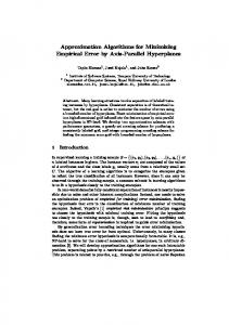
to the proof of k-vertex connectivity in Bredin et al. [2]. G0 is the optimal Steiner graph, that is k-vertex connected on the terminals. Let Gi−1 be k-vertex connected on the terminals. Thus, removal of any set C of k−1 vertices does not disconnect the terminals in Gi−1 . We prove by contradiction that all terminals are connected in Gi − C as well. Let u and v be the two terminals which are disconnected in Gi − C. All terminal pairs (u, v) have a path in Gi−1 − C. If the path does not use more than one terminal connected to component SCi , u and v are connected in Gi − C as well. If the path uses at least two terminal vertices connected to SCi (u1 , v1 being the first and last terminals connected to SCi on the path), that path exists as well if there are at least k + 1 terminals connected to SCi , since we form a Harary graph (that is k-vertex connected) between all terminals connected to SCi . If there are less than k + 1 terminals (which will be u1 , v1 ), a direct edge exists between them (since we formed a complete graph in that case) and thus a path exists between u and v in Gi − C. Thus, Gi is k-vertex connected on terminals. Therefore, by induction, Gm is k-vertex connected on terminals. We now describe the procedure of constructing the Harary graph on terminals connected to each Steiner component SCj . Algorithm 3 describes the algorithm for construction of the kvertex connected graph between terminal nodes connected to the Steiner nodes of STj . The algorithm works as follows: Start at the root of STj (call the root st1 , dropping subscript j for simplicity). Connect to st1 all terminal nodes within its transmission range, and mark them. Let the set of marked terminal nodes be {t1 , .., tl }. Start a Depth First Search (DFS) traversal of the tree formed by STj ∪ {t1 , .., tl } (rooted at st1 ), starting with any child of st1 . The children (both Steiner nodes and terminals) of a node are traversed in an anti-clockwise manner, i.e., the next child to traverse is the first child encountered in an anti-clockwise sweep around the Steiner node, starting from the last child traversed. If no child of the Steiner node has been traversed yet, the child traversed
11 A
1
6
removal
5
of
6
(d) Constructed Harary graph
Example for removal of Steiner nodes and addition of beads for
is the one encountered in the sweep starting from the parent node. Whenever a new Steiner node stj is encountered in the traversal, mark all unmarked terminal nodes in the Steiner node’s transmission range and connect them to it (thus l increases at this step). Figure 1(a) shows an example tree constructed using this procedure for k = 3. While doing the DFS traversal, add required number of beads to form a link between each terminal with the next terminal encountered in the DFS traversal. Complete the cycle by connecting the last added terminal to the first terminal encountered in the DFS traversal2 . Figure 1(b) shows the cycle created between the terminal nodes in the example, starting at terminal 1. Remove the Steiner nodes. Form the Harary graph by connecting each terminal to preceding and successive �k/2� vertices on the cycle, forming a complete graph if there are less than k+1 terminals. The edges longer than unit length are added using the required number of beads. Figure 1(c) shows the constructed cycle after removal of Steiner nodes, and Figure 1(d) shows the final topology (beaded Harary graph) on these terminals nodes. It has been proved in Kashyap et al. [3] that for terminals distributed in the Euclidean plane, the cycle constructed in step 6 of Algorithm 3 contains maximum 5sj beads for each 2 Note that there will be at least two terminals connected to the Steiner nodes of STj . If there were only one terminal node, the Steiner nodes of STj could be deleted from the optimal Steiner graph without affecting the connectivity. In case of two terminal nodes, adding one edge between the two makes it a complete graph, which suffices, as shown before.
Algorithm 3 Removal of Steiner nodes and addition of beads in STj 1: Start at root st1 of STj . 2: Connect to it all terminals within its transmission range, and mark them. 3: Construct a tree Tj , with the vertex set as the Steiner nodes in STj and a leaf vertex corresponding to each marked terminal vertex. The edges are the edges of STj and the edges between each Steiner node and the marked terminal vertices connected to it. 4: Do a Depth First Search (DFS) traversal of Tj rooted at st1 , starting with any child of st1 . For each node, traverse its children in an anti-clockwise manner. 5: Each time a new Steiner node sti is encountered, connect it to all unmarked terminal vertices in its range, and mark them. Update Tj by adding these terminal vertices, and continue DFS traversal around sti from the edge between sti and its parent. 6: Connect all the terminal vertices in order of their DFS traversal and complete the cycle between them. 7: Connect each vertex to preceding and successive �k/2� vertices on the cycle. Form a complete graph if there are less than k + 1 terminals. 8: Add beads to all added edges of length greater than one. 9: Add the newly added edges to Gj−1 , and remove the Steiner nodes of STj and all incident edges from Gj−1 . The resulting graph is Gj . A
E
B
C
D
C
(a) Harary graph
E
E
D
(b) First cycle
C
(c) Second cycle
A
B
D
(d) Third cycle Fig. 2.
• •
A
A
B
and incomplete cycles (we call all of them cycles), and use the result of Kashyap et al. [3] to compute its cost. Let us explain it with an example of Figure 2. Figure 2(a) shows the Harary graph constructed for k = 3, with each terminal connecting to preceding and successive two nodes on the cycle. We decompose the graph into multiple cycles as follows:
B
E
(e) Fourth cycle
Example for decomposition of a Harary graph for k = 3
Steiner component STj with sj Steiner nodes. The analysis only uses the property that the terminals are connected to STj in the Steiner solution. Thus, this result holds for any subset of terminals connected to STj , as long as the cycle is constructed in an anti-clockwise manner. Let the number of terminal nodes in Hj (connected to the Steiner component in consideration) be N . We consider the case N ≥ k + 1, so that we can construct the Harary graph3 . We decompose the constructed Harary graph into complete 3 Else, we construct a complete graph, which is a subset of the set of edges in the Harary graph (since N < k + 1). Thus, the analysis for Harary graph is an upper bound for this case.
•
Type I cycle: First cycle is the cycle formed between all the terminals, as constructed in steps 1-6 of Algorithm 3. Type II cycles: We now consider the edges needed to connect nodes with preceding and successive nodes i hops away (number of edges between the nodes in the Type I cycle) on the Type I cycle into multiple cycles. We start with any terminal node (node A in the example), and form a complete or incomplete cycle by starting with the node and traversing edges that connect nodes i hops away, in an anti-clockwise manner. The cycle ends before or at the node we started at. Figure 2(c) shows the constructed cycle for i = 2. We repeat the procedure for the i − 1 nodes successive to the node we started at (node B in the example, for i = 2), obtaining one complete or incomplete cycle in each case. Figure 2(d) shows this cycle for the example. Each cycle contains N/i edges, and there are i Type II cycles. Each node is connected to one preceding node and one successive node i hops away. Thus, N edges are required to connect all nodes with neighbors i hops away on the Type I cycle. The total edges covered by Type II cycles is i N/i . Thus, to cover the N − i N/i uncovered edges, we form Type III cycles, which are just single edges. Type III cycles: These cycles are single edges, each pertaining to one of the N − i N/i uncovered edges. Figure 2(e) shows the cycle for the example.
There is one Type I cycle in the Harary graph, and i Type II and N − i N/i Type III cycles for each i = 2, 3, .., �k/2�. These cycles cover all the edges in the Harary graph, and thus the number of beads needed for these cycles is the same as needed for the Harary graph. The Type I cycle uses at most 5sj beads. The following lemma bounds the number of beads needed for the Type II edges. Lemma 3.2: A Type II cycle constructed from edges connecting nodes i hops apart requires at most 5sj beads. Proof: Let the set of terminals in the Harary graph be Tj . Let the set of terminals in the Type II cycle be Tj� ⊂ Tj . Consider another instance of the problem, in which only the terminals of Tj� are connected to the Steiner node MST STj . Follow steps 1-6 of Algorithm 3 on this instance to form a cycle. This cycle has at most 5sj beads, Kashyap et al. [3]. The only difference between this instance and the original instance is that the terminals Tj \Tj� have been removed. The order of children traversal in the DFS traversal is anti-clockwise. Removing the terminals Tj \Tj� does not change the order in which the terminals Tj� are encountered (compared to the original instance). Thus, the cycle constructed cycle is the same as the Type II cycle in consideration (or has one extra edge if the Type II cycle is not complete). Thus, the Type II
cycle has at most 5sj beads. Now, we consider the Type III cycles. Each Type III cycle is just an edge. Thus, the required number of beads is at most the number of Steiner nodes in the DFS path between the endterminals of this edge. Thus, a Type III edge requires at most sj beads. Thus, the total number of beads (bj ) required by the Harary graph is as given in Equation 2. �k/2�
bj
�
≤ 5sj +
(5i + N − i N/i )sj
i=2 �k/2�
=
�
5sj +
(5i + i(N/i − N/i ))sj
i=2 �k/2�
≤ 5sj +
�
(6i)sj
i=2 �k/2�
= =
(6
�
i − 1)sj
i=1
(3�k/2�(�k/2� + 1) − 1)sj
(2)
Since the Steiner components SCj do not have common Steiner nodes, the number of beads is at most (3�k/2�(�k/2�+ 1) − 1)s. Thus, a solution with minimum number of beads requires at most (3�k/2�(�k/2� + 1) − 1)s beads. Theorem 3.3 states the main result of this section. Theorem 3.3: If the optimal network uses s Steiner nodes so that terminals distributed in the Euclidean plane are k-vertex connected, Algorithm 1 forms a network with maximum of c(3�k/2�(�k/2� + 1) − 1)s beads and zero Steiner nodes, in which the terminal nodes are k-vertex connected. Proof: The algorithm for finding a k-vertex connected subgraph is a c-approximation for finding the minimum cost k-vertex connected subgraph (cost of each edge being number of beads required to form it). Thus, according to Lemma 3.1, the number of beads required is at most c(3�k/2�(�k/2� + 1) − 1)s. The last step of Algorithm 1 (sequential removal step) removes beads from the network by allowing them to connect to all nodes within the transmission range, so the resulting network after sequential removal also has maximum of c(3�k/2�(�k/2� + 1) − 1)s relay nodes. For k = 2, c is 2, and the algorithm is 10-approximation, which is consistent with the results of Kashyap et al. [3]. IV. A LGORITHM FOR k- EDGE CONNECTIVITY We follow the algorithm proposed by Kashyap et al. [4]. To connect two terminal nodes outside each other’s transmission range, the relay nodes are placed on the straight line connecting the two nodes. The algorithm proceeds by forming a multigraph Gc on the terminal nodes. There are k edges between each pair of terminal nodes in Gc . We use the weight function of Equation 1 to weight the edges. We do not allow the relay nodes to have edges other than the ones required to form the edge they are placed on. Then we compute an approximate
minimum cost spanning k-edge connected subgraph (G�c ) of the multi-graph Gc . The problem of finding the minimum cost spanning kedge connected subgraph of a graph is N P -Hard (Gary and Johnson [13]). Thus, we use an approximation algorithm for the problem, proposed by Khuller and Vishkin [18]. The algorithm achieves an approximation ratio of 2 for the problem, and takes O((kn)2 ) time for a graph with n nodes. The algorithm uses the matroid intersection based algorithm of Gabow [19], which finds k edge-disjoint spanning trees from a root vertex in a directed graph. It is worth noting that the weight function of Equation 1 is not a metric as it does not satisfy triangle inequality. Thus, the approximation algorithm of Khuller and Vishkin [18] is the best known for the problem. In the resulting subgraph from the approximation algorithm of Khuller and Vishkin [18], the relay nodes are placed to form the links (of length greater than one) of the subgraph. In the next section, we prove that this algorithm has an approximation ratio of 2M �k/2�s. The solution is then improved by removing some relays. The relays are allowed to form edges with all nodes in their transmission range and sequentially removed if k-edge connectivity is preserved. We call this step the sequential removal step, and it takes O(n� ((n + n� )m)) time, where n� is the number of relays before the sequential removal step, and m is the number of edges in the network formed by the terminals and relays. Thus, the first part of the algorithm takes O((kn)2 ) time, while the complete algorithm takes O((kn)2 + n� m(n + n� )) time. Algorithm 4 describes the algorithm. For a network in a cuboid of length L, the maximum number of relays on any edge in Gc is O(L), and the number of edges in the graph at the output of Step 3 of Algorithm 4 (G�c ) is k(n−1), thus, n� = O(knL) and m = O((knL)2 ). Therefore, the algorithm takes O((knL)4 ) time. A. Proof of Approximation Ratio We now analyze the algorithm to provide with approximation guarantees. Let the terminal nodes be placed in any metric space with MST number M [6]. MST number is defined as the maximum node degree in a minimum-degree Minimum Spanning Tree (MST) spanning points from the space. The MST number for the Euclidian plane is 5 [5], threedimensional Euclidian space is 12, and rectilinear plane (twodimensional space with metric defined by L1 norm) is 4. The approximation ratio for the MST based algorithm of [9] for connecting terminals using minimum relays has been shown to be M − 1 in [10]. We prove that the algorithm is a 2M �k/2�approximation. We start with some notation. Let T be the set of terminals, and S be the set of optimally placed Steiner nodes (relay nodes) needed to achieve k-edge connectivity among the terminal nodes. Let s be the number of Steiner nodes needed when we place them optimally, i.e, s = |S|. In the proof, we will call the relay nodes placed on straight lines between terminals (as in our algorithm) beads and the optimally placed relay nodes Steiner nodes.
Algorithm 4 Relay placement for k-edge connectivity 1: Make a multi-graph Gc = (V, Ec ) by adding k edges between each pair of vertices of graph G. 2: Weight the edges of the graph as follows. |e| represents the length of edge e. ce = �|e|� − 1 3:
4: 5: 6:
7:
Compute an approximate minimum cost spanning k-edge connected subgraph from this graph Gc using the approximation algorithm proposed by Khuller and Vishkin [18]. Let the resulting graph be G�c . Place relay nodes (number equal to the weight of the edge) on the edges in G�c with link costs greater than zero. For all pairs of nodes (including the relay nodes) in G�c within each other’s transmission range, form an edge. For the relay nodes sorted arbitrarily, do the following (starting at i = 1): • Remove node i (and all adjacent edges). • Check for k-edge connectivity between the terminals. • If the graph is k-edge connected, repeat for i = i + 1, else put back the node i and corresponding edges, and repeat for i = i + 1. • Stop when all relay nodes have been considered. Output the resulting graph.
As a recap of our algorithm, it forms a k-edge connected network among the terminal nodes by placing additional links between them, and if two terminal nodes are more than unit distance apart, it adds beads (relay nodes) to form that link. When we add such a link of length l, it consists of �l� − 1 beads. We first prove the following lemma, and then the main result of this section. Lemma 4.1: A k-edge connected network on terminal nodes using minimum number of beads contains at most M �k/2�s beads, where s is the minimum number of Steiner nodes needed. Proof: Let G0 = (V0 , E0 ) be the optimal k-edge connected network on terminals (having the minimum number of Steiner nodes). We follow a slightly modification of Algorithm 2 to construct a k-edge connected network that has beads and no Steiner nodes. We will prove that this network does not contain more than M k beads. The algorithm starts by finding the connected components (SCi ) of Steiner nodes in the graph constructed on the Steiner nodes. It constructs a Breadth First Search (BFS) spanning tree on Steiner nodes for each connected component, starting with any Steiner node in that component as the root. Let the trees be ST1 , .., STm . The algorithm then removes Steiner nodes of a connected component SCj from Gj−1 and adds beads between the terminals connected to those Steiner nodes to get Gj which is also k-edge connected between terminal nodes (Step 4). The process is repeated for all connected components,
and the resulting graph has zero Steiner nodes and is k-edge connected on the terminals. Let us now explain the procedure to construct Gj from Gj−1 by adding beads between the terminal nodes and removing Steiner nodes. Consider the graph formed by the Steiner nodes in STj and the terminal nodes within the transmission range of these Steiner nodes. Denote this graph by Hj . We form a cycle among the terminals in Hj , and replicate the edges to have �k/2� copies of each. We use beads to form the edges longer than unit length. The terminals in Hj are k-edge connected since deleting any set of k − 1 edges does not disconnect the terminals from each other. This procedure maintains kedge connectivity between the terminal nodes that were k-edge connected because of the Steiner nodes in STj . As we do this for all trees ST1 , .., STm 4 , and do not create any (k − 1)-edge cut in any step, the resulting network is k-edge connected on the terminals. It has been proved in Kashyap et al. [4] that the constructed cycle contains at most M sj beads for each Steiner component STj with sj Steiner nodes. We replicate the edges to include �k/2� − 1 additional copies of each edge, and thus the graph uses M �k/2�sj beads. Since the Steiner components do not have common Steiner nodes, total number of beads required is bounded by M �k/2�s. Theorem 4.2 states the main result of this section. Theorem 4.2: If the optimal network uses s Steiner nodes so that terminals distributed in metric space of MST number M are k-edge connected, Algorithm 4 forms a network with maximum of 2M �k/2�s beads and zero Steiner nodes, in which the terminal nodes are k-edge connected. Proof: The algorithm of Khuller and Vishkin [18] is a 2approximation for finding the minimum cost (cost of each edge being number of beads required to form it) k-edge connected subgraph. Thus, the number of beads required is at most 2M �k/2�s. The last step of Algorithm 4 (sequential removal step) removes beads from the network by allowing them to connect to all nodes within the transmission range, so the resulting network after sequential removal also has at most 2M �k/2�s relay nodes. Note that for k = 2, the algorithm is a 2M -approximation, which is consistent with the ratio proved in Kashyap et al. [4]. V. G ENERALIZATION TO R ESTRICTED R ELAY P LACEMENT We extend our results for terminals distributed in a Euclidian plane to the scenario where relays cannot be placed in certain polygonal regions of the network . We call these regions forbidden regions. We assume that two nodes can communicate if they are within each other’s transmission range even when there is a forbidden region between them. We modify the edge and vertex connectivity algorithms to work with the same approximation guarantees for this generalization. We follow the same algorithms as before for both edge connectivity and vertex connectivity. It may not be possible 4 If two terminal nodes are adjacent in multiple cycles formed while removing the Steiner components, we form maximum k beaded links between them. This suffices for maintaining k-edge connectivity.
to connect two terminals by placing relay nodes on the straight line between them due to the forbidden regions. Thus, Equation 1, which represents the number of relays needed to connect two terminals by placing relays on the line between them, cannot be used to weight the edges of the network formed on terminal nodes in our algorithms. Recently, a polynomial time algorithm has been proposed for placing the minimum number of relay nodes needed to form a link between two nodes with the presence of polygonal forbidden regions between them [20] . The problem is called the puddlejumper problem. We modify our edge weights by running the algorithm given in [20] on each pair of terminals in the network to find the minimum number of relay nodes needed for each link, and using that as the weight of each edge. We then run our edge connectivity and vertex connectivity algorithms on a network with these edge weights. Then, for the selected links, we place the relays according to the algorithm given in [20]. A. Proof of Approximation Ratio We first prove that the approximation ratio for the k-vertex connectivity algorithm is O(k2 ) for terminals distributed in the Euclidian plane. We follow the same construction as before, the only change being that beads (relay nodes) are not placed on straight lines between terminal nodes now; instead they are placed optimally taking forbidden regions into account. The only part of the proof that needs reconsideration to take forbidden regions into account is when Steiner nodes on a tree (STj ) are removed from the optimal Steiner solution and beads are placed to make the cycle (and the Harary graph) between terminal nodes connected to tree STj (see Algorithm 3). We argue that the number of relays needed to form a beaded link between two terminals is still upper bounded by the number of Steiner nodes encountered in the depth first traversal between the two terminals: Take any two terminals being connected using beads, and let a be the number of Steiner nodes on the DFS path between them. Thus, there is a placement of Steiner nodes to connect the two terminal nodes using a Steiner nodes. As even Steiner nodes could not be placed in forbidden regions, and we connect the terminals using beads placed according to the optimal algorithm of [20], the number of beads required is upper bounded by a. Thus, each bead can still be charged to a different Steiner node on the DFS path between the terminals. We showed in Section IV that each Steiner node is charged at most (3�k/2�(�k/2� + 1) − 1) times (M = 5 for Euclidian plane), so the total number of beads required for replacing the Steiner node tree STj is still (3�k/2�(�k/2� + 1) − 1)sj , sj being the number of Steiner nodes in STj . Thus the total number of beads required in the network is at most (3�k/2�(�k/2� + 1) − 1)s for the beaded network using minimum number of beads, s being the number of optimal Steiner nodes. As our algorithms use c-approximations (c = 2 for edge-connectivity) for finding the optimal beaded network, the algorithms are c(3�k/2�(�k/2�+ 1) − 1)s-approximations.
The same arguments can be used to prove that the edgeconnectivity algorithm is 10�k/2�-approximation for this generalization (c = 2 for edge-connectivity, and M = 5 for Euclidean plane). VI. F ULL k-C ONNECTIVITY We now present the algorithms and analysis for achieving k-vertex and k-edge connectivity between terminals and added relays. We first discuss k-vertex connectivity. A. Full k-vertex connectivity We use the algorithm proposed in Bredin et al. [2]. The algorithm adds relays to find a subgraph on terminals that is k-vertex connected on terminals using the algorithm presented in Section III. Then, for each edge of the k-connected subgraph with weight greater than zero, i.e., with at least one relay, the algorithm places additional k − 1 relays at each of the end terminal vertices of the edge, and k − 1 relays along with each relay used on the edge. In the resulting graph, all terminals and relays have k-vertex connectivity. The algorithm has been proved to have an approximation ratio of O(k4 ) for terminals in Euclidean plane. We improve the analysis, and prove the algorithm to be an O(k3 )-approximation. Theorem 6.1 states the result. Here, c is the approximation ratio of the best algorithm for finding a k-vertex connected subgraph of a graph. Theorem 6.1: If the optimal network uses s Steiner nodes so that terminals and Steiner nodes are k-vertex connected, the algorithm of Bredin et al. [2] forms a network with at most 3c(3�k/2�(�k/2� + 1) − 1)ks relays and zero Steiner nodes, in which the terminal and relay nodes are k-vertex connected. Proof: The optimal network that is k-vertex connected only on terminals uses s Steiner nodes. Thus, according to Theorem 3.3, the intermediate graph that is k-vertex connected on terminals has at most c(3�k/2�(�k/2�+1)−1)s relays. As shown in Bredin et al. [2], for each edge between terminals with w ≥ 1 relays, we duplicate them to have a total of kw + 2(k − 1) < 3kw relays on the edge. Thus, the total number of relays in the final fully k-vertex connected graph is bounded by 3c(3�k/2�(�k/2� + 1) − 1)ks, which is an O(k 3 )-approximation, an O(k) improvement over the previous bounds of Bredin et al. [2]. B. Full k-edge connectivity For edge connectivity, we use the algorithm presented in Section IV. We use the algorithm to construct a k-edge connected subgraph on terminals, and then duplicate the relays needed on the edges of that subgraph. For each edge of weight greater than zero, we place additional �k/2� − 1 relays at each end terminal vertex of the edge, and each relay location on that edge. The resulting graph is k-edge connected on both terminals and relays. We prove the algorithm is an O(M k2 )approximation for terminals distributed in a metric space of MST number M . Theorem 6.2 states the result. Theorem 6.2: If the optimal network uses s Steiner nodes so that terminals and Steiner nodes are k-edge connected, our
algorithm forms a network with at most 6M �k/2�2 s relays and zero Steiner nodes, in which the terminal and relay nodes are k-edge connected. Proof: The optimal network that is k-edge connected only on terminals uses s Steiner nodes. Thus, according to Theorem 4.2, the intermediate graph that is k-edge connected on terminals has at most 2M �k/2�s relays. Then, for each edge between terminals with w ≥ 1 relays, we duplicate them to have a total of �k/2�w + 2(�k/2� − 1) < 3�k/2�w relays on the edge. Thus, the total number of relays in the final fully k-edge connected graph is bounded by 6M �k/2�2 s. VII. C ONCLUSION We considered the problem of constructing a fault-tolerant topology among sensor nodes using minimum number of additional relay nodes. We proposed O(k2 )-approximation algorithms for achieving k-vertex connectivity between sensor nodes distributed in the Euclidean plane. We proposed 2M kapproximation algorithms for achieving k-edge connectivity between terminal nodes distributed in any metric space with MST number M . We extended our algorithms to work with the same approximation guarantees for the generalization where the relay nodes cannot be placed in certain polygonal regions of the network. We analyzed an existing algorithm proposed for achieving k-vertex connectivity between sensor nodes and relays using minimum number of relays, and proved it to have an approximation guarantee of O(k3 ), which is an O(k) improvement over previously proved bounds. We also proposed an algorithm for achieving k-edge connectivity between sensor nodes and relays using minimum number of relays, and proved it to have an approximation guarantee of O(M k 2 ). R EFERENCES [1] I. F. Akyildiz, W. Su, Y. Sankarasubramaniam, and E. Cayirci, “Wireless sensor networks: a survey,” Computer Networks, vol. 38, no. 4, pp. 393– 422, 2002. [2] J. L. Bredin, E. D. Demaine, M. Hajiaghayi, and D. Rus, “Deploying sensor networks with guaranteed capacity and fault tolerance,” ACM MobiHoc, pp. 309–319, 2005. [3] A. Kashyap, S. Khuller, and M. Shayman, “Relay placement for higher order connectivity in wireless sensor networks,” IEEE INFOCOM, 2006. [4] ——, “Relay placement for fault-tolerance in wireless sensor networks in higher dimensions,” submitted to ACM Trans. Sensor Networks, 2006. [5] C. Monma and S. Suri, “Transitions in geometric minimum spanning tree,” Discrete and Computational Geometry, vol. 8, pp. 265–293, 1992. [6] G. Robins and J. S. Salowe, “Low-degree minimum spanning trees,” Discrete Computational Geometry, vol. 14, pp. 151–165, 1995. [7] B. Hao, J. Tang, and G. Xue, “Fault-tolerant relay node placement in wireless sensor networks: Formulation and approximation,” IEEE HPSR, pp. 246–250, 2004. [8] H. Liu, P. Wan, and X. Jia, “Fault-tolerant relay node placement in wireless sensor networks,” International Computing and Combinatorics Conference (COCOON), 2005. [9] G.-H. Lin and L. Wang, “Steiner tree problem with minimum number of Steiner points and bounded edge-length,” Information Processing Letters, vol. 69, pp. 53–57, 1999. [10] I. Mˇandoiu and A. Zelikovsky, “A note on the mst heuristic for bounded edge-length Steiner trees with minimum number of Steiner points,” Information Processing Letters, vol. 75, no. 4, pp. 165–167, 2000. [11] D. Chen, D.-Z. Du, X.-D. Hu, G.-H. Lin, L. Wang, and G. Xue, “Approximations for Steiner trees with minimum number of Steiner points,” Theoretical Computer Science, vol. 262, pp. 83–99, 2001.
[12] X. Cheng, D.-Z. Du, L. Wang, and B. Xu, “Relay sensor placement in wireless sensor networks,” ACM Winet, 2004. [13] M. Garey and D. Johnson, Computers and Intractability: A guide to the theory of NP-Completeness. Freeman and Company, 1979. [14] S. Khuller and B. Raghavachari, “Improved approximation algorithms for uniform connectivity problems,” Journal of Algorithms, vol. 21, no. 2, pp. 434–450, 1996. [15] G. Kortsarz and Z. Nutov, “Approximating node connectivity problems via set covers,” Algorithmica, vol. 37, pp. 75–92, 2003. [16] V. Auletta, Y. Dinitz, Z. Nutov, and D. Parente, “A 2-approximation algorithm for finding an optimum 3-vertex connected spanning subgraph,” Journal of Algorithms, vol. 32, pp. 21–30, 1999. [17] Y. Dinitz and Z. Nutov, “A 3-approximation algorithm for finding optimum 4,5-vertex connected spanning subgraphs,” Journal of Algorithms, vol. 32, pp. 31–40, 1999. [18] S. Khuller and U. Vishkin, “Biconnectivity approximations and graph carvings,” Journal of the ACM, vol. 41, no. 2, pp. 214–235, 1994. [19] H. N. Gabow, “A matroid approach to finding edge connectivity and packing arborescences,” IEEE Annual Symposium on Foundations of Computer Science, pp. 812–822, 1991. [20] E. Arkin, E. Demaine, and J. Mitchell, “The puddle-jumper problem,” Personal Communication, 2005.