Reliability Based Design Optimization of Robotic System ... - CiteSeerX

06M-264

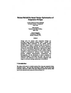
Reliability Based Design Optimization of Robotic System Dynamic Performance Alan Bowling, John E. Renaud, Neal M. Patel, Jeremy Newkirk University of Notre Dame, Notre Dame, Indiana, 46556, USA

Harish Agarwal General Electric Global Research, Niskayuna, New York, 12309, USA c 2005 SAE International Copyright °

ABSTRACT

reference point on the robot’s end-effector to evaluate the performance measure. These performance measures are not invariant to the choice of this reference point on the end-effector referred to as the operational point (16). Thus the measures predict different levels of performance for different operational points, and those predictions are not equivalent. The measure is said to not be invariant to origin choice. However, depending on the tool used for the end-effector, the operational point can change. Thus it is desirable to design the robot in a manner which addresses this variation in use, or uncertainty with respect to the operational point, thereby also addressing the invariance to origin issue discussed in (16).

In this investigation a robotic system’s dynamic performance is optimized for high reliability under uncertainty. The dynamic capability equations allow designers to predict the dynamic performance of a robotic system for a particular configuration (i.e.,point design). While the dynamic capability equations are a powerful tool, they can not account for performance variations due to aleatory uncertainties inherent in the system. To account for the inherent aleatory uncertainties, a reliability-based design optimization (RBDO)strategy is employed to design robotic systems with robust dynamic performance. RBDO has traditionally been implemented as a nested multilevel optimization process in which reliability constraints require solution to an optimization problem (i.e., reliability analysis). In this work a robust unilevel performance measure approach(PMA) is developed for performing reliability-based design optimization which eliminates the lower level problem in RBDO. A robotic test problem is used to illustrate the efficacy of the approach.

One way of addressing the invariance issue is to sample various operational points and attempt to perform statistics on those samples in order to satisfy some average, minimum, or maximum performance. A different strategy utilizes an optimization scheme referred to as Reliability Based Design Optimization (RBDO) which uses probability density functions to characterize the region of feasible operational points. Within the overall actuator selection optimization, invariance to origin is addressed by examining this region in order to determine the operational point with the highest probability of having the worst performance. A key point is that when using RBDO this examination is accomplished without sampling the region.

INTRODUCTION The focus of this research is to study the model-based, or simulation-based, design of robotic systems while accounting for the uncertainty in the modes of use for the design. Oftentimes a general purpose robot is not used in the mode which was the basis for the design. This is especially true for robots whose design focuses on dynamic performance. This refers to a robotic manipulator’s ability to accelerate its end-effector and to apply forces/moments to the environment at the endeffector. There are several dynamic performance measures and characterizations currently available in the literature including (30; 13; 20; 7). These performance measures and characterizations are usually used along with optimization techniques to drive the choice of various design parameters, such as link lengths and actuator sizes. In this work, the actuator selection problem is based on the dynamic capability equations (DCE) developed in (7) which are used in an optimization to find actuators that will provide a desired level of dynamic performance.

Historically uncertainties have been addressed using safety factors,where the designer simply over-designs or under-designs the system in an effort to account for the variations. However, depending on the complexity of the system, this approach may not be adequate. The goal of this work is to address these uncertainties by including them in the model upon which the design is based. This approach yields a more systematic treatment of the uncertainties than is possible using safety factors. The sensitivity to choice of operational point can be minimized and controlled, yielding a more reliable robot. Reliability has often been associated with failure of a robot in some manner and there is much recent work in this area. A popular area concerns addressing joint failure from the standpoint of analysis (27), design (15), and control (4) of robotic manipulators. Each paper references several other works on this topic. Although the language of RBDO, with respect to failure modes and such, has much in common with these works on fault tol-

However, an issue common among most performance measures, and those in (30; 13; 20; 7) in particular, must be evaluated at a particular configuration using a particular choice of 1

erance, the application here is somewhat different. The fault or failure with respect to a malfunction of the system, but more aligned with meeting or not meeting design goals. The work in (3) is closer to the work presented here because probabilistic methods are used to estimate the positioning and orienting accuracy for the end-effector of a robotic manipulator. Assuming that all kinematic parameters of the robot are Gaussian distributions, the paper attempts to determine the probability that the end-effector will lie within some given region of the desired position and orientation. This work resulted in an analytical solution to the problem which could be obtained using simple probability density functions. However, this work and others like it are more suited to addressing variations due to manufacturing rather than variation due to use considered here.

This is done by specifying all of the terms on the left-hand-side of (1), including the configuration q, and determining the torque required to produce those specified motions. The dynamic capabilities are specified in a manner that allows each constraint to maintain homogeneous units, v T v = |v|2

F T F = |F|2

ω˙ T ω˙ = |ω| ˙ 2

ω T ω = |ω|2

MT M = |M|2 .

(3)

|v| ˙ represents the balanced translational acceleration, which ˙ and likewise for the other terms of bounds the magnitude kvk, the form | · |. In general, each of these relations represents a sphere.

Υ1

In the following sections the DCE and its use in the actuator selection problem is discussed first. This is followed by a discussion of reliability based optimization. Finally the method is applied to actuator selection for a two degree-of-freedom (DOF) planar manipulator.

E |v| ˙

Υ2

DYNAMIC PERFORMANCE AND ACTUATOR SELECTION

actuator space

The analysis of dynamic performance, the DCE, used in the proposed work was originally developed for fixed-base robotic manipulators. The DCE is a recent development which is used here for two reasons: 1) it is one of the few robot performance analyses to treat translational and rotational quantities in a manner that is consistent, physically meaningful, and satisfies all aspects of invariance except invariance to origin (11; 16) and 2) it is also one of the very few to unify the consideration of many different aspects of dynamic performance including accelerations, forces, and velocities. Dynamic performance is limited by the amount of torque the robot’s actuators can produce. Since all aspects of dynamic performance are related to actuator torque through the equations of motion, it is possible to unify the analysis of these quantities and to determine the relationship between them.

end-effector acceleration space

Figure 1: Analysis of Manipulator Performance. This analysis is best understood by considering a simple example, the two DOF planar robotic manipulator shown in Fig. 1. The equations of motion for this case are E v˙ + g = Υ.

(4)

The acceleration is specified as a circle with radius |v|, ˙ and the mapping of acceleration to actuator torque is expressed as ¡ ¢−1 v˙ T v˙ = |v| ˙ 2 −−−−−−−→ Υv˙T E E T Υv˙ = |v| ˙ 2 . (5) E v˙ = Υv˙ The term of the left-hand-side of (5) is represented by the solid circle in the end-effector acceleration space of Fig. 1. The righthand-side of (5) describes the actuator torques required to produce the circle of accelerations, represented by the solid ellipse in actuator space; see Fig. 1.

The DCE for a fixed-base robotic manipulator are obtained from the equations of motion expressed as, ¸ · ¸ · v˙ f + E(q) + C(q, v, ω) + g(q) = Υ, (1) E(q) ω˙ m

The actuator torque bounds represent the available torque, shown as the square in actuator space. The image of these bounds in end-effector acceleration space is shown as the acceleration parallelepiped (19) or polytope. The ellipse is compared against the available torque by expanding it until it touches the torque bounds. The extent of the balanced translational acceleration, |v|, ˙ is determined by the largest ellipse that can be inscribed within the parallelepiped. This gives the largest magnitude of translational acceleration achievable in every direction. The isotropic or balanced accelerations has often been used to analyze acceleration capability (19; 30; 13; 20).

n

and the bounds on the actuator torques, Υ ∈ R , expressed as −Υbound ≤ Υ ≤ Υbound

v˙ T v˙ = |v| ˙2

(2)

where q ∈ Rn is a vector containing the generalized coordinates of the model, which define the configuration or posture of the manipulator. v and v˙ are the translational velocity and acceleration of the operational point on the end-effector, while ω and ω˙ are the rotational velocity and acceleration of the endeffector. The vectors f and m represent end-effector contact forces and moments. The terms E(q) ∈ Rn×n , E(q) ∈ Rn×n , g(q) ∈ Rn , and C(q, v, ω) ∈ Rn are the inertial properties, transmission between end-effector and actuator forces, gravity forces, and the Coriolis and centrifugal forces and other velocity dependent terms. The vector Υbound ∈ Rn contains the limits on the amount of torque each actuator can supply.

The side of the acceleration parallelepiped in contact with the balanced acceleration circle indicates the limiting actuator, the actuator which saturated attempting to provide the balanced translational acceleration. The vector in Fig. 1, which indicates the contact point between the circle and parallelepiped, represents the worst-case direction of acceleration. Note that in every other direction an equal or larger amount of acceleration is achievable. Thus the balanced translational acceleration is also interpreted as the worst-case acceleration achievable from the given configuration.

The underlying idea here is to compare the actuator torques required to produce balanced or isotropic acceleration and force capabilities, to the total available actuator torques defined by the bounds in (2). 2

˙ = |v| = |ω| = 0, a second section of the hypersurface where |ω| which illustrates the relationship between acceleration capability and contact forces. This surface is comprised of many facets, which means that different actuators, indicated by the numeric labels on each surface patch, saturated attempting to provide the performance described by the surface. Notice that the accelerations are driven to zero as the contact forces and moments increase.

Fig. 1 also shows other approaches towards analyzing acceleration capability. The dashed circle and ellipse in Fig. 1 represent the well known Dynamic Manipulability Ellipsoid; (30; 9; 8). There are several other approaches to describing the acceleration and force capabilities of robotic manipulators, including examination of the end-effector inertial properties of the system in order to describe the difficulty of accelerating in a different directions; (17; 29; 18; 2; 21; 23; 28). However, the above studies mixed units of translational and rotational motion in their descriptions of acceleration capability such that they were not invariant to changes in units.

The DCE and DCH describe the robot’s dynamic performance given a set of actuator torques. The inverse problem is to specify a desired dynamic performance and to determine the actuator torques that will provide that level of performance. This is the actuator selection problem discussed in (5; 6). The desired performance is specified by describing the desired shape of the DCH using performance points of the form

Another feature of the DCE approach is that it allows for the unification and comparison of different dynamic capabilities, because all quantities are mapped into actuator torque. Very few studies take this approach excepting (20; 12) which considered accelerations and velocities together. This unification allows a study of forces and velocities to be carried out within the context of dynamic performance. These quantities are usually studied from a kinematic viewpoint.

pi = ( |v| ˙ i , |ω| ˙ i , |f|i , |m|i , |v|i , |ω|i ) .

Actuators are then chosen such that the DCH encompasses all of the performance points.

The DCE have the following form " # " # " # ¡ 2 ¢ |v| ˙ |f| Υbound 2 A + C |v| , |ω| + F ≤ −G = T, |ω| ˙ |m| Υbound (6) which describe the six-dimensional Dynamic Capability Hypersurface (DCH). G is the vector of gravity terms. There is a very simple transformation involved in obtaining the A and F matrices from (5). It is more difficult to obtain the C vector because the velocity terms are nonlinear, versus the linear acceleration and force terms. However, it is still possible to analyze the velocity terms without resorting to a purely numerical approach.

The basic idea is to substitute these points into the DCE, (6), in order to determine whether the specified performance is feasible or not. The resulting relations act as constraints on the optimization problem. This was accomplished for a particular operational point and configuration in (6). The optimization problem was formulated as: where the desired performance, |v| ˙ i , |ω| ˙ i, min

Υbound , αi

subject to

v˙

In the proposed approach, actuators are selected which take into account the variation in use due to an uncertain operational point. The RBDO finds actuators that will satisfy the performance constraints to within a certain probability of failure. This means that some percentage of the points within the range of uncertainty will not be able to satisfy the performance point(s). Inability to achieve the performance point is the dominant failure mode in actuator selection. The probability of failure and failure modes are discussed further in Sec. .

10

v

0 0 0.1

2

0.2

|v |

0.3

4

6

8

|v˙ |

/s

m

(a)

0

|v˙ |

2 /s m

m/s 2

(b)

5

5

2

0

1 50

4

100

6 8

|F |

¸ |v| ˙i + αi2 C(|v|2i , |ω|2i ) ˙ i ¸ · |ω| · ¸ |f|i Υbound + αi F + G − ≤0 |m|i Υbound ·

|f|i , |m|i , |v|i , |ω|i , is given. The objective in this problem is to find the optimum values of the motor torques and the scalar αi that minimizes the weighted sum of torques and satisfies the performance constraints. The transformation of this deterministic optimization problem into an RBDO form is shown explicitly in Sec. .

15

2

Υboundn Υminn

(8)

|M| N m

2

+ ··· +

αi ≥ 1

60

20

Υbound1 Υmin1

Υmin ≤ Υbound ≤ Υmax

˙ ω 40

Cost =

giR = αi A

The largest possible values of the variables in the Dynamic Capability Equations define what is referred to as the Dynamic Capability Hypersurface. Since the six-dimensional hypersurface is difficult to visualize, three-dimensional sections of it are examined in order to investigate its properties. A section of the hypersurface, obtained by setting |ω| = |f| = |m| = 0 in (6), is shown in Fig. 2a for the PUMA 560 manipulator, at the configuration shown in Fig. 2b. The surface represents the largest values of |v|, ˙ |ω| ˙ and |v| which satisfy the relations in (6). Notice in Fig. 2a that the balanced accelerations go to zero as velocity increases.

|ω| ˙ rad/s2

(7)

N

(c)

Figure 2: PUMA 560 Dynamic Capability Hypersurface Sections.

RELIABILITY BASED OPTIMIZATION OPTIMIZATION UNDER UNCERTAINTY

The hypersurface displays the magnitudes of the worst-case combinations of acceleration, velocity and contact forces and moments. The actuator that saturated, or reached its maximum torque, for the worst case is indicated by the numeric label on the surface of Fig. 2a. The motion directions corresponding to this worst case are indicated by the line segments emanating from the end-effector of the PUMA 560 in Fig. 2b. Fig. 2c shows

Uncertainties are inherently present in the simulation-based design of robotic systems. Over the last few years there has been an increased emphasis focused on accounting for the various forms of uncertainties that are introduced in mathematical models and simulation tools. In general, a distinction can 3

be made between aleatory uncertainty (also referred to as stochastic uncertainty, irreducible uncertainty, inherent uncertainty, variability), epistemic uncertainty (also referred to as reducible uncertainty, subjective uncertainty, model form uncertainty or simply uncertainty ) and numerical uncertainty (also known as error) (25; 24; 26). This research focuses on reliability-based design optimization in which aleatory uncertainties are considered. Previous efforts by the PI have focused on accounting for epistemic uncertainty in simulation-based design optimization (1). In this research reliability analysis provides the basis for evaluating the probability of failure of a system.

In this investigation an improved RBDO formulation will be developed for use with the Dynamic Capability Equations to produce reliable optimal designs for robotic systems. A new computationally effecient unilevel formulation for RBDO will be developed that exhibits improved efficiencies and numerical stability. Nested Optimization in RBDO Traditionally, the reliability based optimization problem has been formulated as a double-loop or nested optimization problem. In a typical RBDO formulation, the critical hard constraints are replaced by reliability constraints, as shown below

Reliability Analysis Using Probability Theory Reliability analysis is a tool to compute the reliability index or the probability of failure corresponding to a given failure mode or for the entire robotic system (14). Letting giR (X, η ) ≤ 0 represent the failure domain and giR (X, η ) = 0 be the so-called limit state function, then the time-invariant probability of failure for the ith hard constraint is given by Z η Pi (η ) = fX (x) dx (9)

minimize : subject to :

where fX (x) is the joint probability density of X. It is almost impossible to find an analytical solution to the above integral. In standard reliability techniques, a probability distribution transformation T : Rn → Rn is usually employed. An arbitrary n-dimensional random vector X = (X1 , X2 , ..., Xn )T is mapped into an independent standard normal vector U = (U1 , U2 , ..., Un )T . The standard normal random variables are characterized by zero mean and unit variance. The limit state function in U-space can be obtained as giR (x, η ) = giR (T (u), η ) = GR i (u, η ) = 0. The failure domain in U-space (u, η ) ≤ 0. Equation (9) thus transforms to is GR i Z Pi (ηη ) = φU (u) du (10)

girc g rc

= Pallowi − Pi i = 1, .., Nhard = Pallowsys − Psys

(18) (19)

where Pi is the failure probability of the hard constraint giR at a given design and Pallowi is the allowable probability of failure for this failure mode, Psys is the system failure probability at a given design and Pallowsys is the allowable system probability of failure. It should be noted that the RBDO formulation given above (Equations (13)-(17)) assumes that the violation of soft constraints due to variational uncertainties are permissible and can be traded off for more reliable designs. For practical problems, design robustness represented by the merit function and the soft constraints could be a significant issue, one that would require solution to a hybrid robustness and reliability based design optimization formulation.

η GR i (u,η )≤0

where φU (u) is the standard normal density. In the following, the index i and parameters η are omitted whenever necessary without any loss of clarity. If the limit state function is close to αT u∗ , where being linear i.e., if GR (u, η ) ≈ α T u + β with β = −α ∗ u is the solution of the following optimization problem, |uk GR (u, η ) = 0

j = 1, .., Nsof t

(13) (14) (15) (16) (17)

where grc represents reliability constraints. They are either constraints on probabilities of failure corresponding to each hard constraint, or a single constraint on the overall system probability of failure. grc can be formulated as follows.

η )≤0 giR (x,η

minimize : subject to :

f (d, p, y(d, p)) grc (x, η ) ≥ 0 gjD (d, p, y(d, p)) ≥ 0 h(d, p, y(d, p) = 0 dl ≤ d ≤ du

The probabilities of failure are usually estimated by employing standard reliability techniques as detailed in (14). It is extremely difficult to exactly calculate the probability of failure corresponding to a failure mode. Therefore first order approximations to the limit state functions are generally employed and an estimate of the probability of failure can be found using FORM which is accurate for most practical cases. Using the first order approximation, the reliability constraints in Equation (18) can be reformulated as shown below

(11) (12)

then the first order estimate of the probability of failure is Pf = Φ(−βp ), where α represents the vector of direction cosines at the solution point. The solution u∗ of the above optimization problem, the so called design point, β-point or the most probable point (MPP) of failure, defines the reliability index α∗ u∗ . βp is a signed reliability index. It is positive if βp = −α the origin in U-space is contained in the feasible region i.e. GR (0, η ) > 0, and vice versa. This method of estimating the probability of failure is known as the first order reliability method (FORM) (14). In the second order reliability method (SORM), a second order approximation to the limit state surface is used to estimate the probability of failure.

girc = βi − βreqdi

i = 1, .., Nhard

(20)

where βi is the first order reliability index and βreqdi = −Φ−1 (Pallowi ) is the desired reliability index for the ith hard constraint.

Reliability Index Approach (RIA) When the reliability constraints are formulated as given in equation (20), the approach is referred to as the reliability index approach (RIA). The reliability index corresponding to a failure mode requires solution to an optimization problem as given in equations (11-12). The solution typically requires many system

Reliability-Based Design Optimization (RBDO) Reliability based design optimization (RBDO) deals with finding optimum designs that satisfy a probability of failure constraint. 4

subject to

analysis evaluations. Moreover in RIA, there might be cases where the optimizer may fail to provide a solution to the FORM problem, especially when the limit state surface is far away from the origin in U-space or when the case GR (u, η ) = 0 never occurs at a particular design variable setting.

h(d, p, y(d, p)) = 0 dl ≤ d ≤ du

Performance Measure Approach (PMA)

(21)

and GR,∗ is the solution to the following inverse reliability analyi sis (IRA) optimization problem GR i (u, η ) kuk = ρ where ρ = βreqdi

(22) (23)

where u∗i is the optimum (corresponding MPP in IRA) of the ith hard constraint. Solving RBDO by the PMA formulation is usually more efficient and robust than the RIA formulation, where the reliability is evaluated directly. The efficiency lies in the fact that the search for the MPP of an inverse reliability problem is easier to solve than the search of the MPP corresponding to an actual reliability.

EXAMPLE: ACTUATOR SELECTION In order to illustrate the proposed methodology, in this section a unilevel RBDO is performed on a simple two degree-of-freedom planar manipulator, shown in Fig. 3, which is similar to the one discussed in conjunction with Fig. 1. In this example, the variation in the location of the operational point is considered, however it is assumed that the end effector is rigidly attached to the end of the second link. This variation corresponds to the notion that the location of the end-effector and operational point depend on choices made by the user. These choices cannot be known at the design stage when building a general purpose robot. However, it is important that this uncertainty is accounted for within optimization.

A Unilevel PMA Method for RBDO of Robotic Systems

2

The initial focus of this research will be to develop an efficient and robust unilevel PMA formulation for performing RBDO for the reliablility based design optimization of robotic systems. As mentioned earlier, the probabilistic constraint evaluated by using the performance measure approach is robust compared to the reliability index approach. However, the methodology is still nested and is hence expensive, especially for large problems. In this research, the inverse reliability analysis (IRA) optimization problem that is used to evaluate the probabilistic constraints in the performance measure approach is replaced by the corresponding first order necessary Karush-Kuhn-Tucker (KKT) optimality conditions. It should be noted that the KKT condition for the FORM problem and the IRA problem differs only in terms of what constraints are being presented as equality constraints to the optimizer. When using the KKT conditions of the FORM problem in the upper level optimization, the limit state function is presented as an equality constraint and the constraint on the reliability index is an inequality constraint. As mentioned earlier, it is possible to have cases where the limit state function never becomes zero. In other words, it is associated with zero failure probability. When such a case occurs, the method given by (22) might fail. Hence, in the proposed method, the KKT conditions for the reliability constraints obtained in PMA are used. The corresponding KKT conditions for the inverse reliability problem (Eqns. (22)-(23) ) are as follows

L3 L4

q2 L1

q1

Figure 3: Two DOF Robot Design Problem. A deterministic actuator design problem can be formulated for the manipulator in Fig. 3 as given in Eq. (33), where the desired performance, |v| ˙ i , |ω| ˙ i , |F|i , |M|i , |v|i , |ω|i , is given. The objective in this problem is to find the optimum values of the motor torques and the scalar αi that minimizes the weighted sum of torques and satisfies the performance constraints. The main parameters in the problem are the link lengths, joint angles, link masses and moments of inertia. The suitable values for these are shown is Table 1. The desired level of performance is spec-

Using these first order optimality conditions, the unilevel RBDO formulation can be stated as follows min

:

f (d, p, y(d, p))

k Lin 1

L2

T R h1i (ui , η ) ≡ kui k k∇u GR i (ui , η )k + ui ∇u Gi (ui , η ) = 0 (24) h2i (ui ) ≡ kui k − βreqdi = 0 (25)

daug =(d,u1 ,..,uNhard )

(31) (32)

Link

minimize : subject to :

(27) (28) (29) (30)

It should be noted that the dimension of the problem has increased. The optimization needs to be performed with an augmented design variable vector daug which consists of the design variables d and the MPPs of each hard constraint u∗i . At the beginning of the optimization, ui does not correspond to the true MPP at the design d. The exact MPPs u∗i and the optimum design d∗ are found at the very end of the optimization i.e., when convergence is achieved. Also note that the limit state function is presented as an inequality constraint, as in PMA and therefore the proposed unilevel formulation is robust. The proposed formulation satisfies the constraint qualification of the KKT conditions which is important to insure a unilevel formulation that is mathematically equivalent of the bilevel PMA. More importantly, this insures a globally convergent approach for RBDO which is important in the reliablility-based optimum design of robotic systems. The proposed unilevel formulation is also efficient compared to the traditional nested-optimization formulation.

To overcome these difficulties in RIA, (10) provides an improved formulation to solve the RBDO problem. In this method, known as the performance measure approach (PMA), the reliability constraints are stated by an inverse formulation as shown below ∗ girc = GR,∗ i (ui , η ) i = 1, .., Nhard

: GR i (ui , η ) ≥ 0 i = 1, .., Nhard h1i (ui , η ) = 0 i = 1, .., Nhard h2i (ui ) = 0 i = 1, .., Nhard gjD (d, p, y(d, p)) ≥ 0 j = 1, .., Nsof t

(26) 5

Υbound2 Υmin2

 ≤0 

noted that the values of the torque requirement increased to account for the uncertainty in the position of the end-effector. This is expected for a reliable design.

αi ≥ 1

Table 3: Results of Deterministic and RBDO Optimizations Υbound1 N m Υbound2 N m α1 Deterministic 8.4797 1.0571 1 RBDO 10.5329 1.1658 1

(33) ified by one performance point; see Eq. (7), p1 = ( 9.8 m/s2 , 0, 0, 0, 0, 0 ).

(34)

The difference between these two solutions is illustrated in Fig. 4 which shows the contours of the optimum values of the actuator torques found by solving the deterministic problem for different locations of the operational point. The solution for the deterministic problem at the nominal operational point is indicated by the red point on the left side of Figs. 4a and 4b which corresponds to r = 0m and θ = 0◦ . As the end-effector location is varied, different amounts of actuator torque are required to achieve the desired performance point in Eq. (34). The black stars on the lower right sides of Figs. 4a and 4b indicate the most probable points where the RBDO optimization determines the operational point location which will most likely fail to achieve the desired performance to within the allowable probability of failure, Pallow .

In (6) this deterministic problem was solved in trying to account for uncertainty in configurations, by discretizing a range of configurations q. In contrast, an RBDO problem is formulated to allow for variations that are given probabilistically. Therefore, the new optimization problem is to optimize the cost function subject to constraints on the probability of failure; the probability that a particular choice of operational point will not satisfy the desired performance point. The RBDO problem has the following form, min

Υbound1 Υbound2 αi

Cost =

Υbound1 Υmin1

+

Υbound2 Υmin2

Pf (giR ≥ 0) − Pallow ≤ 0

sub. to

(35) Contours of Optimum values of ϒ at different end effector locations

Υmin ≤ Υbound ≤ Υmax

1

αi ≥ 1

8.

3

where Pallow is the allowable failure probability, 0.0013, which corresponds to a desired reliability index of 3. This is a very strong requirement which states that 99.9987% of all operational point locations within the range of positions considered will satisfy the desired performance point. The unilevel problem is given as:

8.45 8.4797

8.4797

8.5

8.4 8.45 8.5

8.4 8.4797 8.45

8.6 8.7

8.6

0

8.7

8.6

8.5

θ

8.4797

20

8.8

8.7

−20

8.8

8.9

9 9.2 9.3

9

8.9

9.1

9.4 .5 9 .6 9

−40

Υbound2 Υmin2

−60

9.2 9.3

9

0.01

0.02

9.1

0

8.9

−80

8.8

Pf (giR

: ≥ 0) − Pallow ≤ 0 h1(ui , η ) = 0 h2(ui ) = 0

8.3

8.4

8.7

GR r

+

8.3

40

8.5 8.4797

sub. to

Cost =

8.1 8.2

8.6

min

Υbound1 Υbound2 αi

8.2

8.45

60

Υbound1 Υmin1

8.1

8.4

80

0.03

0.04

0.05

0.06

0.07

.1 10 .2 10 0.3 1

0.08

0.09

0.1

r

(36)

(a) Actuator Υ1 .

Υmin ≤ Υbound ≤ Υmax

Contours of Optimum Values of ϒ2 at different end effector location

αi ≥ 1

1.06

1.0 5

1.07

8

60

1.06 1.058 1.057

1.057 40

Table 1: Parameters for the Actuator Problem. Link 1 Link 2 Mass kg 1 1 Length m 0.3048 0.3048 Inertia kgm2 0.001 0.001 Angle 45◦ 45◦

1.09

1.08

1.07

80

1.058 1.057

1.0565

1.0565

1.06 1.0565

1.0565

1.0565

1.0565

1.057 1.058 1.06

1.07

1.0

1.08

05 8

05 65

57

06

1.

1.

1.

0

1.057

θ

20

1.057 1.058 1.06

−20

.07

1

1.1 1.11 2 1.1

1.09

8

1.0

1. 1

3

1. 0

0.06

1.1

07

0.05

1.14

1. 0.04

1

0.03

1.1

9 1.0

0.02

58

0.01

06

0

1.

1.0565 1.057

−80

1.0

1.057 565 1.0

−60

Here, the variation in the operational point is described by a distance, r, from the nominal operational point which extends radially out from it in different directions, measured by θ. These are considered as independent random variables with statistical properties listed in Table 2.

1.1

−40 1. 15 1.16

subject to



9. 9 10

2 giR = αi A |v| ˙ i + αi2 C(|v|  i) Υbound1  Υbound2 + αi F |F|i & G −   Υbound1 Υbound2 Υmin ≤ Υbound ≤ Υmax

Table 2: Statistics for the Random Variables Distribution Lower Bound Upper Bound rm Uniform 0 0.1 θ Uniform -90◦ 90◦

9.7 9.8

+

9.6

Υbound1 Υmin1

9.4

Cost =

9.5

min

Υbound1 Υbound2 αi

2

8

0.07

0.08

0.09

0.1

r

(b) Actuator Υ2 .

Figure 4: Contours of Optimal Actuator Torque Values. The deterministic and RBDO optimizations were performed in MATLAB yielding the results given in Table 3. It should be

Notice that determining the information supplied by the deter6

ministic approach requires a discretization of the ranges of r of θ and the repeated solution of the deterministic optimization problem, which was required to generate the contours in Figs. 4a and 4b. Even with all of these computations it still might be possible to miss the actual solution because discretization does not consider all points within the range. However, the RBDO approach uses continuous distributions over the range of possible values for r and θ and thus can determine the truly optimal actuator torques to within an allowable probability of failure.

[2] Haruhiko Asada. A geometrical representation of manipulator dynamics and its application to arm design. Journal of Dynamic Systems, Measurement, and Control, 105(3):131–135, September 1983. [3] P. K. Bhatti and S. S. Rao. Reliability analysis of robot manipulators. Journal of Mechanisms, Transmissions, and Automation in Design, 110(2):175–181, June 1988. [4] Claudio Bonivento, Luca Gentili, and Anrea Paoli. Internal model based fault tolerant control of a robot manipulator. In Proceedings of the IEEE Conference on Decision and Control, volume 5, pages 5260–5265, 2004.

The effect on dynamic performance of a change in operational point can be highly nonlinear. Thus it was necessary to verify these results numerically using a monte carlo simulation which sampled 100,000 different operational points using the optimal actuators shown in Table 3. It was found that 99.93% of the 100,000 sampled points satisfied the dynamic performance constraint. This is in very good agreement with the 99.9987% requirement which was placed on the RBDO corresponding to Pallow = 0.0013.

[5] Alan Bowling and Oussama Khatib. Actuator selection for desired dynamic performance. In Proceedings of the IEEE/RSJ International Conference on Intelligent Robots and Systems, volume 2, pages 1966–1973, October 2002. Lausanne, Switzerland. [6] Alan Bowling and Oussama Khatib. The dynamic loading criteria in actuator selection for desired dynamic performance. Advanced Robotics, 17(7):641–656, November 2003.

Although a single configuration is examined here, it is fairly simple to examine a sampling of configurations in order to address the dynamic performance of the system over the workspace. An optimization of this type was performed in (5; 6) and it is fairly straightforward to apply the proposed methodology to that larger problem. Sampling is preferred for the configuration variables in q, rather than including them as random variables, because the dynamic performance varies nonlinearly over the range of admissible joint angles in q, and thus it is difficult to characterize using the linear approximations involved in RBDO. However, this issue is still under investigation.

[7] Alan Bowling and Oussama Khatib. The dynamic capability equations: A new tool for analyzing manipulator dynamic performance. IEEE Transactions on Robotics, 21(1):115– 123, February 2005. [8] Pasquale Chiacchio. A new dynamic manipulability ellipsoid for redundant manipulators. Robotica, 18:381–387, 2000. [9] Pasquale Chiacchio, Stefano Chiaverini, Lorenzo Sciavicco, and Bruno Siciliano. Reformulation of dynamic manipulability ellipsoid for robotic manipulators. In Proceedings IEEE International Conference on Robotics and Automation, volume 3, pages 2192–2197, 1991. Sacramento, California, USA.

CONCLUSIONS This investigation focuses on improving the design and reliability of robotic systems by addressing the uncertainties in model parameters and operation point. Implementation of a novel unilevel approach for RBDO facilitates the improved design of robotic systems which can more reliably achieve their desired performance level. The unilevel RBDO approach for robotic system design will have a significant impact in applications where a high level of performance is critical. This includes applications such as planetary exploration where the mission design is based on an assumed level of performance. Another application involves site cleanup where failure or inability of the robot to handle a toxic payload may result in spillage, which could be catastrophic for the environment. A reliability based design optimization approach will allow a level of insurance that the robotic system will have the capabilities to function effectively in these applications.

[10] K. K. Choi, B. D. Youn, and R. Yang. Moving least square method for reliability-based design optimization. In Proceedings of the Fourth World Congress of Structural and Multidisciplinary Optimization, Dalian, China, June 4-8, 2001 2001. [11] Keith L. Doty, Claudio Melchiorri, Eric M. Schwartz, and Claudio Bonivento. Robot manipulability. IEEE Transactions on Robotics and Automation, 11(3):462–468, 1995. [12] Jean Vertut et. al. Contribution to analyse manipulator morphology coverage and dexterity. In Proceedings of the First CISM-IFToMM Symposium on Theory and Practice of Robots and Manipulators (Romansy 1), pages 277–302. Springer-Verlag, September 1973. Kupari, Yugoslavia.

ACKNOWLEDGMENTS This research effort was supported in part by the following grants and contracts: ONR Grant N00014-02-1-0786, NSF Grant DMI-0114975 and the Honda Initiation Grant

[13] Timothy J. Graettinger and Bruce H. Krogh. The acceleration radius: A global performance measure for robotic manipulators. IEEE Journal of Robotics and Automation, 4(1):60–69, February 1988.

REFERENCES

[14] A. Haldar and S. Mahadevan. Probability, Reliability and Statistical Methods in Engineering Design. John Wiley & Sons, 2000.

[1] Harish Agarwal, John E. Renaud, Evan L. Preston, and Dhanesh Padmanabhan. Uncertainty quantification using evidence theory in multidisciplinary design optimization. Reliability Engineering and System Safety, 85:281–294, 2004.

[15] Mahir Hassan and Leila Notash. Design modification of parallel manipulators for optimum fault tolerance to joint jam. Mechanism and Machine Theory, 40(5):559–577, May 2005. 7

[16] Kazem Kazerounian and Jahangir Rastegar. Object norms: A class of coordinate and metric independent norms for displacements. Flexible Mechanisms, Dynamics, and Analysis, 47:271–275, 1992.

[29] Jean Vertut and A. Liegeois. General design criteria for manipulators. Mechanism and Machine Theory, 16(1):65– 70, 1981. [30] Tsuneo Yoshikawa. Dynamic manipulability of robot manipulators. In Proceedings IEEE International Conference on Robotics and Automation, pages 1033–1038, 1985. St. Louis, Missouri, USA.

[17] Oussama Khatib. Commande Dynamique dans l’Espace Operationnel des Robots Manipulateurs en Presence ´ d’Obstacles. Docteur ingenieur thesis, L’Ecole Nationale Superieure de l’Aeronautique et de l’Espace, 1980. [18] Oussama Khatib. Dynamic control of manipulators in operational space. In Proceedings of the Sixth CISM-IFToMM World Congress on the Theory of Machines and Mechanisms, volume 2, pages 1128–1131, December 1983. New Delhi, India. [19] Oussama Khatib and Sunil Agrawal. Isotropic and uniform inertial and acceleration characteristics: Issues in the design of redundant manipulators. In Proceedings of the IUTAM/IFAC Symposium on Dynamics of Controlled Mechanical Systems, 1989. Zurich, Switzerland. [20] Y. Kim and S. Desa. The definition, determination, and characterization of acceleration sets for spatial manipulators. The International Journal of Robotics Research, 12(6):572–587, 1993. [21] Kazuhiro Kosuge and Katsuhisa Furuta. Kinematic and dynamic analysis of robot arm. In Proceedings IEEE International Conference on Robotics and Automation, volume 2, pages 1039–1044, 1985. [22] Norbert Kuschel and Rudiger Rackwitz. A new approach for structural optimization of series systems. Applications of Statistics and Probability, 2(8):987–994, 2000. [23] Ou Ma and Jorge Angeles. The concept of dynamic isotropy and its applications to inverse kinematics and trajectory planning. In Proceedings IEEE International Conference on Robotics and Automation, volume 1, pages 481–486, 1990. [24] William L. Oberkampf, Sharon M. Deland, Brian M. Rutherford, Kathleen V. Diegert, and Kenneth F. Alvin. A new methodology for the estimation of total uncertainty in computational simulation. In Proceedings of the 40th AIAA/ASME/ASCE/AHS/ASC Structures, Structural Dynamics, and Materials Conference, April 1999. [25] William L. Oberkampf, Kathleen V. Diegert, Kenneth F. Alvin, and Brian M. Rutherford. Variability, uncertainty, and error in computational simulation. In ASME Proceedings of the 7th. AIAA/ASME Joint Thermophysics and Heat Transfer Conference, volume 2, pages 259–272, 1998. [26] William L. Oberkampf, J. C. Helton, and Kari Sentz. Mathematical representation of uncertainty. In Proceedings of the 42nd AIAA/ASME/ASCE/AHS/ASC Structures, Structural Dynamics, and Materials Conference & Exhibit, number AIAA 2001-1645, Seattle, WA, April 16-19 2001. [27] Rodney G. Roberts and Anthony A. Maciejewski. A local measure of fault tolerance for kinematically redundant manipulators. IEEE Transactions on Robotics and Automation, 12(4):543–552, August 1996. [28] J. R. Singh and J. Rastegar. Optimal synthesis of robot manipulators based on global dynamic parameters. The International Journal of Robotics Research, 11(6):538–548, 1992. 8