Reliability-Based Design Optimization of a Transonic ... - AIAA ARC

AIAA JOURNAL Vol. 44, No. 2, February 2006

Reliability-Based Design Optimization of a Transonic Compressor Yongsheng Lian∗ University of Michigan, Ann Arbor, Michigan 48109 and Nam-Ho Kim† University of Florida, Gainesville, Florida 32611 A multiobjective, reliability-based design optimization method for computationally intensive problems is proposed. In this method we use a genetic algorithm to facilitate the multiobjective optimization. To further improve the convergence of the genetic algorithm, we augment it with a local search. Reliability analysis is performed using Monte Carlo simulation. Quadratic design response surfaces are utilized to filter the noise from the Monte Carlo simulation and facilitate the multidisciplinary design optimization. In addition, response surface approximations greatly reduce the computational cost. To improve the accuracy of probability computation in the regions of low probability of failure and to provide useful information for the optimization, oprobabilistic sufficiency factor is used as an alternative measure of safety. To demonstrate the capabilities of this approach, we employ it to optimize the NASA rotor67 transonic blade. Numerical results show that with this proposed approach we can obtain a reliable design with better aerodynamic performance and less weight. Error analysis is also reported so that readers can understand not only the advantages but also the disadvantages of this approach.

I.

Introduction

these methods are not well suited to problems with many competing critical failure modes.8 Monte Carlo simulation technique is a simple form of the basic simulation; it provides a useful tool for evaluating the risk of complex engineering systems. It has been widely used in reliability analysis because of its simplicity and robustness, but it requires a large number of analyses for an accurate estimation of the probability of failure, especially when the failure probability is small. In addition, Monte Carlo simulation can produce noisy responses.8 We propose an approach to these challenges that stems from RBDO applications. In this method, we use the MCS as the probability algorithm. We use a design response surface to filter the noise from Monte Carlo simulation. Response surface approximation also serves to reduce the computational cost involved. A probabilistic sufficient factor is used in lieu of probability of failure to improve the accuracy in regions of low failure probability and to provide information for the optimization process. A genetic algorithm augmented with a local search is used as the optimization algorithm. This method is employed to perform RBDO of the NASA rotor67 compressor blade. This paper is structured as follows: in the first part, we introduce the random variables involved in the design and formulate the reliability-based design optimization problem; in the second part, we give a brief introduction of the key components, which include Monte Carlo simulation, probabilistic sufficient factor, response surface approximation, and fluid/structural solvers; after all these components are introduced, we outline the optimization procedure. In the numerical analysis, we first present the optimization results and then discuss the numerical errors involved and give a quantified estimate.

F

OR decades, researchers have used optimization techniques to improve engine performance. Some focus on a specific discipline; others involve multiple disciplines. For instance, Oyama et al.1 minimized the entropy generation of the NASA rotor67 blade; Benini2 improved the total pressure ratio and the adiabatic efficiency of the NASA rotor37 blade; Mengistu and Ghaly3 performed multipoint design of compressor rotors to improve their aerodynamic performance; Lian and Liou4,5 performed multidisciplinary and multiobjective optimization of the NASA rotor67 blade with a coupled genetic algorithm and response surface technique. In this work, no consideration was given to the uncertainties or randomness arising from shape design variables and material properties. For engine design, however, uncertainties and randomness exist in shape design variables and material properties. To ensure robust and reliable designs, we need to account for these uncertainties and this randomness in the optimization procedure. Reliability-based design optimization (RBDO) is such a technique used to investigate uncertainties in design. It provides not only the performance value but also the confidence range. However, when computationally demanding models are involved, as commonly encountered in engineering practice, the application of RBDO is limited by the large number of analyses required for uncertainty propagation during the design process. To overcome this limitation, several alternatives with various degrees of complexity, such as moment-based methods6,7 and the Monte Carlo simulation technique (MCS), have been proposed. Moment-based methods are relatively efficient because they approximate the performance measure at the most probable point using linear or quadratic functions. In general, accuracy is a concern when the performance function exhibits highly nonlinear behavior. It has also been pointed out that

II.

Problem Formulation

The studied rotor, NASA rotor67, is a low-aspect-ratio design rotor and is the first-stage rotor of a two-stage fan.9 As shown in Fig. 1, the rotor has 22 blades. Based on the averaged span and root axial chord, the rotor has an aspect ratio of 1.56. The inlet and exit tip diameters are 51.4 and 48.5 cm, respectively; the inlet and exit hub/tip radius ratios are 0.375 and 0.478, respectively. The rotor solidity, defined as the ratio of the chord length to the spacing between two adjacent blades, varies from 3.11 at the hub to 1.29 at the tip. The rotor has a design pressure ratio of 1.63 at a mass flow rate of 33.25 kg/s. The design rotational speed is 16,043 rpm, which yields a tip speed of 429 m/s and an inlet tip relative Mach number of 1.38. The square root of the mean square of the airfoil

Received 23 February 2005; revision received 28 July 2005; accepted c 2005 by Yongsheng Lian for publication 31 August 2005. Copyright and Nam-Ho Kim. Published by the American Institute of Aeronautics and Astronautics, Inc., with permission. Copies of this paper may be made for personal or internal use, on condition that the copier pay the $10.00 per-copy fee to the Copyright Clearance Center, Inc., 222 Rosewood Drive, Danvers, MA 01923; include the code 0001-1452/06 $10.00 in correspondence with the CCC. ∗ Research Associate, Department of Aerospace Engineering; ylian@ umich.edu. Member AIAA. † Assistant Professor, Department of Mechanical and Aerospace Engineering. Member AIAA. 368

369

LIAN AND KIM

Table 1 Variable Mean value σ

Properties of Ti-6Al-4V, annealed (genetic)

Young’s modulus, GPa

Density, kg/m3

Poisson’s ratio

Endurance limit, MPa

115 1.33

4470.5 13.83

0.34 0.01

547.5 6.17

Fig. 2

Distribution functions of von Mises stress and endurance limit.

The multiobjective reliability-based design optimization problem can then be defined as follows. Minimize: Maximize: Subject to: Fig. 1

Test rotor.

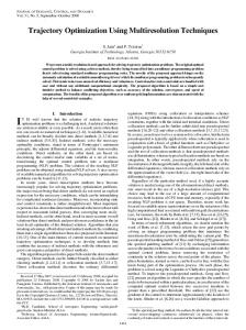
surface finish is 0.8 μm or better, and the airfoil surface tolerance is ±0.04 mm.9 Lian and Liou5 performed deterministic design optimization for this blade. Here we incorporate uncertainties into the actual design problem and evaluate its probability of failure. In engineering design, the probability of failure is usually based on the maximum stress failure criterion, which states that yielding (failure) occurs when the von Mises stress exceeds the yield strength. The blade is made of generic titanium (Ti-6V-4Al),9 whose properties are listed in Table 1. We notice that the titanium yield limit is in the range of 786–910 MPa, which is much higher than the mean response of the maximum stress, 464 MPa. There is no design violation of the structural constraint if the criterion is based on the yield stress and a safety factor of 1.5. Furthermore, the blade experiences dynamic force instead of static force. The use of yield limit makes the RBDO less meaningful. For demonstrative purposes, the resistance is chosen as the endurance limit that is the maximum stress or range of stress that can be repeated indefinitely without failure of the material. Now the failure criterion states that failure occurs when the von Mises stress exceeds the endurance limit. In our study, the von Mises stress is computed under the operating conditions. Because the blade has a very good surface finish, the impact of the randomness in shape manufacture can be tightly controlled. Therefore, we treat design variables that parameterize the blade geometry as deterministic variables. Later on, we will call them deterministic design variables. The material density can be measured with good accuracy and we treat it as deterministic. In our computation it is set as 4510 kg/m3 . The Young’s modulus is a random variable, too; however, it does not change the value of the von Mises stress, and we take its nominal value. Therefore, there are two random variables that will be factored into the RBDO: the Poisson ratio and the endurance limit. We assume that they have normal distributions around their means. Because a normal distribution, which is valid from −∞ to +∞, lacks a physical interpolation, we consider the random variable as belonging to a range bounded by its mean ±3σ . Here σ is the standard variation. In the presence of uncertainties, the maximal von Mises stress, S, and the endurance limit, R, are random variables in nature. Their randomness is characterized by their probability density functions, f S (s) and f R (r ). The schematic distribution functions of the endurance limit f R and maximum stress f S are plotted in Fig. 2.

W p02 / p01 P f (R < S) ≤ Pt |m˙ − m˙ b |/m˙ b < 0.05% d L ≤ d ≤ dU

(1)

where W is the blade weight; p02 / p01 is the stage pressure ratio; and P f is the probability of failure, which is based on the maximum stress criterion. The criterion states that failure occurs when the maximum stress S is larger than the resistance R. The variable m˙ is the compressor mass flow rate; d is the vector of design variables parameterizing the blade shape; and d L and dU are the lower and upper bounds of the design variables. The aerodynamic objective is to maximize the stage pressure ratio and the structural objective is to minimize the total structural weight. These two objectives are competing. Improving one objective will jeopardize the other. This conclusion sounds contradictory to some statements in multidisciplinary wing design, which state that a thinner wing usually gives a better aerodynamic performance than a thicker wing. These statements are usually based on the assumption that flow attaches to the wing and is considered as inviscous. We study the transonic compressor blade, which is characterized by shock–boundary interaction and flow separation. The flow inside the compressor is described by three-dimensional Navier–Stokes equations. A potential flow solver is not sufficient. In this multiobjective optimization problem, instead of having a single optimal solution that is better than all the others in terms of both objectives, our problem has a set of compromise solutions, among which no solution is better than the others in terms of both objectives. In the context of multiobjective optimization, these compromise solutions are called Pareto optimal solutions. The curve formed by joining these solutions is known as the Pareto optimal front. This optimization is performed under two constraints: the aerodynamic one is to maintain a comparable mass flow rate as the baseline; the structural one is set so that the failure probability, P f , is less than a target threshold, Pt . A new blade design is constructed by imposing a perturbation blade upon the baseline rotor67 blade. We parameterize the perturbation blade instead of the baseline. To do that, we construct perturbation airfoils at the four span locations (hub, 31%, 62%, and tip). Each airfoil is defined by a mean camber line and thickness distribution and is parameterized by a third-order B-spline curve. The thickness distribution is determined by five design variables and the camber by three. We linearly interpolate the four airfoils in the spanwise direction and obtain a perturbation blade. Therefore, we have 34 design variables in the optimization problem; among them 32 design variables, which parameterize the blade geometry, are deterministic and two variables are random.

370

LIAN AND KIM

III.

Monte Carlo Simulation

In reliability analysis, the first step is to decide on performance criteria, random parameters, and functional relationships corresponding to each performance criterion. Such a relationship can be written as Z = g(X 1 , X 2 , . . . , X n )

(2)

where Z represents the performance criterion, and X i is the random variable. The limit state is usually defined as Z = 0, which sets the boundary between safe and unsafe regions in the random variable space. If the failure event is defined as g < 0, then the probability of failure P f can be calculated as

Pf =

···

f X (x1 , x2 , . . . , xn ) dx1 dx2 . . . dxn

(3)

g 1, the probability of failure is less than the target one, and thus the design exceeds the safety requirement; if Psf = 1, the design has a probability of failure equal to the target one. Therefore, the following two expressions are mathematically equivalent: 1 − Psf ≤ 0

(9)

P f (S F ≤ 1) ≤ Pt

(10)

However, Eq. (9) is advantageous in terms of accuracy. Based on this discussion, we can use PSF in our RBDO problem and the problem can be equivalently reformulated as follows. Minimize: Maximize: Subject to:

VI.

W p02 / p01 1 − Psf ≤ 0

(11)

The constraints are kept the same as those stated in Eq. (1). It is simple and straightforward to compute the PSF using the MCS. Suppose we perform N simulation cycles using the MCS around one design point, we compute the safety factor for each cycle, and we sort the safety factor in ascending order and have the following sequence: {S F,1 , S F,2 , . . . , S F,i , . . . , S F,N },

S F,i − 1 ≤ S F,i

(12)

If the target failure probability is Pt , then the PSF has the value S F,i , where N Pt − 1 < i ≤ Pt N

V.

(13)

Reliability-Based Optimization Using Response Surface Approximation

From our previous discussion we know that the MCS requires a larger number of function evaluations to obtain a reasonably good accuracy. With a target probability of failure of 10−4 , it takes 1 million simulations to ensure percentage error less than 20%. If these computations are exclusively based on the fluid solver and structural solver, this will be extremely computationally extensive, if not impossible. It takes about 694 days to evaluate this number of cases using the structural solver on Intel Intanium processors at 1.3 Ghz. The use of approximation models is commonly practiced to reduce the computational cost. Response surface models are built to approximate computationally expensive problems, typically using low-order polynomials. The response surface model is normally chosen to be a low-order polynomial. The second-order polynomial is widely used due to its flexibility and ease of use. A second-order response surface model with d variables can be written as follows: y = β0 +

d i =1

βi xi +

d i =1

βii xi2 +

j −1 d

surface (DRS).11 The ARS is fitted to the function in terms of both deterministic variables and random variables, whereas the DRS is fitted to the function exclusively in terms of deterministic variables. In our studied problem the ARS is fitted to von Mises stress in terms of the 32 design variables and the random variable Poisson ratio. At each design point, the probabilistic sufficiency factor is computed by the MCS based on the ARS. The DRS is fitted to the probabilistic sufficiency factor in terms of the 32 deterministic design variables only. The primary purpose of the DRS is to filter the noise from Monte Carlo simulation. The objective functions and the structural constraint are also approximated with second-order response surfaces. As we will see in the next section, the use of response surface approximation also facilitates the multidisciplinary optimization.

βi j xi x j + ε

Fluid Solver and Structural Solver

A high-fidelity CFD tool, TRAF3D, is used to analyze aerodynamics of the compressor blade. TRAF3D solves three-dimensional Reynolds-averaged Navier–Stokes equations. The space discretization uses a second-order cell-centered scheme with eigenvalue scaling to weigh the artificial dissipation terms. The system of equations is advanced in time using an explicit four-stage Runge–Kutta scheme. The two-layer eddy-viscosity model of Baldwin and Lomax is used for the turbulence closure. Details about the implementation of TRAF3D and its capability can be found in the work of Arnone et al.,14 Arnone,15 and Lian and Liou.4,5 The computational grid with three blades is shown in Fig. 4. In our simulation we compute only one passage and apply periodic boundary conditions to the others. We use 0.6 × 106 nodes to model a single passage. With Intel Intanium processors at 1.3 Ghz the turnaround time is 1 h for a simulation. We model the blade with quadrilateral plate elements, which are commonly used for modeling plates, shells, and membranes. We use the commercial software ANSYS to perform static structural analysis. In each element, we assume element-constant thickness and element-constant pressure. By doing this we avoid zero-thickness elements at the leading and trailing edges. The blade is structurally fixed at the hub. Therefore, the nodes at the hub are fully constrained. Each node has three translational degrees of freedom and three rotational degrees of freedom. The multidisciplinary design optimization approach for compressor blade using high-fidelity analysis tools is presented in the work of Lian and Liou,16 where a jig-shape approach is adopted to build the compressor blade so that the structural deformation will bring

(14)

j =2 i =1

where xi is the variable, β is the unknown coefficient, and ε denotes the total error, which is the difference between the observed value y and the approximated value with the polynomial. Note from Eq. (14) that the second-order response surface model contains (d + 1)(d + 2)/2 coefficients. Consequently, the experimental design used must contain at least that many distinct design points. When deterministic analysis models such as computational fluid dynamics (CFD) tools are used, a good experimental design tends to fill the design space rather than to concentrate on the boundary. We apply the Latin hypercube sampling algorithm13 to sample the design points. This method tends to spread out the sampling points as evenly as possible by determining an optimal even spacing. Lian and Liou found that a 20–80% overdetermined design for the second-order response surface model gave reasonably good results.4 Two popular response surface models in reliability-based design are the analysis response surface (ARS) and the design response

Fig. 4

Structured grid for single passage with 6.0 × 105 nodes.

372

LIAN AND KIM

the blade to its desired shape. By doing so the structural deformation on the aerodynamic performance is corrected.17 The jig-shape approach greatly simplifies the multidisciplinary design process because now we only need to transfer the aerodynamic forces from the CFD grid to the finite element grid. The transfer of aerodynamic forces is a little bit involved because it is necessary to ensure that the interpolation is consistent and conservative. A thin plate interpolation method18 is adopted for that purpose. The thin plate interpolation is derived based on the principle of virtual work; it automatically guarantees the conservation of energy between the flow and the structural systems.19 A grid sensitivity test is also performed and a grid with 2401 elements gives a satisfactory results and is adopted. The structural system has 14,700 degrees of freedom.

VII.

tion of the failure probability. In the plot we sort the design points according to their probability of failure in ascending sequence. The probability of failure changes by several orders of magnitude over a narrow range. A quadratic response surface may not be efficient to capture the change. A high-order response surface model may be required to capture the steep variation. However, it demands more design points to fit the coefficients. In addition, we can see that more than 90% of the design has a zero failure probability. Not enough gradient information will be provided in the optimization procedure if a response surface is built based on the failure probability. Even if the reliability index is used, we still could not avoid the large portion of flat region. On the other hand, the distribution of Psf in Fig. 6 shows smooth variation. For comparison purposes we construct the DRS for both the probability of failure and probability sufficient factor. The statistical measures are shown in Table 2. We can see that the fitting of the failure probability is poor in terms of the statistical measures. However, the DRS of the probability suf2 ficient factor has good statistical measures. The values of Radj and %RMSE are 0.9994 and 0.002337, respectively.

RBDO Procedure

We summarize the procedure of the RBDO as follows: 1) Sample design points based on both deterministic design variables and random variables with Latin hypercube sampling. 2) Evaluate the design points with the high-fidelity analysis tools. 3) Construct the ARS model for the maximum stress based on both the deterministic design variables and random variables. 4) Perform Monte Carlo simulations based on the ARS to extract the probability sufficient factor. 5) Construct the DRS of the objective functions and constraints exclusively based on the deterministic design variables. 6) Perform multiobjective optimization using a real-coded genetic algorithm. 7) Improve the convergence to the Pareto-optimal front with a gradient-based method. 8) Choose representative Pareto-optimal solutions to validate against the high-fidelity tools.

VIII.

Numerical Results

In the problem described in Eq. (1) there are 32 deterministic design variables and 2 random variables. The objective functions and the aerodynamic constraint therein are only affected by the deterministic design variables, whereas the maximum stress is affected by both the deterministic design variables and one random variable, i.e., the Poisson’s ratio. The random variable, endurance limit, which is factored into the computation of probability sufficient factor, does not influence the maximum stress. Therefore, our sampling of design points is based on the 32 deterministic design variables and the random variable Poisson ratio. The ARS built for the maximum von Mises stress therefore has 33 variables and 595 unknown coefficients. With the Latin hypercube sampling we sample 1024 design points, representing a 61% overdetermined design. These design points are evaluated using the aforementioned fluid and structure solvers. The accuracy of the response surface approximation is evaluated by statistical measures, including the adjusted 2 coefficient of determination (Radj ) and the root mean square error (RMSE) predictor. The adjusted coefficient of determination is more comparable over models with different numbers of parameters by using the degrees of freedom in its computation. It measures the proportion of the variation accounted for by fitting means to each 2 factor level. Table 2 shows the test results. The value of Radj for the 2 maximal stress is 0.8369; the stage pressure rise has a value of Radj larger than 0.98 and a %RMSE close to zero, indicating that the quadratic response surface model gives accurate representations. Monte Carlo simulation is performed based on the built ARS. One million simulations are performed at each design point. At each design point we extract the probability of failure and probabilistic sufficiency factor for the 1024 designs. Figure 5 shows the distribuTable 2 Error statistics R2 2 Radj RMSE %RMSE

Fig. 5

Distribution of probability of failure of the 1024 design points.

Fig. 6 Distribution of probability sufficient failure of the 1024 design points.

Statistical measures of the quadratic response surface approximations

p02 / p01

W

m˙

SN

Psf

Pf

0.9949 0.9888 0.564 × 10−3 0.3000 × 10−3

0.9999 0.9999 0.800 × 10−5 0.1175 × 10−3

0.9979 0.9954 0.4246 × 10−2 0.1270 × 10−3

0.9262 0.8369 0.1282 × 108 0.2761 × 10−1

0.9994 0.9987 0.2637 × 10−2 0.2337 × 10−2

0.6638 0.2572 0.2851 × 10−1 0.1425 × 103

373

LIAN AND KIM

Fig. 8

Comparison of baseline with optimal solutions.

Fig. 7 Genetic algorithm convergence history and solutions from hybrid method.

Our problem described in Eq. (1) is a multiobjective optimization problem with a set of Pareto optimal solutions. To facilitate the optimization, we use a real-coded genetic algorithm. We set the population size as 320. Figure 7 shows the solutions with different generation sizes. The convergence rate at the beginning is fast, and it gradually then slows down. This phenomenon is typical for genetic algorithms, which usually suffer a low convergence rate when the optimal is approached. One remedy is to use a hybrid method. The basic idea is to switch to a gradient-based method to improve the convergence after the genetic algorithm. For that purpose we use the design optimization tools (DOT),20 which are software based on gradient-based methods. Figure 7 shows that DOT does improve convergence. To further appreciate the capability of genetic algorithms for handling multiobjective optimization, we also perform optimization exclusively based on gradient-based methods. To do that, we transform the problem in Eq. (11) into the problem that follows. Minimize: Subject to:

w1 W − w2 p02 / p01

w1 + w2 = 1.0,

w1 ≥ 0, w2 ≥ 0

(15)

Fig. 9 Comparison between the maximal pressure ratio design and the baseline at the 10% span from the hub.

(16)

We convert the multiobjective optimization problem into a singleobjective optimization problem by introducing-weight function. All the constraints are kept the same and DOT is employed as the optimizer. We notice that even though it obtains some solutions better that those from the hybrid method, the gradient-based method fails to identify some regions on the Pareto-optimal front. In addition, we notice that the gradient-based method is sensitive to the initial conditions. The solution from genetic algorithms is also affected by the initial conditions. However, the effect diminishes with the increase of generation size. We compare Pareto-optimal fronts with different initial conditions and find no evident difference after the 8000th generation. In total there are 693 Pareto optimal solutions lying on the Pareto optimal front. We choose 15 representative optimal design points from the Pareto optimal front using the K-means clustering algorithm to verify against the high-fidelity analysis tools. K-means clustering is a method that chooses a set of data points from the Pareto-optimal front to accurately represent the distribution of whole date points.4,21 The distribution of the selected data points is shown in Fig. 8. We also compare the baseline rotor67 with the optimal solutions. Clearly the optimization process decreases the blade weight and increases the stage pressure ratio as well. We show the blade difference between the baseline rotor67 and the optimal design with maximum pressure ratio. At the 10% span (Fig. 9), the maximum pressure ratio design has a larger camber but less thickness than the rotor67 design. The thinner airfoil contributes to the lighter weight of the new design. The difference in the pressure distribution is rather small. The same conclusion can be made at the


50% span (Fig. 10). At the 90% span (Fig. 11), the high-pressure ratio design has a slightly smaller camber and thinner airfoil than the rotor67.

IX.

Error Analysis

From the operation we can identify that error of the computed PSF in Fig. 5 comes from two primary sources: the approximation of maximum stress with ARS and the limit size of simulations in the MCS. Certainly there are errors associated with the fluid solver

374

LIAN AND KIM


Fig. 12 Approximation of maximum stress for one specific optimal design with quadratic response surface.

and the structural solver; however, we omit those so that we can exclusively compare the errors from the ARS and the MCS. For the studied problem with a target probability of failure of 10−4 and 1 million simulations in the MCS, the percentage error in P f associated with the MCS is 20%. In modeling the maximum stress with ARS, the %RMSE is α = 0.02761. If the maximum stress based on the ARS is S, then the actual maximum stress is estimated in the range of S(1 ± α). Here we should note that the use of RMSE% is not perfectly fitting at this circumstance because the %RMSE is calculated based on the points used to constructed the response surface model and the prediction error for new point could be larger than %RMSE. If the endurance limit takes another random value, R, and the safety factor is computed based on Eq. (6), then the actual safety factor is in the range of (R/S)[1/(1 ± α)]

(17)

Plugging α = 0.02761 into the above formulation, we can easily estimate that the uncertainty in the safety factor (also in PSF) is larger than 0.02. Hence the relative error of the probability failure associated with the ARS is 20,000%, which is much larger than the relative error associated with the MCS. Because it will be time-consuming to compute the PSF directly from the structural analysis, we use the surrogate model and the MCS to evaluate it instead. Therefore, the inaccuracy arise from three sources: the ARS approximation, the DRS approximation, and the limit size of the MCS. We further validate the PSF for each representative optimal design. From our previous discussion we know that we can compute the PSF using the MCS. By doing this we need to evaluate the safety factor R/S using the MCS at the optimal design point. The value of the endurance R can be directly obtained based on the distribution function. For a fixed blade shape, the maximal stress S for a specific design is only a function of the Poisson ratio. Our discussion indicates that with a target probability of failure of 10−4 we need one million simulations to ensure that the relative error of the failure probability is less than 20%. Even though the structural analysis is relatively cheaper than the computational fluid dynamics analysis, it is computationally formidable to perform that many simulations exclusively based on structural analysis. On the other hand, conventional wisdom tells us that it is not a sound idea, either, to evaluate the PSF by using the previously constructed ARS model for the maximum stress. What we do here is to construct a new response surface model to approximate the response of the maximal stress to the Possion’s ratio at one selected optimal design point. At each design points we uniformly sample 21 points for the Poisson’s ratio. These design points are then evaluated with the structural solver. Our statistical analysis shows that the second-order response surface gives an accurate representation of the relationship between

Fig. 13 Verified probability sufficient factor at the optimal design and from the DRS prediction. 2 the Poisson’s ratio and the maximum stress. The value of Radj is 1.00 and the %RMSE is 4 × 10−6 . Based on Eq. (17) we can compute the actual range of the PSF. A representative quadratic fitting and the sampled points are shown in Fig. 12. The optimal design is then substituted into the newly constructed response surface to evaluate its PSF using the MCS. This calculated PSF is compared with the predicted values in the optimization process. The comparison is illustrated in Fig. 13. We further adjust the PSF value based on Eq. (17). All the PSF are larger than 1.0, indicating that the safety is beyond our target. We also want to compare the results from the reliability design and the deterministic design. It is difficult to find the relationship between the PSF in RBDO and the nominal safety factor in the deterministic design and it is difficult to transform the RBDO into an equivalent deterministic design problem. Therefore, this comparison is for demonstration purposes only. In deterministic design, the material properties are taken as their mean values with the Poisson ratio of 0.34 and endurance limit of 547.5 MPa, respectively. The structural constraint in Eq. (11) is replaced with the following expression:

S F > S B,F

(18)

where S B,F is the baseline safety factor of 1.18. The optimization procedure, which shares many similarities with the RBDO procedure reported in this paper, performs optimization based on surrogate models and a hybridized optimizer. The details are outlined in

375

LIAN AND KIM

We identify the sources of numerical errors in the reliability-based design optimization. In addition, we further quantify the numerical errors. We realized that further research was required in evaluating the accuracy of the response surfaces, related to sampling, regression, and modeling, which is beyond the scope of this paper.

Acknowledgment The authors thank Raphael T. Haftka at the University of Florida for his insightful comments.

References 1 Oyama, A., Liou, M. S., and Obayashi, S., “Transonic Axial-Flow Blade

Fig. 14 Verified probability sufficient factor at the optimal design from deterministic design optimization.

the work of Lian and Liou.5 The preselected 1024 design points are used to build the quadratic response surfaces. Likewise, we choose 14 optimal design points from the resulting Pareto-optimal front to verify against the high-fidelity analysis tools. At each optimal point we assume that the material properties follow the same normal distributions as used in the RBDO. Its PSF with a probability of failure less than 10−4 is computed with the same procedure utilized in the RBDO. The PSF distribution is plotted in Fig. 14. We notice that some designs have a PSF value less than 1.00, indicating that the safety requirement is not met. In addition to the statistical test for the accuracy of response surfaces in Table 2, we compared the actual performance values with those from the response surfaces at the representative optimal points. It turns out that all performance values show reasonably accurate approximation with a relative error within 5% using the response surfaces, except for the maximum stress, which has a relative error as large as 10%. Such a discrepancy has not been reported before in the literature. Possible explanations are as follows: 1) Maximum stress is a local variable, whereas other objectives and constraints are global. It is difficult to capture the local phenomenon using a global description such as the response surface method. 2) The maximum stress performance is not a differentiable function of the deterministic design variables/random variables because it employs the noncontinuous function max, which also is not a differentiable function. 3) The statistical measures reported here, which are used to measure the amount of reduction in the variability of response functions obtained using the sample designs in the model, do not warrant good predictions of new values.

X.

Conclusions

In this paper, we demonstrated a reliability-based design optimization technique when both aerodynamic and structural performances were considered. The design uncertainty came from the material properties. Our objectives were to maximize the stage pressure ratio and to minimize the blade weight. A second-order response surface model was built to make it possible to perform such a computationally intensive analysis and optimization process. A genetic algorithm was used to facilitate the multiobjective characteristics of our problem. The reliability analysis was performed based on Monte Carlo simulation. To address the accuracy problem resulting from using probability of failure in regions of low probability of failure, the probabilistic sufficient factor was adopted. Our numerical results showed that we could achieve a new design with lighter weight, higher pressure ratio, and more reliable performance than the baseline rotor67.

Shape Optimization Using Evolutionary Algorithm and Three-Dimensional Navier–Stokes Solver,” Journal of Propulsion and Power, Vol. 20, No. 4, 2004, pp. 612–619. 2 Benini, E., “Three-Dimensional Multi-Objective Design Optimization of a Transonic Compressor Rotor,” Journal of Propulsion and Power, Vol. 20, No. 4, 2004, pp. 559–565. 3 Mengistu, T., and Ghaly, W., “Single and Multipoint Shape Optimization of Gas Turbine Blade Cascades,” AIAA Paper 2004-4446, Aug.–Sept. 2004. 4 Lian, Y., and Liou, M. S., “Multiobjective Optimization Using Coupled Response Surface Model and Evolutionary Algorithm,” AIAA Journal, Vol. 43, No. 6, 2005, pp. 1316–1325; also AIAA Paper 2004-4323, 2004. 5 Lian, Y., and Liou, M. S., “Multiobjective Optimization of a Transonic Compressor Rotor Using Evolutionary Algorithm,” Journal of Propulsion and Power, Vol. 21, No. 6, 2005, pp. 979–987; also AIAA Paper 2005-1816, 2005. 6 Enevoldsen, I., and Sorensen, J. D., “Reliability-Based Optimization in Structural Engineering,” Structural Safety, Vol. 15, No. 3, 1994, pp. 169–196. 7 Tu, J., Choi, K. K., and Park, Y. H., “A New Study on Reliability-Based Design Optimization,” Journal of Mechanical Design, Vol. 121, No. 4, 1999, pp. 557–564. 8 Qu, X., Haftka, R., Venkataraman, S., and Johnson, T., “Deterministic and Raliability-Based Optimization of Composite Laminates for Cryonenic Enviroments,” AIAA Journal, Vol. 41, No. 10, 2003, pp. 2029–2036. 9 Strazisar, A. J., Wood, J. R., Hathaway, M. D., and Suder, K. L., “Laser Anemometer Measurements in a Transonic Axial-Flow Fan Rotor,” NASA TP 2879, 1989. 10 Haldar, A., and Mahadevan, S., Probability, Reliability and Statistical Methods in Engineering Design, Wiley, New York, 2000. 11 Qu, X., and Haftka, R., “Reliability-Based Design Optimization Using Probabilistic Factor,” Journal of Structural and Multidisciplinary Optimization, Vol. 27, No. 5, 2004, pp. 302–313. 12 Birger, I. A., Safety Factors and Diagnostics: Problems of Mechanics of Solid Bodies, Sudostroenve, Leningrad, 1970, pp. 71–82 (in Russian). 13 Beachkofski, B., and Grandhi, R., “Improved Distributed Hypercube Sampling,” AIAA Paper 2002-1274, 2002. 14 Arnone, A., Liou, M. S., and Povinelli, L. A., “Multigrid Calculation of Three-Dimensional Viscous Cascade Flows,” NASA TM-105257, 1991. 15 Arnone, A., “Viscous Analysis of Three-Dimensional Rotor Flow Using a Multigrid Method,” Journal of Turbomachinery, Vol. 116, No. 3, 1994, pp. 435–445. 16 Lian, Y., and Liou, M. S., “Aero-Structural Optimization of a Transonic Compressor Blade,” Journal of Propulsion and Power (to be published); also AIAA Paper 2005-3634, 2005. 17 Sobieszczanski-Sobieski, J., and Haftka, R. T., “Multidisplinary Aerospace Design Optimization: Survey of Recent Development,” Structural Optimiation, Vol. 14, No. 1, 1997, pp. 1–23. 18 Duchon, J. P., “Splines Minimizing Rotation-Invariant Semi-Norms in Sobolev Spaces,” Constructive Theory of Functions of Several Variables, Oberwolfach 1976, edited by W. Schempp and K. Zeller, Springer-Verlag, Berlin, 1977, pp. 85–100. 19 Liu, F., Cai, J., Zhu, Y., Tsai, H. M., and Wong, A. S. F., “Calculation of Wing Flutter by a Coupled Fluid-Structure Method,” Journal of Aircraft, Vol. 38, No. 2, 2001, pp. 334–342. 20 DOT User’s Manual, Version 4.20, Vanderplaats Research and Development, Inc., Colorado Springs, CO, 1995. 21 Bishop, C. M., Neural Network for Pattern Recognition, Oxford Univ. Press, 2003.

E. Livne Associate Editor