Exact solutions have been found for the existence and stability of limit cycles, allowing meaningful ..... li'mit) including higher modes does produce a stable motion for long times. ... This aspect of the general problem is not fully understood.
REMARKS ON THE TWO-MODE APPROXIMATION TO THE NONLINEAR BEHAVIOR OF PRESSURE OSCll.LATIONS IN COMBUSTION CHAMBERS· F. E. C. Culick California Institute of Technology L. Paparizos Carnegie Mellon University ABSTRACT This paper summarizes recent work on the approximation to nonlinear pressure oscillations using two modes. A large part of the effort has been concerned with the consequences of gasdynamic nonlinearities of second order in the fluctuations. It appears that the two-mode approximation is valid over a broad range of the linear parameters that govern the global qualitative behavior, particularly if the lower mode is the unstable mode. Exact solutions have been found for the existence and stability of limit cycles, allowing meaningful comparison with numerical solutions obtained with larger numbers of modes considered. The nonlinear analysis to second order does not contain "triggering" - nonlinear instability of a linearly stable system - because the nonlinear processes order terms involving the mean flow speed, or DC shifts in the amplitudes of oscillation do produce triggering. 1. INTRODUCTION
There are two strategies for investigating thoretically the problem of combustion instabilities: numerical analysis based the partial differential equations of conservation; or some sort of approximate analysis founded on reduced forms of the partial differential equations. A fully developed theory of the phenomena must involve both sorts of activities. In this paper we are concerned with a particularly useful form of approximate analysis constructed with a system of ordinary differential equations produced by spacial and time averaging of the partial differential equations. It is well to remark first that numerical analysis of the partial differential equations is a fundamentally important part of the theoretical work. Because formal mathematical methods are several limited, numerical methods offer the only means of obtaining quantitative results for problems accurately modeling the physical circumstances existing in real problems. Work of this sort, which to-date has been limited to two-dimensional, axisymmetrical or, in most cases one-dimensional problems, constitutes essentially the application of computational fluid dynamics to internal flows. Even with the approximations inherent in modeling some of the processes (mainly combustion and turbulent flow), and the obvious characteristic that each numerical computation applies to a single well-defined problem, the results provide the only standard against which the accuracy of approximate solutions can be measured. Thus numerical analysis will in principle fulfill two needs: accurate simulations of complex internal flows, potentially a useful contribution in later stages of design and development; and checks of approximate results. Approximate analysis likewise has two primary functions: to provide deeper understanding of the general behavior; and as a basis for less expensive computational methods usable in routine fashion and therefore available for preliminary design work and investigation of trends of behavior, such as parametric studies. Because numerical analysis provides results for a relatively small number of special cases, it is both expensive and time consuming to perceive reasons for the particular behavior found and to extract useful guidelines, "rules of thumb". Moreover, even with the recent advances in computational resources, numerical calculations of the sort required for internal flows are still expensive and restricted. We have therefore concentrated on developing an approximate analysis to fill the requirements both for basic theoretical work and for convenient routine analysis of actual problems. Another important feature is that the formal results not only provide useful guidelines for design work but also serve as a framework for planning experiments and interpreting test results. • This work was supported by Caltech fund. and by the Office of Naval Research, Contract N00014-84-K--{)434. Approved for public release; distribution is unlimited.
The approximate analysis used here is based on a form of Galerkin's method and, in most of our work, time averaging as well. As a result, most of the calculations are based on systems of coupled nonlinear first order differential equations. This approach provides a convenient point of view for studying combustion instabilities and sets the mathematical developments squarely in the context of the contemporary theory of nonlinear dynamical systems. Use of Galerkin's method to study combustion instabilities was first made by Zinn and Powell (1968, 1970) for liquid rockets and by Culick (1971, 1975, 1976) for solid rockets. The analysis described here is based largely on the last work, Culick (1976), in which the method of averaging was introduced. Because the derivation of the system of equations has been given in several places, we shall not repeat the process here, but rather concentrate on the specialization to two modes, for longitudinal oscillations. Galerkin's method produces a system of second order ordinary differential equations representing the time evolution of an infinite set of coupled nonlinear oscillators. One oscillator is associated with each classical acoustic mode; the second order equation is for the amplitude of the mode, i.e. of the oscillator's motion. Timeaveraging replaces the second order equation by two first order equations. Hence if N modes are considered, one has to solve 2N first order equations. The linear behavior of each mode is characterized by two parameters, the growth constant and the frequency shift, both due to the various perturbations of the classical acoustics prevailing in the absence of combustion and mean flow. Nonlinear gasdynamics introduces no new parameters, so if no other nonlinear processes are accounted for, both the linear and nonlinear behavior are determined by the values of the linear parameters, 2N for N modes. . Numerical solutions to the set of equations is inexpensive and easy to achieve. The point here is to investigate the formal behavior and for that purpose it is necessary to truncate the system to two modes, i.e. four equations. It happens that if gasdynamics is the only nonlinear process included, and only second order nonlinearities are allowed, the four equations can be reduced to three by a simple transformation. That simplification is the basis for the theoretical work described here. 2. FORMULATION OF THE TWO-MODE APPROXIMATION After the dependent variables are expressed as sums of mean and fluctuating parts, a nonlinear wave equation can be formed for the pressure, with its boundary condition: V'2
I _
P
..!.. _ 8 2 p' = h 8t2
(i2
n· V'p' =-1
(2.1) (2.2)
The pressure and velocity fluctuations are then expanded in the normal modes tP,..(Tj with time-varying amplitudes '7,..(t):
p'
= 15 L '7,..(t)tP,..(Tj
L
iii =
~7],..(t)V'tP,..(Tj ,k,..
(2.3)
(2.4)
Now multiply (2.1) by tPm, substitute (2.3) for pi and integrate over volume. After use of the boundary condition (2.2), some manipulations give the equation for '7,..: d
2
'7,..
dt 2
2
+ W,..'7,..
= F,..
where the force is the spacial average of the functions k and
(2.5)
I: (2.6)
For many practical situations, the amplitudes are oscillatory with slowly varying amplitudes and phases. Thus we assume that a good approximation for '7,.. is
(2.7) This equation really serves to define the function An(t) and B,..(t). Time averaging eventually leads to the equations for An and Bn:
J
',
t+r
dA,.. -d-
t
-1-
==
W,..T
F,..cosw,..t dt
t
(2.8)a, b
where T is the interval of averaging. The case of longitudinal modes, for which w,.. == nW1, is special. The integrands in (2.8)a,b are then periodic and the range of integration can be shifted from (t, t + r) to (0, r). Then if only gasdynamic nonlinearities to second order are accounted for, the equations can be written dAn
-;It ==
nf3
a,..A,..
,..-1
+ OnBn + 2"" L
(A.A n _. - B.Bn _.)
i=1 00
- nf3 L(An+.A.
+ Bn+.B.)
.=1
(2.9)a, b
00
+ nf3L(An+.B. - Bn+.A.)
.=1 These are slightly re-arranged but equivalent forms of the corresponding equations given in Culick (1976) and used in many works since. The quantity f3 shown explictly here can be absorbed as a time scale, so it is not a true parameter: f3
+1 = ('--)W1 8,
(2.10)
For the case of two modes, the form governing equations can be transformed to the following set of three [Paparizos and Culick (1988a)]: dYl dt = ( a1 +Y2 ) Y1 dY2 = a2Y2 + I" dt u2 dY3 dt = -1 02 -
201IY3
20 1 lY2
+ 2Y3 2 -
+ a2Y3 -
Yl 2
(2.11)a, b, c
2Y2Y3
where Y1
= f3r1
Y2
= f3r2 sin(tP2 -
Y3
=
2tPd
(2.12)a, b, c
102 - 20 1 1 (0 _ 20df3r2cos(tP2 - 2tPd 2
(A,.. 2 + f3,.. 2) l and tan tP,..
where r,.. = = A,.. I B,... These equations can be solved exactly and therefore provide complete information about the behavior of a two-mode system, when only second order gasdynamical nonlinearities are considered. The results are significant not only for their own sake as an exact solution for a special case, but also because they form a convenient basis from which the analysis can be extended to cover other perturbations, including third order terms and stochastic sources, for example.
3. EXISTENCE AND STABILITY OF PERIODIC SOLUTIONS (LIMIT CYCLES) Besides reducing the number of equations by one (possible because the zero phase of the oscillations in the limit cycle can be freely chosen), the transformation (2.12)a,b,c also maps periodic solutions of the equations for (AI, A 2 , B 1 , B 2 ) into fixed points of equations (2.11)a,b,c. That is, limit cycles of the original system are determined in the variable (Yt, Y2, Y3) by setting dy ... ldt = o. With lin = 0, equations (2.11)a,b,c have two solutions for the fixed points; the trivial one for which y/' = 0, and
(3.1 )a, b, c p 0:1(0 2 - 20d Y3 = - --'------'0:2 + 20:1
It follows from (3.1)a that the condition for existence (YI must be real) is (3.2) This reflects the physical attribute that in the limit cycle, because the energy in the oscillation is constant, one mode must be unstable (0: > 0) and the other unstable (0: < 0). Note that the case 0:10:2 > 0 implies that both modes are either unstable or both are stable. The first condition implies that the energy of the system increases without limit, an unstable motion; the second condition characterizes the trivial "limit cycle," the state of no motion. Local stability of the limit cycle is obtained by investigating small motions about the motion represented by the fixed point (3.1)a,b,c. The Routh-Hurwitz criteria for stability give the three conditions:
0:1(2
+ 0:2 ) < 0
2 0:1(0: 0:1
(3.3)a,b,c
0:1
XI)
(0: 2 0:1
X2) > 0
where
(Po - 1) ± ../(Po - 1) (3Po 1 + Po
+ 1)
(3.4)
and (3.5) The condition (3.2) for existence shows that there are two cases to consider: (0:1 > 0, 0:2 < 0), for which the first mode is unstable; and (0:1 < 0, 0:2 > 0), when the second mode is unstable. Figure 1 shows the ranges of the parameters in which the oscillations for these two cases are stable. Note that the coordinates are Po and 0:2/0:1; in contrast to the results found by Awad and Culick (1985), here we have found the conditions covering all values of the linear parameters. It is important to recognize that the two cases (0:1 > 0, 0:2 < 0) and (0:1 < 0, 0:2 > 0) exhibit substantially different physical behavior because the gasdynamic nonlinearities tend naturally to cause energy to flow upward in the spectrum. 0:1 > 0, 0:2 < 0 For this case, the inequality (3.3)b gives
(3.6) Irrespective of the values of 0 1, O2 , this condition must be met if a disturbance is to evolve into a stable periodic limiting motion. Figure 2 shows trajectories in the (YI, Y2, Y3) plane, each trajectory characterized by different initial conditions. Note that for all initial conditions, the motion is the same in the limit cycle, represented by the point P whose location is a function of 0:1, 0:2, 01 and O2 • As the values of the linear parameters are changed, P traces a line in the space, called the "center manifold" in the theory of dynamical systems. The equation for the manifold is found by setting Y2 = Y3 = 0 in (2.11)b,c. From (2.11)c, one has
(3.7) and substitution in (2.11)b leads to a third order polynomial Y2(yIl. Hence the curve is readily computed. On One may then show that a unique stable solution exists for Y2 > 0:2/2. Figure 3 shows the projection of the center manifold in the (Y2, y:d plane. (Note that 0:2/2 < 0 for the conditions assumed here).
a1
> 0,
a2
4, so these third order are numerically more significant than those arising directly with third order gas dynamic nonlinearities.
7. THE INFLUENCE OF MEAN VELOCITY ON TRIGGERING Initially in the approximate analysis described here, we deal with an expansion in two small parameters, one (denoted JL) measuring the Mach number of the mean flow field, and the other (f) measuring the amplitude of the oscillations. The ordering of terms in the equations is such that classical linear acoustics is of order f, those defining linear stability are of order JLl, second order acoustics contributions are of order l~ and so forth. Here we consider for the first time contributions that depend on the mean flow and are nonlinear in the fluctuations. We assume a mean flow field varying linearly along the axis of the chamber, il = aMN(z/ L) where MN is the Mach number at the entrance to the nozzle. Retaining terms of order JLl 2 , we eventually find the equations for l!h, Y2, Y3): dYI
dt dY2 dt
= (al
= a2Y2
dY3 + dt
(0 2
+ Y2)Yl
- 7JLY1Y3
) '). + (20 - 20 1 Y3 + 2Y3 -
201 ) Y2
+ a2Y3 -
Yl 2
2Y2YS
+ 14101Y2Y3
+ JLYI 2 -
(7.1)a,b,c
14JLY2 ').
where
For small v, the solutions for the limit cycle are (Yll')2
=-
a~ [(Y21')').
al
+ (Y31')2] (1 + 6..!!... Y31') al
+ 7JLY31' " 1 al( 14a l + (2) Y3 = - ad 02 - Otl + JL --'-'----'---'-'a2 + 2al a2 + 2al "2 a2 + 2al Y3 = --'--:-:--'=' Y21' r
r
=-
al
(7.2)a, b, c, d
•
•
12101
The solution (7.2)a,b,c represents a perturbation of the result found for second order acoustics. The second possibility, with Y31'·2 given by (7.2)d is new and particularly interesting because it contains triggering. However, as in all cases found above, triggering leads to an unstable motion, not a stable limit cycle. REFERENCES Awad, E. and Culick, F. E. C. (1985) "On the Existence and Stability of Limit Cycles for Longitudinal Acoustic Modes in a Combustion Chamber," Combustion Science and Technology, Vol. 96, pp. 195-222. Culick, F. E. C. (1971) "Nonlinear Growth and Limiting Amplitude of Acoustic Oscillations in Combustion Chambers," Combustion Science and Technology, Vol. 3, pp. 1-16. Culick, F. E. C. (1975) "Stability of Three-Dimensional Motions in a Combustion Chamber," Combustion Science and Technology, Vol. 10, pp. 109-124. Culick, F. E. C. (1976) "Nonlinear Behavior of Acoustic Waves in Combustion Chambers," Parts I and II, Acta Astronautica, Vol. 3, pp. 714-757. Paparizos, 1. and Culick, F. E. C. (1988a) "The Two-Mode Approximation to Nonlinear Acoustics in Combustion Chambers: I. Exact Solution for Second Order Acoustics," To appear in Combustion Science and Technology. Paparizos, L. and Culick, F. E. C. (1988b) "The Two-Mode Approximation to Nonlinear Acoustics in Combustion Chambers: II. Influence of Third Order Acoustics and Mean Flow in Triggering," In preparation. Yang, V., Kim, S. I. and Culick, F. E. C. (1987) "Third Order Nonlinear Acoustic Waves and Triggering of Pressure Oscillations in Combustion Chambers, Part I: Longitudinal Modes," AlA A Paper No. 87-1873. Yang, V., Kim, S. I. and Culick, F. E. C. (1988) "Third Order Nonlinear Acoustic Waves and Triggering of Pressure Oscillations in Combustion Chambers, Part II: Transverse Modes," In preparation. Zinn, B. T. and Powell, E. A. (1968) "Application of the Galerkin Method in the Solution of Combustion Instability Problems," Proceedings, XIX Congress, International Astronautical Federation. Zinn, B. T. and Powell, E. A. (1970) "Nonlinear Combustion Instability in Liquid-Propellant Rocket Engines," Thirteenth Symposium (International) on Combustion, The Combustion Institute, pp. 491-503.