A predictive map does not represent geological truth but rather a best estimate of what that area may represent on ... or interpretation) is that various enhanced images can be displayed quickly to facilitate .... CSA - Cdn$300/ scene. Magnetic ...
20 Remote Predictive Mapping: An Approach for the Geological Mapping of Canada’s Arctic J. R. Harris, E. Schetselaar and P. Behnia
Geological Survey of Canada, Ottawa Canada
1. Introduction Due to its vast territory and world-class mineral and energy potential, efficient methods are required for upgrading the geoscience knowledge base of Canada’s North. An important part of this endeavour involves updating geological map coverage. In the past, the coverage and publication of traditional geological maps of a limited region demanded multiple years of fieldwork. Presently more efficient approaches for mapping larger regions within shorter time spans are required. As a result, an approach termed Remote Predictive Mapping (RPM) has been implemented since 2004 in pilot projects by the Geological Survey of Canada. This project falls under the larger Geo-mapping for Energy and Minerals (GEM) program initiated by Natural Resources Canada. Remote predictive mapping comprises the compilation and interpretation (visual or computer-assisted) of a variety of geoscience data to produce predictive maps containing structural, lithological, geophysical, and surficial information to support field mapping. Predictive geological maps may be iteratively revised and upgraded to publishable geological maps on the basis of evolving insight by repeatedly integrating newly acquired field and laboratory data in the interpretation process. The predictive map(s) can also serve as a first-order geological map in areas where field mapping is not feasible or in areas that are poorly mapped. The fundamental difference between RPM and traditional ground-based mapping is that in the latter, the compilation of units away from field control (current and legacy field observations) is largely based on geological inference while in RPM this geological inference is repeatedly tested and calibrated against remote sensing imagery. Remote predictive mapping is of course not an entirely new philosophy for geological mapping. Geologists have long assembled diverse layers (primarily aerial photographs and aeromagnetic contour maps) of geoscience data to study the relationships between the spatial patterns for resource exploration and mapping endeavours. In the past this has been accomplished using an ‘analog’ approach, forcing maps printed on mylar to be portrayed on a uniform map scale on a light table. However, with the increasing availability of digital data sets and the routine use of geographic information systems (GIS), the task of studying relationships between data and producing innovative maps to assist field mapping has become easier and more versatile. Contrary to the ‘light table’ approach, GIS allow maps and image data to be combined, overlaid, and manipulated at any scale with any combination of layers and subjected to any integrated enhancement.
496
Earth Sciences
A predictive map does not represent geological truth but rather a best estimate of what that area may represent on the ground based on the signatures derived from the interpreted data (geophysical, geochemical, remotely sensed). For that matter, even a traditionally produced geological map may not represent the geological truth, as all maps, no matter how they are produced, may contain spatial and classification errors. Thus, geological features of a predictive map do not necessarily correspond to how these features would be classified on the ground by a field geologist. At the categorization level, the geological term attached to a unit or structural feature may even prove to be wrong; yet at the detection level, the identified feature may correspond to a hitherto unrecognized mappable unit or structure that can be targeted for follow-up fieldwork. The amount, variety, and quality of data used are obviously key factors in how closely the predictive map matches the geological patterns obtained by field mapping. Another factor is the nature of the geological terrain being mapped as the data sets and associated processing and enhancement techniques being employed will vary depending on the bedrock, surficial, and topographic environment. A remote predictive map can assist the geologist in a number of ways: (1) by predicting map units that would tentatively be assigned to rock types and/or geological formations (bedrock and surficial). This is based on establishing critical relationships between imaged physical properties (magnetic intensity, gravity, gamma-ray spectrometry, spectral reflectance, radar backscatter) and patterns obtained from available geological maps and field data, (2) by predicting areas that appear to be characterized on remotely sensed images by more complex and spatially heterogeneous geological patterns, thus focusing and prioritizing field work in these areas; likewise, areas with more homogenous signatures and simpler patterns can also be identified as possibly requiring less field work to geologically calibrate, (3) by predicting a variety of structures (foliation traces, faults, dykes, lineaments, glacial flow directions, etc.). The structural information can be used in advance of field work, to supplement field observations or as stand-alone geological information and, (4) by predicting the distribution of bedrock outcrop and other physiographic features such as wetlands, areas of forest fire burns, vegetation cover, and infrastructure to support fieldwork planning. Predictive maps can also result in a different paradigm for planning field traverses. Instead of regularly spaced traverse lines, more detailed traverses can be set up that are focused on more complex areas and on areas where bedrock outcrop has been identified. This is especially advantageous in Northern mapping campaigns where the territory is vast and mapping expenses are high. The mechanics of producing interpretations from various geoscience data sets can be greatly facilitated by GIS and image analysis technology. For example, image interpretation can be accomplished directly on a computer touch –sensitive screen as opposed to interpreting on mylar overlays. The advantage of this screen digitization process (i.e. heads-up digitization or interpretation) is that various enhanced images can be displayed quickly to facilitate interpretation by virtually real-time comparison between different data types at any scale. Multiple iterations can be undertaken and each digital interpretation can be stored as a different GIS layer. This by-passes the cumbersome procedure of scanning and digitizing hard-copy interpretations followed by georeferencing, which can introduce spatial errors. Similar to field mapping, the successful recognition and extraction of geological information is a learning process based on experience in interpreting image data in a variety of physiographic and geological settings.
Remote Predictive Mapping: An Approach for the Geological Mapping of Canada’s Arctic
497
2. RPM approach Remote predictive mapping involves the acquisition, processing, and geological interpretation of available remotely sensed data sets as well as legacy geological data. The results are predictive maps (or GIS layers) of interpreted bedrock and surficial units as well as geologic structures. Remote Predictive Mapping can be either completed in isolation from field-based mapping or can be intimately integrated with it in order to ground truth the interpretation as field mapping proceeds. Figure 1 shows a summary of the RPM
Fig. 1. Flow chart showing how RPM methods can be integrated in a geological mapping project. The grey area represents traditional field mapping methods whereas the white area represents remote predictive mapping methods. Predictive maps can be produced by enhancing and fusing various remotely sensed data and visually extracting geologic information from these products. Alternatively, a computer can be employed to automatically produce a predictive map (unsupervised approach) or by utilizing the geologist’s expertise in concert with computer analysis (supervised approach). The geological interpretations are constrained or ‘trained’ by existing geological field data and existing geological maps. The arrow that loops back from Updated Geological Maps to Enhanced and Derivative Data emphasizes that the interpretation and map compilation process can be integrated over multiple iterations of field mapping.
498
Earth Sciences
process integrated into the work flow of a geological mapping project. The shaded portion represents the activities common to the traditional geological mapping process, whereas the portion that is not shaded represents the additional activities of the RPM approach. Regardless of whether the interpretation of remotely sensed data is fully integrated into a geological mapping project or not, the following provides a systematic outline of RPM work flow. 2.1 Mapping objectives The first step in a RPM project is to define the mapping context, which includes the following: mapping focus (bedrock, surficial), nature of the geological terrain, surficial conditions and degree of exposure, physiography, data availability, quantity, and quality. These factors will determine the data that will be most useful for bedrock mapping. Bedrock mapping projects that are planned in well exposed terrain and have thin residual till cover will benefit from the integration of magnetic, gamma-ray spectrometry, optical, and radar image data. In areas where sparse outcrops alternate with thick overburden, bedrock mapping will primarily profit from the interpretation of magnetic data. In surficial mapping, optical and radar remote sensing techniques, together with gammaray spectrometry and digital terrain data, will contribute to distinguishing various types of surficial materials, identifying and mapping geomorphic features, and mapping streamlined glacial landforms that provide information on glacial movement. Geological setting and physiography of the terrain in combination with the spatial and spectral resolution, penetration depth, season of image acquisition, and aerial coverage of the remote sensing system (including airborne geophysics) are all important factors when choosing data sets for geological interpretation. 2.2 Data selection Governments and private-sector contractors and/or vendors now provide much of the geoscience data in digital format that increasingly can be accessed through the internet. The core data types that are generally acquired and interpreted for RPM projects are listed in Table 1 along with references to a sample list of websites to obtain them. In Canada, most of these data sets cover the complete landmass with the exception of gamma-ray spectrometry data. Nonproprietary, medium to low-resolution geophysical data, including magnetic and gamma-ray data were obtained from the Geological Survey of Canada’s Geophysical Data Centre. LANDSAT 7 enhanced thematic mapper scenes of 180 x 180 km optical remotely sensed data with one 60 metre resolution thermal band, six 30 metre multispectral bands in the visible to mid-infrared range, and one 15 metre panchromatic band in the visible range can be obtained, free of charge, from the Geogratis website (http://www.geobase.ca). Radarsat data is obtained from the Canadian Space Agency (CSA). Digital elevation data (DEM) (CDED at 1:50,000 and/or 1:250,000 scale) can be downloaded from the Canadian Council on Geomatics (CCOG) website (http://www.geobase.ca). The internet providers of optical remotely sensed data often include a quick-look download service that allows for the inspection of cloud cover of the scenes before downloading.
Remote Predictive Mapping: An Approach for the Geological Mapping of Canada’s Arctic
499
Data
Data provider
Cost
LANDSAT TM
Geogratis web-site http://geogratis.cgdi.gc.ca/ MDA Geospatial Services
Free to download from Geogratis Cdn$720 per scene from MDA
RADARSAT
Geogratis web-site (100m pixel mosaic of Canada) MDA Geospatial Services (http://www.rsi.ca/)– for individual scenes from the archive or acquire new data – commercial users Canadian Space Agency (CSA) – as above – for government users
mosaic –free to download MDA - Cdn$3,000 – 4,000 /scene CSA - Cdn$300/ scene
Magnetic data
Geophysical Data center (GSC) http:// gdcinfo.agg.nrcan.gc.ca
Free to download
Gamma-ray spectrometry data
Geophysical data centre http:// gdcinfo.agg.nrcan.gc.ca
Free to download
DEM – CDED
Geobase http://www.geobase.ca/
Free to download
ASTER
USGS (http://edcdaac.usgs.gov/main.asp) Information can be found at: http://asterweb.jpl.nasa.gov/ http://asterweb.jpl.nasa.gov/gallery.asp
$40.0 US per scene
SPOT
IUNCTUS Geomatics Corp. http://www.terraengine.com/
$1200.0 per scene for SPOT 4 $1.00 - $6.00 per sq km – SPOT 5
IKONOS
MDA Geospatial Services (http://www.rsi.ca/) Information can be found at: http://www.infoterraglobal.com/ikonos.htm http://www.satimagingcorp.com/galleryikonos.html
$15.0 -$30.0 per sq km
QIUCKBIRD
MDA Geospatial Services (http://www.rsi.ca/) Information can be found at: http://www.satimagingcorp.com/galleryquickbird.html http://www.ballaerospace.com/quickbird.html
See MDA web-site
ENVISAT
MDA Geospatial Services (http://www.rsi.ca/)
See MDA web-site
RESOURCESAT
MDA Geospatial Services (http://www.rsi.ca/)
$2750.0 per scene
IRS
MDA Geospatial Services (http://www.rsi.ca/)
$900.0 - $2,500.0
ERS-1 Radar
MDA Geospatial Services (http://www.rsi.ca/)
$660.0 per scene
Airborne hyperspectral data
- selected coverage of PROBE data – Baffin Island, Sudbury - Canada Centre for Remote Sensing (CCRS) and Geological Survey of Canada – Geophysical Data Centre
Selected scenes free to download
Table 1. Data sets used for the RPM projects discussed in this paper There are also a number of other specialized remote sensing systems included in Table 1 that do not yet provide complete coverage of the Canadian landmass. Optical sensors, including ASTER, SPOT, IKONOS, QUICKBIRD, WORLDVIEW I and II and airborne hyperspectral, can
500
Earth Sciences
provide a wealth of geological information but these data are not available for all of Canada. However, these data can be acquired and when available their use should be considered, since they offer imagery with either higher spectral resolution (ASTER, 14 spectral bands) or higher spatial resolution (SPOT 5, IKONOS, QUICKBIRD, WORLDVIEW). The higher spatial resolution of the latter sensor systems with 4.0 to 2.4 metre multispectral and 1.0 to 0.4 metre panchromatic data acquisition is not only useful for mapping and logistical planning but also as a navigational guide in hand-held field computers. Existing field and laboratory data and published geological maps can be integrated into the RPM process to guide, calibrate, and test interpretations (see Case Studies 5 and 9 in Harris, 2008 and Schetselaar et al., 2000). This can be accomplished by overlaying the field observations (lithological unit, strike and dip measurements) on the predictive map(s) in a GIS environment to calibrate the interpretation of geological units and structures. Field data can also be used in training computer classification algorithms. The statistical relationships between the numerical values of image data (representing spectral reflectance, magnetic field intensity, radar backscatter, etc) and lithological units can be computed at field stations and then used to predict other areas with similar signatures. Geological mapping is increasingly being supported by digital field-data capture technology using hand-held computers and global positioning systems (GPS). This is a revolutionary development in RPM as it allows the validation of remote predictive maps on the outcrop. Simultaneous display of remote predictive maps and GPS position in real time may lead the mapping geologist to make small deviations from planned traverses to inspect subtle anomalous patterns that appear to be geologically significant when analyzed in the context of the immediate surroundings of an outcrop. This may apply, for example, to confirming the presence of a dyke, when short-wavelength linear magnetic anomalies from near surface magnetic bodies appear to be in close proximity to the field site. 2.3 Data processing and enhancement A wide range of processing and enhancement methods can be used to facilitate extraction of geological information from RPM data sets (Table 2). Harris (2008) provides many examples of enhanced image data (mainly from Canada’s North). Generally the methods employed depend on the data type to be enhanced. Derivatives of potential field data include vertical derivatives, upward continuation, analytic signal, magnetic susceptibility, and pseudogravity, among others (Pilkington et al., 2008). Grids of measured magnetic and gravity data, as well as their derivatives, are improved by applying contrast-enhancement and relief-shading algorithms or both in combination (Milligan and Gunn, 1997). Spatial convolution-filters and colour-enhancement techniques, such as decorrelation stretch (Gillespie et al., 1986) and saturation enhancement (Kruse and Raines, 1994) may be applied to enhance optical remotely sensed (Chapter 5 in Harris, 2008), multibeam radar (Chapter 6 – Harris, 2008) and gamma-ray spectrometry data (Chapter 4 – Harris, 2008) , while band ratios or pairwise principal component analysis (Jensen, 1995; Jolliffe, 2004; Richards and Jia, 2006) are useful to enhance geological information on multispectral or multibeam radar imagery. Most of these enhancements can be generated semi-automatically using computer algorithms available with GIS and/or image analysis systems. User input, however, is always important to fine-tune the enhancement, since this is guided by insight on how the dynamic range and spatial frequency distribution of the imaged physical properties are associated to geology. In addition to the enhancement of individual data types, image fusion
Remote Predictive Mapping: An Approach for the Geological Mapping of Canada’s Arctic
501
(Harris et al., 1999) combines image data into single images to highlight features of interest and assist in the analysis of complementary geological information. Data Source (including RPM Product various enhancements) Magnetics Map of magnetic units (domains) Map of structures (faults (ductile, brittle), dykes, lineaments, foliation/ bedding traces, folds, potential lithologic contacts) Gamma ray Map of radioelement units (domains) that can provide insight into lithologies, different granitic phases and regional metamorphic conditions Digital elevation data Map of terrain units (based on relief) (DEM) Glacial landforms Map of structures (based on topographic expression) – bedrock or glacial (ice-flow features) Map of drainage basins (watersheds) LANDSAT Map of structures (faults (ductile, brittle), dykes, lineaments, foliation/ bedding traces, folds, potential lithologic contacts) Map of spectral units (spectral absorption features due to white mica, clay minerals (potentially associated to hydrothermal alteration) and carbonates) especially carbonates – may represent a combination of bedrock lithology and surficial units Fe –oxide map (3/1 – ratio) Clay-alteration map, Carbonate, white mica and other OH-group minerals (5/7 – ratio) Map of vegetation (4/3 ratio) Outcrop map (1+7/4 or 7/4 ratio) Map of wetlands (band 4) Map showing forest fire burns Map of snow and ice Drainage map (can provide more detail than topographic maps depending on scale) Radarsat data Map of terrain units that may represent surficial or lithologic units Map of structures (faults (ductile, brittle), dykes, lineaments, foliation/ bedding traces, folds, potential lithologic contacts) Hyperspectral Map of spectral units (can be calibrated to actual lithologic units or specific minerals in certain environments) Map of structures (as above) Alteration map (if good exposure)
Table 2. RPM data types and products (maps) 2.4 Data analysis Interpretation can be undertaken visually, on various enhanced and fused images using the well-known principals of photo-geologic interpretation or by employing computer-assisted techniques that can lead to automatically generated maps or products that require some geologic interpretation and calibration by the geologist (Fig.1). 2.4.1 Visual interpretation Visual interpretation of the enhanced and or fused remotely sensed data can be based either on making hard-copy images or by digitizing on a touch-sensitive computer screen. The
502
Earth Sciences
latter method is more flexible as it allows for instantaneous display of different data sets, thus facilitating the extraction of complementary information while weighing the geological significance of image patterns in each of the data layers. It can provide interpretations of units, unit contacts, or faults that are automatically georeferenced to the database, can be virtually overlain on other data for comparison, and serve as a basis for geological map compilation once new field data are acquired. Regardless of the data type being rendered, visual interpretation is based on recognizing geological features using seven diagnostic elements. These include tone and/or colour, texture, patterns, shape, size, shadow, and association (Lillesand and Kieffer, 2000; Drury, 2001). Depending on the type of geoscience data used for predictive mapping (including remotely sensed and geophysical) data one or more of these photo-geologic elements can be captured. Tone and/or colour refers to the relative brightness or colour of objects in an image. It is the most fundamental element of image interpretation, as its variation also allows appreciating other elements, such as texture, pattern, and shape. Tonal and/or colour response can be captured from optical sensors (i.e. LANDSAT and may others) sensitive to reflectance properties of the Earth’s surface and entail the use of spectral signatures to characterize various earth materials. Magnetic data captures tonal response due to variations in magnetic susceptibility and these tonal variations often reflect underlying lithology and geologic structure. Gamma ray spectrometer tonal variations reflect radioelement emissions (eU, eTh and %K) from the surface and are useful for mapping geochemical variations at the surface. Size, shape and surface texture can be captured by both optical and microwave remote sensors as well as digital elevation models. Radar is particularly useful for capturing textural responses from the Earth’s surface due to variations in surface roughness and moisture. Pattern refers to the repetitive arrangement of discernable features in an image and different patterns can be captured based on what each sensor responds to, as discussed above. Shadow refers to the part of an object that is obstructed from incoming radiation from a natural, active, or artificial energy source. Shadow provides a perception of the profile or relative height of a target. It, however, may also hamper the identification of an object since it lowers or completely obstructs the reflectance from that object. Association refers to the relationship of an object with other recognizable objects in the vicinity. The identification of features that one would expect to associate with other features may provide information to facilitate identification. Typical geological examples include radial drainage patterns around circular objects, such as those associated with impact structures, and intrusive and tectonic domes and volcanoes. 2.4.2 Computer-assisted (numerical methods) In addition, or as a compliment to visual interpretation, numerical interpretation methods can be used to produce remote predictive maps (Fig. 1). Automated numerical methods can include supervised and unsupervised classification and image segmentation algorithms (Lillesand and Kieffer, 2000; Richards and Jia, 2006). These methods provide alternatives for extracting geological information in a systematic and unbiased manner, although visual interpretation is commonly judged to outperform methods of automated pattern recognition. However, numerical methods are superior to visual methods at simultaneously manipulating and interpreting multiple data sets having a large number of image variables. Supervised classification methods allow geologists to have input into the map-making process by using geological field data during the training stage of the classification
Remote Predictive Mapping: An Approach for the Geological Mapping of Canada’s Arctic
503
(Schetselaar and de Kemp, 2000; Schetselaar et al., 2000; also see Case Studies 2, 5, 6, and 7 in Harris, 2008). In supervised classification, decision rules for class allocation are derived from multivariate statistics computed from the relationships between classes and image variables at the sample sites (i.e. field sites considered representative for bedrock or surficial units). The decision rules are used in the classification stage to allocate all pixels or grid cells to particular classes. The available classification algorithms differ in the way probability density functions for each class are modelled and estimated from the training data. The classification algorithms can be broadly categorized into (1) parametric classifiers that model the class probability density functions with the estimated parameters of a multivariate normal distribution or (2) nonparametric classifiers that directly estimate the class probability density functions from the data. 2.5 Data Integration (making a predictive map) Various aspects of the surface can be emphasized and enhanced on various geoscience datasets. The difficulty comes in how all this information can be integrated into a final geologic map. Firstly the concept of what constitutes a map has changed with the explosion of digital data and tools (i.e. GIS and image analysis systems) to manipulate, enhance, combine and analyse data. A map now can be defined on demand by extracting themes of interest from a geodatabase housed within a GIS comprising a series of geo-referenced layers. These layers can then be combined to create a customized, or in fact a virtual geologic map representing different aspects of a geologic terrain. Two examples, one dealing with bedrock geology and the other with surficial materials (surficial geology) are presented below to illustrate this concept. 2.6 Validation All maps whether predictive or based on field measurements and observations are a generalized model of the Earth’s surface. Both approaches (remote and ground-based) are complimentary. There are obviously geological features that can only be observed and mapped in the field, complimented by various laboratory analysis. However, the view from above using a variety of geoscience datasets offers a different geologic perspective of the terrain to be mapped, highlighting features and patterns not easily seen or evident when on the ground. Both methods of producing a geologic map, are characterized by different types of uncertainties and these should be (but not always are!) indicated on the map. These include uncertainties in what feature is being mapped, and the spatial location of these features. Capturing these uncertainties is an integral part of the map-making process and example 2, discussed below, illustrates how statistical and spatial uncertainty was quantified when producing a predictive surficial materials map.
3. Examples of predictive maps Two examples are discussed demonstrating how the concepts discussed above can be applied to make a predictive geological map. The first example deals with the creation of a bedrock geology map which includes spectral/lithologic units as well as structural features over a small portion of the Hall peninsula, Baffin Island, in Canada’s Arctic. Both visual and computer-assisted techniques will be presented, compared and contrasted. The second example deals with the creation of a predictive surficial materials map using computer-
504
Earth Sciences
assisted techniques over a much broader region of the Hall peninsula, Baffin Island. Data used to create these predictive maps include freely available Canadian geoscience datasets including LANDSAT 7 TM, CDED, 1:50,000 DEMS, airborne magnetic geophysical data, hydrographic and geographic GIS layers and legacy field data (digital maps and GIS databases). Image processing software (ENVI™) in concert with GIS software (ArcGIS™) were used to produce the maps using touch-screen display technology. The study areas for these two examples (Fig. 2) are from the Hall peninsula of south-central Baffin Island, Canada. This area has not been systematically mapped since the 1960’s and thus requires updating for both bedrock and surficial information. The geology of the Hall Peninsula corridor can be divided into three principal lithological domains. An eastern domain of Archean tonalitic gneisses, monzogranite and minor metasedimentary rocks, a central domain of Paleoproterozoic siliciclastic metasedimentary rocks and subordinate Paleoproterozoic metaplutonic rocks, and a western domain dominated by orthopyroxeneand garnet bearing monzogranites of the Paleoproterozoic Cumberland batholith (Scott, 1997 ). The terrain is rough and rocky, with hills near the coast. The Hall peninsula has permanent ice; the Grinnel glacier calves icebergs into Frobisher Bay. The Hall Peninsula is part of the Arctic Tundra biome—the world's coldest and driest biome.
Fig. 2. Study areas for the two examples (bedrock and surficial) of predictive mapping – Hall Peninsula, south-central Baffin Island, Nunavut, Canada.
Remote Predictive Mapping: An Approach for the Geological Mapping of Canada’s Arctic
505
3.1 Example 1 – Bedrock mapping 3.1.1 Visual assessment Figure 3 presents a generalized flow-chart summarizing the RPM protocol for producing a bedrock geology map by visual interpreting the enhanced LANDSAT (Fig. 4) and magnetic data (Fig. 5). Both structural form lines comprising potential lithological contacts, bedding and foliation trends, faults and lineaments (no dykes were evident in the area) and spectral units and magnetic domains were identified. A heads-up digitization (interpretation) process was utilized in which interpretations were undertaken directly on a touch-sensitive display
Fig. 3. Flow chart outlining the steps for producing a bedrock predictive map from LANDSAT and airborne magnetic data using visual interpretation techniques and the final integration of the two predictive maps.
506
Earth Sciences
Fig. 4. Enhanced LANDSAT data used for predictive mapping (visual and computerassisted) (a) band 7,5,2 (RGB) ternary composite image (contrast enhanced), (b) band 3,2,1 (RGB) ternary natural colour composite image (contrast enhanced), (c) LANDSAT ratio ternary composite image (R = ferric iron ratio - red/ blue wavelengths (bands 3/1); G = ferrous iron ratio – SWIR / NIR wavelengths (bands 5/4); B = clay ratio - SWIR / SWIR ( bands 7/5). Red areas are higher in ferric iron content, green higher ferrous iron and blue, higher clay (possible sericite), (d) Minimum Noise Enhancement (transform), R = MNF component image 1, G = MNF component image 2, R = MNF component image 3. In these images, note the good spectral separation leading to the identification of distinct spectral units. screen (Cintiq screen) using a stylus pen (Fig 6). An ArcGIS geodatabase was first defined with pre-selected structural and lithological attributes and using the touch screen, all interpretations were immediately incorporated and attributed within feature classes of the geodatabase. The heads-up interpretation process is akin to overlaying transparent paper over a hard-copy image and conducting photo-geologic interpretation. However it offers the advantage of flexibility and efficiency as the enhanced image data displayed on the background can be interactively changed while interpretations are fully geo-referenced and are immediately incorporated within the geodatabase. Table 3 shows the results (GIS attribute table) of geologically calibrating the spectral units by intersecting the polygon map of spectral units with legacy geological data (maps, field stations) thus assisting in assigning a lithological name to each spectral unit. This was accomplished within the GIS by comparing the interpretation of the spectral interpretations with lithological units displayed as polygons on the digital geology maps and field stations in which rock type was recorded
Remote Predictive Mapping: An Approach for the Geological Mapping of Canada’s Arctic
Fig. 5. Enhanced airborne magnetic data (a) total field, (b) tilt, (c) vertical gradient
507
508
Earth Sciences
Fig. 6. Example of the heads–up digitization (interpretation) process using a touch-sensitive screen – geologist is drawing boundaries on an enhanced LANDSAT image. in a point database. Note that initially a spectral unit was assigned based on interpretation of the LANDSAT data and after comparing these to the geological data (maps and field stations) a tentative rock unit was assigned. The tentative rock name of course requires field validation. The final predictive map produced by visually interpreting the LANDSAT data, which combines spectral units and the associated database with structural form lines, is shown in Figure 7 whereas Figure 8 shows the predictive map produced by visually interpreting the enhanced magnetic data. Five divisions (RPM units 1 - 1d) of the sedimentary rock assemblage (Lake Harbour Group –St- Onge et al., 1998)) , four intrusive units (RPM units 2a,b, comprising the Ramsey River orthogneiss assemblage and 4, 6 comprising the Cumberland Batholith (St- Onge et al., 1998)) and one gneissic unit (RPM unit 5), have been identified by differing spectral responses (Fig.7) Components of these two predictive bedrock maps are combined in the final predictive map, shown in Figure 9. The process of overlay the interpretations is a crucial decision process in RPM that is often difficult as this requires the conflicts between interpretations from different image types to be resolved. One approach is to combine the interpretations after all are complete. An alternative approach is to combine the interpretations on the fly by dynamically changing the imagery on the computer screen during the interpretation process.
Remote Predictive Mapping: An Approach for the Geological Mapping of Canada’s Arctic
509
Fig. 7. Predictive bedrock geology map produced by visually interpreting enhanced LANDSAT data (Fig. 4) using a head-up digitization process (Fig. 6). The steps for producing such a map are outlined in Fig. 3. Note hat the grey shaded areas within each spectral unit are areas of bedrock outcrop identified on the LANDSAT data. This was accomplished by producing a Blue / NIR wavelength (1/4) ratio as exposed outcrop reflects blue energy and absorbs NIR energy. An upper threshold on the histogram of this ratio image was identified creating a binary raster map of outcrop and non outcrop areas that were included as part of the predictive map.
510
Earth Sciences
Fig. 8. Predictive bedrock geology map produced by visually interpreting enhanced airborne magnetic data (Fig. 5) using a head-up digitization process (Fig. 6). The steps for producing such a map are outlined in Fig. 3. The boundaries of each magnetic domains (which have not been polygonized and thus are not coloured as are the spectral units in Fig. 7) are shown in purple the structural form lines, interpreted largely form the tilt image (Fig.5) in black and red.
Remote Predictive Mapping: An Approach for the Geological Mapping of Canada’s Arctic
511
Fig. 9. Predictive map which combines spectral units (geologically calibrated – see Table 3) visually interpreted from the enhanced LANDSAT imagery and magnetic contacts extracted automatically from the magnetic tilt data (0 contour – see description in the text). Areas of bedrock, as described on Fig. 7 have been overlaid in grey. Note that there is good correspondence between the magnetic contacts and the boundaries of the spectral units. However, certain spectral units (RPM 6 for example) are characterized with more frequent and apparent magnetic contacts, perhaps representing significant differences in magnetic susceptibility contrast within each spectral unit, which may be due to metamorphic and /or tectonic processes (e.g. new growth and retrograde destruction of magnetite). This would, of course, benefit from field follow-up work.
512
Earth Sciences
SPECTRAL UNIT
DESCRIPTION MAP UNIT 1 (International Polar Map –IPYnot shown) (Harrison et al., 2011)
FIELD UNIT (Fig 14)
MAP UNIT 2 (Fig. 14)
RPM UNIT
RPM5
orthogneiss
monzogranitetonalite
gneiss (mafic enclaves)
drift
Orthogneiss – monzogranitetonalite
RPM4
Igneous intrusive
monzogranitetonalite orthogneiss
quartz feldspar gneiss
drift
Intrusive orthogneiss
RPM6
Intrusive
charnockite – monzogranite to syenogranite
quartz feldspar gneiss
quartzfeldspar gneiss
Intrusive charnokite
RPM1
Sedimentary
psammite semipelite
gneiss -buff , grey
garnet biotite quartz feldspar gneiss
Meta-sediment 1- psammite semipelite
RPM1a
Sedimentary
psammite -garnet- granite, biotite-quartzrusty feldspar gneiss, gneiss
rusty paragneiss
Meta-sediment 2 - psammite
RPM1b
Sedimentary
psammite, semipelite
rusty gneiss, gneiss, granite
rusty paragneiss gneiss
Meta-sediment 3 - psammite – semipelite (rusty – high Fe content))
RPM1c
Sedimentary
psammite garnetbiotite-quartzfeldspar
gneiss (buff)granite
garnet-biotite Mea-sediment 4 -quartz- psammite (less feldspar rusty) Gneiss + rusty paragneiss
RPM1d
Sedimentary
psammite semipelite
quartz feldspar gneiss
quartzfeldspar gneiss
Meta-sediment 5 -psammite semipelite
RPM2a
Intrusive
monzogranitetonalite orthogneiss
quartz feldspar gneiss – buff gneiss
quartz feldspar gneiss
Gneiss 1 – quartz feldspar
RPM2b
Intrusive
monzogranitetonalite orthogneiss
quartz feldspar gneiss
quartz feldspar gneiss
Gneiss 2 – quartz feldspar
Table 3. Attribute table produced by intersecting the spectral (RPM) units visually interpreted from the LANDSAT data (see Fig. 7) with 2 legacy geological maps (note the column labeled Map Unit 2 was derived from the geological map shown in Fig. 14 –) Map Unit 1 was derived from the International Polar Year Map (Harrison et al., 2011), the field data was derived from field stations shown on Fig. 14
Remote Predictive Mapping: An Approach for the Geological Mapping of Canada’s Arctic
513
3.1.2 Computer-assisted The numerical power of an image analysis system in concert with a GIS can be leveraged to extract geological features automatically from remotely sensed imagery producing a standalone interpretive, GIS layer and/or a product that will facilitate visual photo-geologic interpretation. Figure 10 presents a generalized flow-chart summarizing the RPM protocol for producing a bedrock geology map utilizing computer-assisted techniques. Spectral units that may or may not relate to underlying lithologic patterns can be extracted from optical data such as LANDSAT using unsupervised and/or supervised classification techniques in which the geologist provides a priori information on the spectral /lithologic features to be classified. Training areas, representing distinct spectral units, were identified on the
Fig. 10. Flow chart outlining the steps for producing a bedrock predictive map from LANDSAT and airborne magnetic data user computer-assisted (semi-automatic to automatic) techniques.
514
Earth Sciences
enhanced LANDSAT data (Fig. 4) and used to classify the entire image. The Robust Classification Method (RCM) was employed using the maximum likelihood algorithm to classify the data into spectral units. The RCM method involves a repetitive sampling of a training dataset in concert with cross validation to produce a user-specified number of predictions (classified maps) of spectral units. The RCM process provides a better classification result as the final map comprises a majority classification whereby each pixel is assigned the class that occurred most frequently over the user-specified number of repetitions and the spatial uncertainty of the process is captured by a variability map (crossvalidation process). A majority classification map (Fig. 11a) for the 10 repetitions of RCM as well as a map that shows the spatial variability (uncertainty) (Fig. 11b) over the 10 repetitions are produced as part of the outputs from RCM. Interested readers can find more details on RCM in Harris et al., (2011). A fair degree of correspondence between the automatically derived and visual derived spectral boundaries exist (Fig. 7a vs. 11a). The main difference is that the spectral map derived through supervised classification techniques provides more potential detail within the main visually derived spectral units, perhaps reflecting slightly different lithologic compositions and/ or weathering conditions. With respect to the classification variability map (Fig. 11b) no large areally extensive zones of classification uncertainty (variability) exist. However, a few NNW-SSE trending linear zones in the central portion of the study area (green and yellow) have been identified as uncertain using RCM.
Remote Predictive Mapping: An Approach for the Geological Mapping of Canada’s Arctic
515
Fig. 11. Predictive bedrock maps of spectral units identified using a supervised classification technique referred to as the Robust Classification Method (RCM) (see description in text and Harris et. al., 2011 for more details on this algorithm). (a) Majority classification predictive map of spectral units. The main spectral boundaries identified through visual interpretation (Fig. 7) have been overlaid for comparison purposes. (b) associated map produced from RCM showing the spatial uncertainty in the spectral classification (i.e. spectral variability map). Magnetic domains can be automatically produced from the multi-band magnetic dataset (total field, tilt and vertical gradient) by employing unsupervised clustering techniques. This processing involves identifying similar statistical clusters in N-dimensional space ( in this example – 3 dimensions (i.e. 3 magnetic images)) based on magnetic susceptibility and then plotting these spatially creating a magnetic domain map (Fig. 12). Potentially meaningful geologic structural features can be automatically extracted from magnetic data forming the basis of a structural map comprising form lines (Fig 12). Mapping the locations of lateral magnetization contrasts (i.e. the edges of magnetic bodies or sources) is one of the most useful applications of magnetic data for geological mapping (Pilkington et al., 2009). Contacts can be automatically extracted from magnet tilt data by selecting zero values (which exist over potential edges) and then contoured in the GIS environment creating a vector map of potential lithologic contacts. Furthermore, the linear high and low areas from a vertical gradient or tilt image can be extracted by simple density (thresholding) slicing, followed by thinning the binary map produced from thresholding to a single pixel and then vectorizing producing a vector map of structural form lines (Fig. 12).
516
Earth Sciences
Fig. 12. Predictive bedrock map produced from automatic and semi-automatic processing of the airborne magnetic data. Magnetic domains have been identified and mapped by automatically clustering the total field, tilt and vertical gradient data and contacts and structural form lines have been extracted from the tilt data using semi-automatic methods (see Fig. 10 and descriptions in the text). 3.1.3 Evaluation of predictive bedrock maps Selected components from the predictive bedrock maps produced from visual and computer-assisted techniques can be combined creating a predictive map which is a hybrid of both interpretation techniques (Fig. 13). Although this is a somewhat busy bedrock map it illustrates the power of using the GIS to compile and integrate various layers from the LANDSAT and magnetic data contained within a geodatabase. The various layers can then be combined producing a custom geologic map determined by the geologist and to meet the requirements of what the map is designed to highlight and display (i.e. be it for mapping, exploration etc). Thus the concept of a geologic map now is the geodatabse containing the various geological and geoscience information as points, lines, polygons and rasters as opposed to the traditional static paper map. This new paradigm of a geologic map now allows customization depending on the geological application and fully supports a print-ondemand concept. There are some similarities in the patterns between the predictive and legacy geological map and in fact the legacy map (Fig. 14) was used to geologically calibrate the spectral RPM units as discussed above (see Table 3). However, on the legacy map the entire central-north area has been mapped as Quaternary cover. This is clearly not the case as evidenced (and
Remote Predictive Mapping: An Approach for the Geological Mapping of Canada’s Arctic
517
mapped) on the LANDSAT in concert with the magnetic data, both of which offer more detailed geological information in this area. Of course the predictive map would benefit from field follow-up especially with respect to verifying and assigning rock names to each RPM unit.
Fig. 13. Predictive bedrock map combining spectral units, bedrock outcrop and form lines derived from visual interpretation of the enhanced LANDSAT imagery with form lines and contacts extracted from semi-automatic interpretation of the magnetic (tilt) data.
518
Earth Sciences
Fig. 14. Legacy geological map (Blackadar, 1966) 3.2 Example 2 – Surficial materials map 3.2.1 Computer-assisted (supervised classification) The RPM protocol for producing a predictive map of surficial materials is presented as a processing flow-chart in Figure 15. This process involves selecting representative training areas (regions of interest) by an expert surficial geologist, knowledgeable about the area to be mapped, selection of geoscience and remotely sensed data to use and selection of an algorithm to perform the classification. In this example, the Robust Classification Method (RCM), discussed and used for bedrock mapping in example 1, was again employed. The data used to produce the predictive surficial materials map included LANDSAT, to capture spectral reflectance characteristics of surficial materials, derived textural derivatives of the LANDSAT bands (entropy and homogeneity) to capture spatial variations in surface texture and finally derivatives from a digital elevation model (DEM) designed to capture topographic characteristics of the terrain. The derivatives of the DEM were based on a 16 by 16 pixel neighbourhood filter which was passed over the DEM and at each pixel the difference from the mean, standard deviation and percent difference were calculated based on the total number of pixels in the neighbourhood. The difference from the mean was used as a measure of topographic position, the standard deviation as a measure of local relief and percent as the range in elevation (Wilson, 2000). Thus in this case both surface reflectance, textural and topographic properties were used to classify surficial materials. The majority classification map (Fig. 16), as described above in example 1, shows the class that was most frequently assigned on a pixel-to-pixel basis over 10 repetitions of RCM whereas
Remote Predictive Mapping: An Approach for the Geological Mapping of Canada’s Arctic
519
Figure 17 shows a variability map in which the warmer colours represents pixels (areas) that showed much variability in the class each was assigned to through the repetitive classification process. In fact, these variable pixels could be excluded from the majority classification map, as they represent a high degree of uncertainty in the classification process.
Fig. 15. Flow chart outlining the steps involved in producing a predictive map of surficial materials using a supervised classification technique referred to as the Robust Classification Method (RCM) (see description in text and Harris et. al, 2011 for more details on this algorithm).
520
Earth Sciences
Fig. 16. Predictive surficial materials map – This map produced by RCM shows the majority classification of surficial material on a pixel-to-pixel basis for 10 iterations of the classification algorithm. This map was produced in the same manner as the predictive map of spectral units (Fig. 11). The classification has been combined with a shaded DEM (CDED data) to enhance topographic and geomorphologic variations in the landscape as they relate to the distribution of surficial materials. The overall average classification accuracy of the majority classification map (Fig. 16) is 75.9% whereas the mean accuracy (based on the average of the producer’s accuracy) is somewhat lower at 64%. These accuracies do not reveal whether the classification errors are evenly distributed over all classes. Thus, Figure 18 shows plots of both user’s and producer’s accuracy for each surficial class which gives a better representation of error as a function of each class. Although the overall accuracy is good some classes are characterized by very poor user’s accuracy yet good producer’s accuracy and vice versa. Specifically, surface materials with poor producer’s accuracy (errors of exclusion – pixels on the classified map that do not match the reference data (training pixels)) yet good user’s accuracy (errors of inclusion – pixels on the map that are not the class specified or pixels incorrectly excluded from a particular class.) are : silt/ mud, till veneer and sand and gravel. Thus, pixels in these classes have a much lower probability of being classified correctly on the image, yet on the map they have a higher probability of being correct. Materials that have an opposite relationship (i.e. high producer’s but low user’s accuracy - pixels incorrectly assigned to a particular class that actually belong in other classes.) are carbonate (till and rock) and organics. Thus the materials that have the least uncertainty of being misclassified are rock and rubble, carbonate sand and gravel, both dry and wet mud and to a lesser extent, till blanket.
Remote Predictive Mapping: An Approach for the Geological Mapping of Canada’s Arctic
521
Fig. 17. RCM Variability showing the spatial variability in the surficial material majority classification map (Fig. 16). There is only a small to very moderate variability in the classification as indicted by the predominance of blue hues indicating a class variability of 3 or less through the 10 iterations of RCM.
Fig. 18. Plot of user’s and producer’s accuracies for each surficial materials class shown on Fig. 16 – see text for discussion
522
Earth Sciences
Thus, with respect to a user of this map, a high percentage of silt/mud, till veneer and sand and gravel are classified as these materials on the ground. However, the producer’s accuracy of these categories are quite low indicating much misclassification of the original training (reference) data. The opposite situation exists for carbonate (till and rock) and organics.
4. Discussion and conclusion With respect to the best method for producing a predictive geological map, a number of factors, discussed in the introduction section, are important. Mapping bedrock geology is generally more difficult than mapping surficial materials as most remotely acquired data, with the exception of magnetic data, respond to surface parameters (spectral reflectance, backscatter, radioelement emission, topography) only. Capturing all the factors that comprise a bedrock map arguably is more easily done visually as a decision to draw a geological boundary often requires the geologist to integrate all the photo-geologic parameters in the interpretation process. This is difficult to do using computer assisted algorithms unless these photo-geologic parameters can be readily transformed into numerical variables that yield complementary discrimination potential in using multivariate image classification. Furthermore, even in Arctic terrains, the target (bedrock) is often covered by glacial deposits and lichen which can obscure important spectral, radar, backscatter and radioelement characteristics of the underlying bedrock. It is critical to note that the nature of the glacial overburden and whether it is residual or transported is an important factor in determining the effectiveness of remotely sensed data for mapping bedrock patterns. For example, if the glacial material is largely residual, the overburden often reflects the underlying bedrock composition and thus the bedrock can be mapped in part remotely using spectral reflectance, backscatter and radioelement characteristics of the surface. Glacial and vegetative cover, of course, is not a severe limitation with magnetic data. The Canadian Arctic islands and coastal areas are better environments for predictive bedrock mapping using optical remote sensors due to less lichen and vegetation cover whereas inland areas, even though bedrock outcrop is plentiful, are largely covered by lichen which suppresses spectral reflectance variations. This, however, does not apply to structural mapping as several types of geologic and glacial structures, regardless of whether the mapping area is inland, island or coastal, are often clearly expressed on optical, radar and topographic data. The only issue is separating glacial from bedrock structures. It is suggested the best method for producing a predictive bedrock map is to combine both visual and computer-assisted approaches. Automatic or semi-automatic methods can be employed and the results incorporated in the GIS database. The geologist is then free to screen, geologically calibrate and use these automatically derived results in whole or in part on a predictive bedrock map as shown on Figure 13 which combines distinct spectral boundaries and units, derived through classification of optical data and automatically derived form lines from the magnetic data. Furthermore, the structural data can be screened based on attributes such as orientation, length and correlation with structural features interpreted from optical, topographic and microwave data. Mapping of surficial materials is a somewhat easier endeavour than bedrock mapping using remotely sensed data as it is the surface material (which may be noise for bedrock mapping!) that forms the target for surficial mapping. Furthermore surficial materials mapping, as demonstrated in example 2 above, is more amenable to computer-assisted techniques for producing a predictive map. The key to producing meaningful predictive
Remote Predictive Mapping: An Approach for the Geological Mapping of Canada’s Arctic
523
surficial material maps lies in the identification of representative training areas. The protocol being followed by RPM efforts in Canada is to establish a database of representative training areas by eco-region which are regions defined based on similar terrain, geologic and biophysical characteristics. Validation of predictive maps is certainly a key issue. Statistical and spatial uncertainties can be quantified when using computer-assisted algorithms (i.e. classification) as demonstrated by both examples presented in this paper (variability maps, confusion analysis). However, the process of characterizing uncertainty is more subjective when creating a predictive map using visual interpretation techniques. This has traditionally been done by the geologist making the map by adding symbologies such as inferred contacts, extrapolated boundaries etc. as demonstrated in example 1. However, these types of uncertainties are not always included in the final map product and are dependent on the geologist making the map. Part of the Canadian RPM project is to develop these standard mapping protocols. Canada’s Arctic region (north of 60°) comprises a vast territory that is difficult to access and is extremely expensive to map by a traditional “boots on the ground” approach characterized by evenly spaced traverses (3- 5 km) that transect all rock and surficial material types, regardless of complexity and variability. This traditional approach often leads to under sampling areas of complex geology and oversampling areas that are characterized by less complex geology. It is often the more complex areas that are of interest from a mineral exploration point of view. Field work is an integral and absolute essential part of geological mapping and of course this will always be the case. No geologist would disagree with this! Remote Predictive Mapping protocols are not meant as a replacement for traditional mapping methods but as a compliment. In many case the view from above captures different geological information than that observed on the ground. The integration of the two approaches is essential in order to provide systematic geological data over large tracts of Canada’s North. This combined style of mapping utilizing RPM protocols (and variations of) presented in this paper will provide consistent, efficient and broad coverage of Canada’s North. Associated with predictive mapping is a different form of field work which relies on focused traverses in areas of complex geology, as indicated by the predictive map, and less dense field checks in areas characterized by more homogeneous signatures and patterns. Ultimately this will lead to a more complete geoscience database of Canada’s northern territory.
5. References Blackadar, R.G., 1966. Geology, Cumberland Sound, District of Franklin, Geological Survey of Canada, Preliminary Map 17-1966. Drury, S.A., 2001. Image Interpretation in Geology, 3rd edition Cheltenham, UK: Nelson Thornes; Malden, MA : Blackwell Science, 304 p. Gillespie, A.R., Kahle, A.B., and Walker, R.E. 1986. Colour enhancement of highly correlated images. I. Decorrelation and HSI contrast stretches; Remote Sensing of the Environment, v. 20, p. 209-235. Harris, J.R. (ed), 2008. Remote Predictive Mapping: An Aid for Northern Mapping, geological Survey of Canada Open File 5643, DVD. Harris, J.R., Viljoen, D., and Rencz, A. 1999. Integration and visualization of geoscience data, Chapter 6 in Manual of Remote Sensing, Volume 3: Remote Sensing for the Earth
524
Earth Sciences
Sciences, 3rd edition, (ed.) A. Rencz; John Wiley and Sons Inc., New York, v. 3, p. 307-354. Harris, J.R., He, J., Grunsky, E. Gorodetsky and Brown, N., 2011. A Robust, Cross Validation Classification Method (RCM) for Improved Mapping Accuracy and Confidence Metrics– Canadian Journal of Remote Sensing –in press) Harrison, J C; St-Onge, M R; Petrov, O V; Strelnikov, S I; Lopatin, B G; Wilson, F H; Tella, S; Paul, D; Lynds, T; Shokalsky, S P; Hults, C K; Bergman, S; Jepsen, H F; Solli, A., 2011. Geological map of the Arctic / Carte géologique de l'Arctique, Geological Survey of Canada, "A" Series Map 2159A, 9 sheets 1 DVD; Natural Resources Canada / Ressources naturelles Canada; 1:5,000,000. Jensen J.R. 1995. Introductory Digital Image Processing: A Remote Sensing Perspective, 2rd edition; Prentice Hall, 316 p. Jolliffe, I.T. 2004. Principal Component Analysis, 2nd edition; Springer-Verlag, New York, Springer Series in Statistics, 486 p. Kruse, F. and Raines, G. 1994. A technique for enhancing digital color images by contrast stretching in Munsell color space, in Proceedings of the ERIM Third Thematic Conference, Environmental Research Institute of Michigan, Ann Arbor, MI, p. 755760. Lillesand, T.M. and Kieffer, R.W. 2000. Remote Sensing and Image Interpretation, 4th edition; John Wiley and Sons Inc., New York, 724 p. Milligan, P. R. and Gunn, P. J., 1997. Enhancement and presentation of airborne geophysical data; AGSO Journal of Australian Geology and Geophysics, v. 17, p. 63-75. Pilkington M., Keating, P.B., and Thomas, M.D., 2008. Chapter 3 –Geophysics, in Harris, J.R. (ed), Remote predictive Mapping: An Aid for Northern Mapping, Geological Survey of Canada Open File 5643, DVD. Richards, J.A. and Jia, X. 2006. Remote Sensing Digital Image Analysis: An Introduction; Springer-Verlag, New York, 4th edition, 439 p. Schetselaar, E.M., Chung, C.F, and Kim, K.E., 2000. Integration of Landsat TM, gamma-ray, magnetic, and field data to discriminate lithological units in vegetated granitegneiss terrain, Remote Sensing of the Environment, v. 71, pp. 89-105. Schetselaar, E.M., and deKemp, E.A., 2000. Image classification from Landsat TM, airborne magnetics and DEM data for mapping Paleoproterozoic bedrock units, Baffin Island, Nunavut, Canada. ISPRSS Amsterdam, July 2000. Schetselaar, E. M., Harris, J.R., Lynds, T. and de Kemp, E. A. 2007. Remote Predictive Mapping (RPM): A strategy for geological mapping of Canada’s North, Geoscience Canada, v. 34, no. 3/4, pp. 93 -111. Scott, D. J., 1997. U–Pb geochronology of the eastern Hall Peninsula, southern Baffin Island, Canada: a northern link between the Archean of West Greenland and the Paleoproterozoic Torngat Orogen of northern Labrador. Precambrian Research, 93: 5-26. St-Onge, M.R., Scott D J., and Corrigran, D., 1998. Geology, Central Baffin Island area, Nunavut, Geological Survey of Canada Open File Reports 3536 and 3537. Wilson, J. P., amd Gallant, J.G., 2000. Terrain Analysis: Principles and Applications, John C Wiley and Sons Inc. New York, 479 p.