and can give strong geometric or semantic cues. As such, ... for disambiguation of pixel matching in a structure from ... Convolutional neural networks (CNN) have been suc- cessfully ... of the network apply multiple convolution filters on a target.
Repeated Pattern Detection using CNN activations Louis Lettry1 , Michal Perdoch1 , Kenneth Vanhoey1 , and Luc Van Gool1,2 1
Computer Vision Laboratory, ETH Z¨urich, 8092 Z¨urich, Switzerland, 2 KU Leuven, PSI, Kasteelpark Arenberg, 3001 Leuven, Belgium {lettryl,vanhoey,mperdoch,vangool}@vision.ee.ethz.ch
Abstract We propose a new approach for detecting repeated patterns on a grid in a single image. To do so, we detect repetitions in the space of pre-trained deep CNN filter responses at all layer levels. These encode features at several conceptual levels (from low-level patches to high-level semantics) as well as scales (from local to global). As a result, our repeated pattern detector is robust to challenging cases where repeated tiles show strong variation in visual appearance due to occlusions, lighting or background clutter. Our method contrasts with previous approaches that rely on keypoint extraction, description and clustering or on patch correlation. These generally only detect low-level feature clusters that do not handle variations in visual appearance of the patterns very well. Our method is simpler, yet incorporates high level features implicitly. As such, we can demonstrate detections of repetitions with strong appearance variations, organized on a nearly-regular axis-aligned grid Results show robustness and consistency throughout a database of more than 150 images.
1. Introduction Repeated patterns are ubiquitous, especially in manmade environments like cities (see Fig 6). They provide insight about the structure of the elements they compose and can give strong geometric or semantic cues. As such, their detection can be beneficial to many algorithms in computer vision and graphics. For example, it can be used for retrieval of images with similar patterns in a database, or for disambiguation of pixel matching in a structure from motion pipeline [26]. Several repetitions can also provide multiple viewpoints on a similar pattern, which can be useful for estimating reflectance for instance [1]. Automating repetition detection in a single image is a challenging task as it is not even well understood how hu-
mans handle it: repetitions suddenly occur, but there is no principled definition of that mechanism. Perfect repetitions are trivial to detect, e.g., a checkerboard pattern observed in a fronto-parallel way. In real-life conditions however, most repetitions are irregular in either or both their spatial positioning and/or visual content (the G and A scores in [10], respectively). In this paper, we substantially improve on the robustness of repetition detections w.r.t. intrapattern visual content variation by exploiting feature activations produced by running a pre-trained convolutional neural network (CNN) on a target image. To demonstrate the gained robustness w.r.t. this intra pattern variation, we purposefully limit the structural complexity by detecting repetitions organized on a nearly-regular axis-aligned grid. Our algorithm is the first to incorporate CNN for this task. Many algorithms have tackled spatial deviation from regularity and thus handle perspective distortion or even random positioning for example [8, 9]. Robustness to visual content variation has been less attended to. That is because these variations are complex: they can be induced by natural variations (e.g., lighting conditions, weathering) or simply by visual variance among semantically similar classes (e.g., human faces) or context (e.g., belonging to a foreground or background item). Hence, it requires handcrafting a complex and robust feature detector and algorithm. In this work, we explore the capabilities of pre-trained CNN for this task. CNN can be seen as a multi-level feature extractor, ranging from low-level and local image patches to high-level semantic classes. Hence, we think it is the right space to tackle the problem (see Fig 1). As a result, our approach heavily simplifies repeated pattern detection by alleviating the cumbersome classical process of feature extraction, description and clustering in a single step of running a CNN on an image, leveraging a simpler yet robust pipeline providing the estimated grid.
Figure 1. Illustration of our pipeline. i) An image is run through the convolutional filters of a CNN, producing activations that peak at repetitive locations at several scales. ii) A voting scheme defines the most consistent displacement vector on strong activations in the Hough voting space. iii) An Implicit Pattern Model representing the tile is computed and correctly aligned to the repetitions. iv) Instances of repetitive tiles are detected and produce the layout of the grid.
1.1. Related Work Convolutional neural networks (CNN) have been successfully applied in many computer vision problems such as object detection [19], classification [4], image segmentation [11] or text recognition [24]. They exist in many flavors and shapes, yet they share the common pattern of a convolutional part followed by fully connected layers and a final classifier [5]. They proved their ability to capture natural image statistics and real world variations. It was shown in [12] that the learned convolutional filters represent useful visual concepts of increasing complexity ranging from low-level and local image patches (e.g., edges, ridges) to high-level semantic elements (e.g., fences, windows) inferred from more global information. We want to use this descriptiveness to simplify the repeated pattern detection task and make it robust. In this work, we focus on the convolutional part of the trained CNN which can be applied on inputs of arbitrary size1 . The convolutional layers of the network apply multiple convolution filters on a target image and produce “activations”. We explore these activations to detect spatially repeated patterns. Repeated elements have been used in various different tasks to segment objects [18] or reconstruct 3D appearance from multiple occurrences of the same structure [26] in a single image without any other prior knowledge about the scene. Repetition detection algorithms can be analyzed from two points of view: pattern definitions (i.e., what they are composed of) and pattern layout assumptions (i.e., how they are arranged in the image). It is still a bit of a philosophical question what defines a repeated pattern. Hence, there is no common way of detecting nor benchmarking detections. A pattern is commonly associated with clustered local features such as keypoints [21, 15], stable regions [16] or even whole tiles [17, 9]. A more recent algorithm combines constellations of local features into more complex patterns [8]. Repetitions are not expected to be perfect. Rather, tolerance to appearance and geometry changes, as caused by change in 1 Still, the approximate scales of objects in the training and testing stages should be similar.
lighting or intra-class pattern variation, is favored. Hence, features have to be carefully designed to be robust to that. We avoid this cumbersome process. The assumptions about the structure of the repeated pattern differ as well: 1- or 2-dimensional lattice [2, 15], fronto-parallel projection [27], thin plate spline warped lattice [14] or more general unstructured “stamps” on a plane [16, 8]. For handling perspective transformations, rectification can be applied by detecting vanishing points [22, 25]. Alternatively, co-variant keypoints can detect canonical shapes of a blob or region and use the assumption of multiple occurrences of the element to rectify the dominant plane [2, 16]. Multiple planes were studied for geolocalization in urban environments [18]. We tackle the case of detecting repeated elements or objects on a regular pre-rectified lattice, and improve on the variance that repeated elements can show while still being detected. Thanks to the automatic multi-level feature extraction and clustering provided by CNNs, a deeper understanding of repetitions is obtained. This allows for example transparent structures in front of a complex and varying background to be detected more robustly, while not compromising on low-level features when they are of importance. Finally, to partially compensate for the lack of common benchmarks, we provide a manually annotated ground truth dataset on which we quantitatively evaluate our algorithm.
1.2. Overview In section 2, we detail why and how we exploit spatially recurring patterns in the space of pre-computed CNN responses to infer repetitions in image space. Section 3 describes algorithmic details regarding parameter tuning. Finally, in section 4, we present qualitative and quantitative results of our method, showing more robustness and consistency over state of the art methods.
2. Repeated Pattern Detection The standard local feature based approach for detecting repeated patterns uses a pipeline consisting of keypoint ex-
traction and description, descriptor clustering, displacement vector extraction and finally pattern model creation and instances detection [8] or structure modeling [14]. We intend to replace the keypoint extraction, description and clustering stages of the pipeline – that are traditionally handcrafted – by the activations of filters in the convolutional layers. These are both more descriptive and simpler to obtain. The convolutional filters in each layer are learned during the pre-training of the network, where they are forced to yield sparse, invariant and sufficiently complete representations of the parts in the training images. A natural hierarchy of filters with increasing complexity arises as the outputs of the lower levels are inputs for the next. The first layer filters respond mainly to low level image features such as corners, lines or colors, while the higher layers capture more conceptual features. To exploit this, we extract activation peaks of the response maps using a standard nonmaxima suppression procedure. These activation peaks will form the base observations of similarity used to detect and describe the repeated patterns. This simple procedure alleviates key challenges of the keypoint approach by transforming the keypoint detection, description and clustering into a simple application of convolutional filters. This requires a good algorithm for fusing the activations across multiple layers, with their different scales and conceptual levels, which is our core contribution.
2.1. Consistent Displacement Vector Selection When a pattern repeats regularly on a grid, CNN filters generate characteristic regular activation peaks that follow the grid structure. To explore this regularity across different filters and layers, we fuse vectors linking pairs of activation peaks by a Hough-like voting in the image domain. Let us denote by fl a filter fl : R2 → R, fl ∈ Fl of layer l ∈ L, where L is a set of convolutional layers. Let p : R2 , p ∈ Pfl be the location of an activation peak of filter fl , and Pfl be the set of activation peaks of the filter fl . For every pair of peaks pi , pj ∈ Pfl , we form a set Dfl of displacement vectors Dfl = � di,j : |pi − pj |, ∀pi , pj ∈ Pfl , i 6= j . where |.| denotes the element-wise absolute value on vectors. Displacement vectors for all filters and all layers cast votes into the displacement vector Hough voting space V : R2 → R. To reflect the uncertainty of the localization of activation peaks, due to different resolutions and strides of the filters, every displacement vector vote is modeled with a 2D normal distribution centered at di,j with σl corresponding to the layer l. Additionally, to normalize the overall energy of each filter fl , the vote is weighted by the number of displacement vectors |Dfl | across all layers and filters, formally: V=
X X x∈R2 l∈L fl ∈Fl
1 |Dfl |
X di,j ∈Dfl
Vfl ,i,j
(1)
Figure 2. Voting for displacement vectors illustration. Top: regular pattern with small lighting effects, occluded grid and transparent fence, respectively. Bottom: cast votes for displacement vectors. The peaks’ coordinates (reddest dots) correspond to the separation vectors of the strongest repetitions.
where � � 1 1 p exp − (x − di,j )> Σ−1 (x − di,j ) 2 2π |Σ| � 2 � σl 0 Σ = 0 σl2
Vfl ,i,j =
Assuming an axis-aligned rectangular grid, we extract the most consistent displacement vector d∗ as the maxima of the voting space on the x and y axes: d∗ = (argmax Vx,0 , argmax V0,y ) x
(2)
y
Examples of the displacement vector voting space V are shown in Fig 2.
2.2. Repeated Pattern Model Once a displacement vector d∗ has been selected, we construct a model of the repeated pattern. The model is inspired by the Implicit Shape Model (ISM) with its weighted votes [6]. This construction consists of three steps. First, we find the consistent set of filters that composes the pattern responsible for the strongest displacement vector. Second, the implicit pattern model (IPM) is built from the votes on those filters in the displacement vector space. Finally the newly created IPM is used to detect instances of the pattern, on which a model of the grid structure is fitted. 2.2.1
Filter Selection
The first step, filter selection aims to pick the filters with activation peaks most consistent with the selected displacement vector d∗ . We gather all the votes of displacement vectors di,j consistent with d∗ , called consistent votes Df∗l : Df∗l = {di,j ∈ Dfl : ||di,j − d∗ || < 3 ∗ αl },
(3)
Figure 3. Lattice detection voting cast by the learned IPM. Red dots show the maxima used for defining the final grid.
where parameter αl describes the radius of the neighborhood considered at layer l as the close surrounding of the selected displacement vector. The consistent votes are then attributed with weights wi,j,fl : � � 1 ||di,j − d∗ ||2 wi,j,fl = (4) · exp − |Dfl | + φ 2αl2 where φ is a flat prior estimated from the expected number of repetitions computed on the distribution of Df∗l . The intuition behind the selection of this parameter is in the grid assumption. In the ideal case, all filters respond to a specific part of the tile, i.e. approximately the same number of times. The first component of Eqn. (4) sets the balance between filters having a lot of activation peaks, e.g., on an uniform texture, and filters having significantly smaller than expected numbers of repetitions. The second component of Eqn. (4) exponentially down-weights votes based on the distance to the expected location of d∗ . The weight of a particular filter wfl is given as the sum of the weights of its consistent votes: X wfl = wi,j,fl (5) di,j ∈Df∗
l
Finally, filters in every layer l are ordered by wfl to select the set of consistent filters Fl∗ that will participate in the repeated pattern model. The filters with weights larger than δl wf∗l are kept, where wf∗l is the highest weight among the filters in Fl , and δ is a threshold parameter controlling the specificity of the pattern (see section 3.2).
Figure 4. Example of a failed displacement vector estimate and lattice voting: model corrupted due to the spatial non-regularity in the pattern combined with the strong appearance changes.
However this arbitrary reduction produces patterns that are randomly placed w.r.t. the information sources (e.g., in between 2 windows on the fac¸ades). To correct it, and produce a meaningful centroid of the pattern, we compute the offset o∗ = (ox , oy ) that minimizes the weighted average distance of the consistent votes to the center of the pattern: o∗ = argmin o
X
wi,j,fl∗ ||M(di,j − o) − d∗ /2|| (6)
l∈L
fl ∈Fl∗ di,j ∈Df∗ l
2.2.3
Lattice Detection Voting
Similarly to the ISM [6], the lattice detection voting process takes the activation peaks of the selected filters Fl∗ and casts votes for the centroid of the tile corresponding to their weights in the model. Successful examples of such voting can be seen in Fig. 3 and an example of voting with a model corrupted by the non-regular positioning of the patterns is shown in Fig. 4. Finally, the lattice is detected by fitting an elastic model of a 2-dimensional grid using RANSAC to the extracted maxima of the implicit model voting (last step in Fig. 1).
3. Technical Details 3.1. Feature pre-computation
2.2.2
Implicit Pattern Model
The IPM created for the tile of the pattern will use the consistent votes of the selected filters Fl∗ to vote for the centroid of the tile. To gather the relative locations of displacement vector votes, we first reduce them in modulo space: M
:
M(v) →
R2 → [0, d∗x ] × [0, d∗y ] vx mod d∗x , vy mod d∗y
�
We use the Caffe deep learning framework [3] to load the CaffeNet network pre-trained on the ImageNet dataset. The convolutional part of the network is applied on the full resolution images and the activations of convolutional filters at each level are kept and further analyzed. The structure of the network replicates AlexNet [5] and is composed of five convolutional layers (further referenced by Ci | i ∈ {0, . . . , 4}), with resp. 96, 256, 384, 384 and 256 filters.
At each layer, each filter is convolved with the activations of the filters at the previous layer. At the first layer, it is convolved with the three color channels of the input image. The filter sizes are (11 × 11), (5 × 5), (3 × 3), (3 × 3) and (3 × 3), respectively. The two first layers have a stride of 2 while the last three have a minimal window stride of 1, i.e. come with evaluations at every location of the input.
be considered. This results in an overfit to these filters and reduces the robustness of the implicit pattern model on slightly distorted parts of the pattern, thus decreasing the detection performance. Higher values did not show improvements in detection performance as it reached an apparent asymptote. In the remainder of this paper, we used the value of [α1 , α2 , α3 , α4 , α5 ] = [5, 7, 15, 15, 15] percentile.
3.2. Parameter Setting Three parameters influence the method’s accuracy. To optimize them, we performed a grid search over each of the most important parameters independently, keeping all others fixed. The results produced were then used to observe the global optimum and the trend. We guided our search with the quantitative evaluation measuring precision and recall w.r.t. our ground truth dataset (see Sections 4.1 and 4.4). Expected Number of Repetitions φ. The first important parameter is a flat prior φ introduced in Eqn. (5). It is a percentile related to the number of consistent votes. The intuition behind this parameter is that with a fixed, given number of repetitions, the majority of the consistent filter responses should vote once per observed occurrence of the repeated tile. Filter responses showing partial regularity should be penalized for the misses. Its role is to compensate for overfitting the weights to filters which have only few peak activations. If no flat prior was used, the weight of those votes becomes relatively high with respect to other filters. This biases the pattern model towards such filters, which can be considered as an overfit. The optimization procedure showed that a value between 80th and 90th percentiles produced the best results. Lower values increased the number of missed detections. In the remainder of this paper, we used the value of φ = 80th percentile.
Filter Selection Threshold δ. The filter selection threshold controls the fraction of filters considered for the pattern model construction by removing filters less than δ times lower than the highest filter’s weight at every layer. Too high values make the model too selective, ending up in an increased fraction of missing tiles or failures in lattice detection. Lower values augment the general descriptiveness of the pattern at the cost of specificity, too low values tend to flatten the detection peak and increase the false positive detections. In this paper, we used the value of δ = 0.65 The experiments with the baseline algorithm revealed a couple of observations. First, the displacement vector can be guessed most of the time with even a small number of keypoints correctly extracted in the image and clustered together. The number of these non-random occurrences appearing on the pattern are enough to make a significant peak in the displacement vector space. The main drawback of the keypoints based method is the non-consistency along the pattern instances, i.e., the corresponding keypoints are not detected on every instance of the pattern or detected at a slightly different location. Consequently, the resulting significant appearance variations lead to assignment of the corresponding keypoints into different clusters. This produces a bigger number of clusters of smaller size making them harder to distinguish from clusters that consists of non-pattern or background keypoints.
4. Results Consistent Displacement Vector Precision αl . This is a set of parameters (standard deviations) that define the size of the neighborhood around the selected displacement vector d∗ considered for the creation of the implicit pattern model. They are primarily linked to the robustness of the collection of the filters composing the pattern model, namely its robustness to noise and the imprecision in the peak localization. This is even more important at higher layers where the interpolation and the max-pooling present in the network might shift the correct peak from its optimal location. To account for the different resolutions of the layers and different spatial extents of the convolution filters, we use different values for each layer. The range of values giving the best results is between [3,6,10,10,10] and [5,7,15,15,15] pixels (respectively for [α1 , α2 , α3 , α4 , α5 ]). For the lower values, only a couple of filters with very precisely localized activation peaks will
In this section we present qualitative and quantitative results of our algorithm and compare to the state of the art when suitable (sections 4.3 and 4.4, respectively). To allow for quantitative evaluation, we first introduce the dataset we compiled, with associated manual ground truth labels (section 4.1). Then we present the state of the art algorithms we compare to, including a custom-built baseline method allowing fair assessment (section 4.2).
4.1. Dataset and Ground Truth Annotation We composed the Nearly-Regular Pattern (NRP) dataset that is in line with the scope of our contribution. It contains rectified images with repetitions lying on a regular or slightly irregular grid. We expect the former to be well handled, the latter will show the extent and possible limits of our regularity assumption. In either cases, repetitions
Figure 5. Examples of ground truth image annotations. We define a regular grid and label each cell as green (instance of a repetitive item), yellow (instances with strong appearance changes) or red (not an instance of the repetitive pattern).
at higher conceptual levels are included, something traditional datasets do not provide. The existing public dataset for near-regular texture detection is focused on textures and symmetries of the tiles, and the grid usually covers the whole image [7]. We kept images that satisfy our axisaligned grid assumption. We also added our own images whose manual rectification form an almost perfect grid with very similar tiles. We have decided to use the ECP fac¸ade dataset [20] and particularly the CVPR 2010 subset, composed of 109 rectified images of fac¸ades. We ran our algorithm on the full NRP dataset. Results are provided as a supplementary document. To quantitatively evaluate our results, we manually annotate our dataset and will make our labels publicly available. As we already highlighted, there is no common definition of repetitive patterns. Hence, a ground truth dataset is still a subjective choice. We aim at imperfect types of repetitions rather than perfectly repeated tiles, similarly to what human beings would notice. So we loosely defined four labels as follows (see Fig. 5). First, a regular “most consensual” grid. Then rectangles shown in red are labeled as non-repeated elements with either heavy occlusion or substantially different appearance. The rectangles shown in yellow are border cases. They exhibit strong appearance changes, but still represent the same semantic element, e.g., windows partially obstructed by sparse vegetation or shutters. Finally, green elements are unobstructed tiles that may also exhibit appearance changes, but that would undoubtedly be labeled as repeated by a human observer. In the following, we consider green and yellow labels to be positive repetitions of the same pattern.
Figure 6. Results of the proposed repeated pattern detection algorithm on repetitions exhibiting different levels of noise and visual appearance changes.
4.2. Baseline and Related Work We considered comparing to two state of the art methods. GRASP is the state of that art among generic methods, i.e., assuming no grid [8]. It is keypoint-based. Among lattice-based methods, the work of Park et al. is a reference and uses the classical feature design and clustering approach [14]. Qualitative observation shows that averaged numerical comparison with these methods would be unfair, as they fail dramatically in some cases (see section 4.3). Hence, we built a custom baseline method to quantitatively and qualitatively assess the impact of the feature space. We implemented a baseline algorithm that replaces the convolutional features with state of the art handcrafted keypoint features in our framework. In detail, the convolutional feature extraction and the hierarchical displacement vector voting is replaced by a keypoint detection, description and clustering procedure. The other parts of the algorithm (i.e., displacement vector selection, implicit pattern model creation and pattern instance detection) remain unchanged. Keypoints are detected using scale and affine covariant feature detectors (provided by [23]), and SIFT descriptors are computed on the normalized patches [13]. SIFT was chosen for its proven descriptiveness and robustness. To exploit the fronto-parallel constraint of our setup, the dominant orientation was not computed and all descriptors were vertically aligned. The Affinity Propagation clustering algorithm with a damping value of 0.5 was preferred to alle-
Figure 7. Qualitative comparison to related work: GRASP [8], [14] (best of 3 randomly-initialized runs) and our baseline. While related work is distracted by appearance variations in at least one of the images, our method allows for robust detection of repeated patterns.
viate the cumbersome selection of the number of clusters. To reflect the size and uncertainty in localization of the keypoints on higher scales, the scale of the keypoints is used to distribute the votes during displacement vector voting and implicit pattern model creation.
4.3. Qualitative Evaluation In this qualitative evaluation we present the lattices detected by our algorithm on a variety of challenging images of the NRP dataset in Figs. 6 and 7. Our method perfectly detects regular grids exhibiting small illumination and appearance variations (Fig. 6, top left, and Fig. 7, left). Similarly, partially transparent repeated patterns on cluttered background are well detected (Fig. 6, top right, and Fig. 7, second image). Finally, occlusions of the repeated pattern and strong pattern irregularities are also satisfyingly detected (Fig. 6, row 2 and Fig. 7, last two images). Note that there is no manual parameter tuning involved: all ex-
amples were processed by the same algorithm. We kindly refer the reader to the supplemental document to see results on the full dataset. When pattern appearances change too much from one instance to another (e.g., drastic lighting changes, cluttered background, occlusions), keypoint methods struggle, because they need distinctive local neighborhoods to match. Fig. 7 compares our results to related work. While GRASP [8] tackles a much wider problem of detecting unconstrained patterns, it should reliably work on our less general problem (i.e., regular grid). However, their keypointbased approach is distracted by heavy background clutter (second image), misses positives close to occluded areas (middle) or lighting changes (right). Similarly, with [14] significant background variations and occlusions hinder optimal detection. Our method conversely takes advantage of the high-level convolutional layer filters which capture nonlocal semantic information to correctly detect repetition.
Reg. fac¸ades Irreg. fac¸ades Reg. PSU Irreg. PSU All images
Keypoint Baseline Prec. Recall 92.72 56.52 77.19 57.42 94.52 50.65 92.41 46.16 92.52 51.80
Our work Prec. Recall 86.94 93.23 76.35 91.19 79.37 99.27 63.71 93.86 81.70 94.46
Table 1. Summary of quantitative results. Average precision and recall (in %) over different portions of our dataset.
4.4. Quantitative Evaluation The dataset with ground truth was used for quantitative evaluation: we computed precision and recall averaged over the set. Comparison to related work is difficult here: it would be unfair for [14] because detection fails dramatically on some particular images (Fig. 7, right), and is impossible to quantify for GRASP [8] as no grid is detected. Hence, we compare to our baseline and evaluate the added value of using CNN features. Table 1 summarizes quantitative evaluation over different subsets of our dataset: fac¸ades and PSU data, both divided in regular (still showing significant appearance variations) and non-regular (e.g., non-regular spacing between repetitive elements). While our method degrades precision, recall is dramatically improved. That is, we detect nearly all positives, but still tend to detect too many. Note that this is also relative to subjective ground truth annotations. For example (cf. fac¸ade images in Fig. 7): a roof window is often detected by our method, while we annotated it as a negative repetition of a (non-roof) window. Finally, computing CNN activations is generally faster than the keypoint-based pipeline. Our non-optimized algorithm takes tens of seconds to minutes to extract a grid. Related work have similar computation times but have to be launched several times to find a good random initialization.
4.5. Discussion We have emphasized that our algorithm takes advantage of high-level features. Rather, we like to think of it as “selecting” the most important features in the multi-layer space of CNN activations. As an illustration, Fig. 8 (top) shows a repetitive pattern of 5 × 4 squares. As humans, we (only) used our high-level understanding to annotate each square as a repeated element (left). Conversely, our algorithm exploited both high-level knowledge to identify the squares, and low-level color comparisons to find out that every fourth (vertical) or fifth (horizontal) square is identical (right). In some cases, this is arguable: in Fig. 8 (bottom), it is unclear which pattern should be favored. Our algorithm tends to favor large pattern repetitions which are expressed
Figure 8. Surprising results. Left: our ground truth annotation. Right: grid detected by our algorithm, which differs. Top: human annotation was surpassed by our algorithm, which detected that every 5×4 squares form a repeated pattern. Bottom: our algorithm made the arguable choice of favoring the smaller repetitions.
throughout all layers, from shallow to deep. Conversely, smaller repetitions may be too small to be visible in the deeper activation maps, which are of low resolution in the architecture we chose [5]. Adapting the architecture could cancel this effect. Nevertheless, consistent small patterns can be strongly expressed in the shallower layers and hence be detected as the major repetition (cf. Fig. 8, second row).
5. Conclusion We presented an algorithm that uses learned filters of CNN convolutional layers for extraction and description of translational repetitions in images. This new way of tackling repeated pattern detection alleviates key challenges in the old keypoint clustering based approaches, and brings robustness to differences in visual appearance and semantic level of the repetition (e.g., foreground or background). As a result, elements of the repetition that vary significantly in appearance but contain some well-aligned parts are detected. We demonstrated the capabilities on a manually annotated dataset of very challenging regular and non-regular fac¸ades and repetitive patterns which will be made publicly available. The proposed algorithm achieved high recall on most images. The degree of allowable variation is defined by the learned convolutional neural network which combines the repetitions at multiple conceptual levels. An interesting future work consists of adapting CNN training for target scenes or data (e.g., urban, paintings), with the hope of boosting performance. Acknowledgement. Research supported by the SNF “Wildtrack” (CRSII2 147693/1) and ERC “VarCity” (#273940) projects.
References [1] M. Aittala, T. Aila, and J. Lehtinen. Reflectance modeling by neural texture synthesis. ACM Trans. Graph., 35(4):65:1– 65:13, July 2016. [2] P. Doubek, J. Matas, M. Perdoch, and O. Chum. Image matching and retrieval by repetitive patterns. In Proceedings of the 2010 20th International Conference on Pattern Recognition, ICPR ’10, pages 3195–3198, Washington, DC, USA, 2010. IEEE Computer Society. [3] Y. Jia, E. Shelhamer, J. Donahue, S. Karayev, J. Long, R. Girshick, S. Guadarrama, and T. Darrell. Caffe: Convolutional architecture for fast feature embedding. arXiv preprint arXiv:1408.5093, 2014. [4] A. Krizhevsky, I. Sutskever, and G. E. Hinton. Imagenet classification with deep convolutional neural networks. In F. Pereira, C. Burges, L. Bottou, and K. Weinberger, editors, Advances in Neural Information Processing Systems 25, pages 1097–1105. Curran Associates, Inc., 2012. [5] A. Krizhevsky, I. Sutskever, and G. E. Hinton. Imagenet classification with deep convolutional neural networks. In F. Pereira, C. Burges, L. Bottou, and K. Weinberger, editors, Advances in Neural Information Processing Systems 25, pages 1097–1105. Curran Associates, Inc., 2012. [6] B. Leibe, A. Leonardis, and B. Schiele. Combined object categorization and segmentation with an implicit shape model. In ECCV workshop on statistical learning in computer vision, pages 17–32, 2004. [7] W.-C. Lin, J. Hays, C. Wu, Y. Liu, and V. Kwatra. Quantitative evaluation of near regular texture synthesis algorithms. In Computer Vision and Pattern Recognition, 2006 IEEE Computer Society Conference on, volume 1, pages 427–434. IEEE, 2006. [8] J. Liu and Y. Liu. GRASP recurring patterns from a single view. In Computer Vision and Pattern Recognition (CVPR), 2013 IEEE Conference on, pages 2003–2010, June 2013. [9] Y. Liu, R. Collins, and Y. Tsin. A computational model for periodic pattern perception based on frieze and wallpaper groups. Pattern Analysis and Machine Intelligence, IEEE Transactions on, 26(3):354–371, March 2004. [10] Y. Liu, W.-C. Lin, and J. Hays. Near-regular texture analysis and manipulation. ACM Trans. Graph., 23(3):368–376, Aug. 2004. [11] J. Long, E. Shelhamer, and T. Darrell. Fully convolutional networks for semantic segmentation. In Computer Vision and Pattern Recognition (CVPR), 2015 IEEE Conference on. IEEE, 2015. [12] J. Long, N. Zhang, and T. Darrell. Do convnets learn correspondence? In NIPS, 2014. [13] D. G. Lowe. Distinctive image features from scale-invariant keypoints. Int. J. Comput. Vision, 60(2):91–110, Nov. 2004. [14] M. Park, K. Brocklehurst, R. Collins, and Y. Liu. Deformed lattice detection in real-world images using mean-shift belief propagation. Pattern Analysis and Machine Intelligence, IEEE Transactions on, 31(10):1804–1816, Oct 2009. [15] M. Park, K. Brocklehurst, R. T. Collins, and Y. Liu. Translation-symmetry-based perceptual grouping with appli-
[16]
[17]
[18]
[19]
[20]
[21]
[22]
[23] [24]
[25]
[26]
[27]
cations to urban scenes. In Computer Vision–ACCV 2010, pages 329–342. Springer, 2011. J. Pritts, O. Chum, and J. Matas. Rectification, and segmentation of coplanar repeated patterns. In Computer Vision and Pattern Recognition (CVPR), 2014 IEEE Conference on, pages 2973–2980, June 2014. M. Proesmans and L. Van Gool. Grouping based on coupled diffusion maps. In Shape, Contour and Grouping in Computer Vision, pages 196–213. Springer, 1999. G. Schindler, P. Krishnamurthy, R. Lublinerman, Y. Liu, and F. Dellaert. Detecting and matching repeated patterns for automatic geo-tagging in urban environments. In Computer Vision and Pattern Recognition, 2008. CVPR 2008. IEEE Conference on, pages 1–7, June 2008. C. Szegedy, A. Toshev, and D. Erhan. Deep neural networks for object detection. In C. Burges, L. Bottou, M. Welling, Z. Ghahramani, and K. Weinberger, editors, Advances in Neural Information Processing Systems 26, pages 2553– 2561. Curran Associates, Inc., 2013. O. Teboul, L. Simon, P. Koutsourakis, and N. Paragios. Segmentation of building facades using procedural shape priors. In Computer Vision and Pattern Recognition (CVPR), 2010 IEEE Conference on, pages 3105–3112. IEEE, 2010. A. Torii, J. Sivic, M. Okutomi, and T. Pajdla. Visual place recognition with repetitive structures. Pattern Analysis and Machine Intelligence, IEEE Transactions on, 37(11):2346– 2359, Nov 2015. T. Tuytelaars, A. Turina, and L. Van Gool. Noncombinatorial detection of regular repetitions under perspective skew. Pattern Analysis and Machine Intelligence, IEEE Transactions on, 25(4):418–432, 2003. A. Vedaldi and B. Fulkerson. VLFeat: An open and portable library of computer vision algorithms, 2008. T. Wang, D. J. Wu, A. Coates, and A. Y. Ng. End-to-end text recognition with convolutional neural networks. In Pattern Recognition (ICPR), 2012 21st International Conference on, pages 3304–3308. IEEE, 2012. C. Wu, J.-M. Frahm, and M. Pollefeys. Detecting large repetitive structures with salient boundaries. In Computer Vision–ECCV 2010, pages 142–155. Springer Berlin Heidelberg, 2010. C. Wu, J.-M. Frahm, and M. Pollefeys. Repetition-based dense single-view reconstruction. In Computer Vision and Pattern Recognition (CVPR), 2011 IEEE Conference on, pages 3113–3120, June 2011. P. Zhao and L. Quan. Translation symmetry detection in a fronto-parallel view. In Computer Vision and Pattern Recognition (CVPR), 2011 IEEE Conference on, pages 1009–1016, June 2011.