Encoding CNN Activations for Writer Recognition - Pattern

Pattern Recognition Lab Department Informatik Universit¨ at Erlangen-N¨ urnberg Prof. Dr.-Ing. habil. Andreas Maier Telefon: +49 9131 85 27775 Fax: +49 9131 303811 [email protected] www5.cs.fau.de

Encoding CNN Activations for Writer Recognition Vincent Christlein, Andreas Maier

To cite this version: V. Christlein and A. Maier, ”Encoding CNN Activations for Writer Recognition,” 2018 13th IAPR International Workshop on Document Analysis Systems (DAS), Vienna, Austria, 2018, pp. 169-174. doi: 10.1109/DAS.2018.9

Submitted on July, 2018

DOI: 10.1109/DAS.2018.9

Encoding CNN Activations for Writer Recognition Vincent Christlein, Andreas Maier Pattern Recognition Lab, Friedrich-Alexander-Universit¨at Erlangen-N¨urnberg, 91058 Erlangen, Germany [email protected], [email protected]

Abstract—The encoding of local features is an essential part for writer identification and writer retrieval. While CNN activations have already been used as local features in related works, the encoding of these features has attracted little attention so far. In this work, we compare the established VLAD encoding with triangulation embedding. We further investigate generalized max pooling as an alternative to sum pooling and the impact of decorrelation and Exemplar SVMs. With these techniques, we set new standards on two publicly available datasets (ICDAR13, KHATT). Keywords-writer identification; writer retrieval; deep learning; document analysis

I. I NTRODUCTION Handwritings play an important role for law enforcement agencies in proving someone’s authenticity because it can be used as a biometric identifier like faces or speech. Forensic experts are consulted to make a decision in such scenarios. However, searching for a particular writer in a huge dataset requires automatic or semi-automatic methods. Due to the mass-digitization processes of historical documents, this topic has also attracted attention in the field of historical document analysis [1]–[3]. In this work, we focus on the task of offline writer recognition, in particular writer identification and writer retrieval. Writer identification denotes the problem of finding the writer of a query handwriting in a dataset of known writers. For writer retrieval, all handwritings of a dataset are ranked according to their similarity to the query sample. Writer identification / retrieval methods can be grouped into codebook-based methods and codebook-free methods. Codebook-based methods rely on a codebook that serves as background model. This model is used to compute statistics that form the global descriptor, which is used for comparison, a process known as encoding. Codebook-free methods compute a global image descriptor directly from the handwriting. For example, the width of the ink trace [1] or the angles of stroke directions [4] were used for writer identification purposes. We employ features extracted from a deep convolutional neural network (CNN). CNNs are the state-of-the-art tool for image classification since the AlexNet CNN [5] won the ImageNet competition. They also became more and more popular in the domain of document analysis [6]–[8] and recently also in the field of writer recognition [9]–[12]. In this work, we investigate multiple parts of a codebookbased writer identification / retrieval pipeline using features computed by means of a CNN. We try to answer the following questions: 1) Produces a deeper network better activations? 2)

Which encoding method performs better? More specifically, we compare vectors of locally aggregated descriptors (VLAD) [13] with the more recent triangulation embedding [14], which showed superior performance to other encoding methods using traditional features [15] and CNN activation features [16] 3) Another recent improvement concerns the aggregation of local descriptors. Does generalized max pooling (GMP) [17] work better than sum pooling? 4) Which effects do PCA whitening on CNN activations have and how much impact do Exemplar SVMs have? The paper is organized as follows: After reporting about related work in Sec. II, the general pipeline, the encoding methods and generalized max pooling are outlined in Sec. III. In Sec. IV, the different parts of our pipeline are evaluated before the paper is concluded in Sec. V. II. R ELATED W ORK One of the first writer recognition methods using deep learning techniques was introduced by Fiel and Sablatnig [9]. They proposed the use of convolutional neural network (CNN) activations obtained from the penultimate layer of a trained CNN. The eight layer deep CNN was trained by word or line segmentations obtained from the IAM dataset. The mean of the CNN activation features were used as feature vector which were compared using the χ2 -distance. They improved upon the state of the art (at that time) on the IAM and the ICFHR’12 datasets. At the same time, they show a worse result on the ICDAR13 dataset (containing Greek and English samples), which can be attributed to wrong word segmentations and the missing Greek training data. Instead, we proposed to encode the CNN activation features by means of GMM supervectors [10], which are subsequently compared by the cosine distance. We showed improved mAP on the ICDAR13, CVL and KHATT dataset. In contrast to these works [9], [10], Xing and Quiao [11] proposed the use of a network structure consisting of two branches sharing the convolutional layers. Two adjacent image patches of the same writer, i. e., two non-overlapping windows of an input line, are used as input for the network. The authors report good performance results on the IAM dataset. However, the CNN is trained for a specific writer on a line-basis using some lines for training, one for validation and one for testing. In other words, they used an end-to-end training for the writers which makes a comparison with other retrieval / identificationbased publications impossible. Tang and Wu [12] considered the global appearance as an important feature. They did not employ a patch-wise approach

Encoding

Local Descriptor

Embedding

.. .

.. .

Local Descriptor

Embedding

Aggregation

Global Descriptor

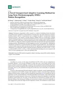
Fig. 1: Encoding of local descriptors to form a global representation which can be compared.

but use full document images which are created artificially by means of random segmented words from the original writing. In this way, they generated about 500 training and about twenty testing samples per writer to get more diverse feature vectors. The similarity is computed by means of the log-likelihood ratio of the CNN activation features of the penultimate layer. They presented the current best results on the CVL dataset and the second best results using the ICDAR13 dataset.

a possible normalization step, the global representations can be compared to each other. In case of image retrieval this is commonly done by means of the cosine distance between the global representations. 1) Aggregation: Sum pooling is the standard aggregation method for pooling local descriptors. Max pooling requires embedding functions that associate a certain strength to one visual word which is not directly applicable to the most common embedding techniques that rely on higher order statistics [15]. III. M ETHODOLOGY The drawback of sum pooling is that it assumes that the Commonly, encoding local descriptors is achieved by com- descriptors in an image are independently and identically puting statistics of a background model, such as k-means, distributed (iid). More frequently occurring descriptors will to embed each descriptor into a higher dimensional space, be more influential in the final representation, a. k. a. visual which are then aggregated. A popular encoding technique is burstiness. Thus, encoding methods have to normalize for this. VLAD [13], which aggregates first order statistics with sum In general, this is achieved during embedding or normalization. pooling. The global representation is typically compared using Alternatively, generalized max pooling (GMP) [17] and demothe cosine distance. cratic aggregation [14] were proposed to counter this in the In this work we investigate how VLAD encoding of CNN aggregation step. Both methods re-weight the patch statistics activations compares to the more recent triangulation embed- such that their influence regarding the final similarity score ding [14]. We further explore generalized max pooling [17], is equalized. Comparing both approaches [15], GMP showed which balances the embeddings with regard to the final superior performance. As indicated by its name, it generalizes similarity score. To the best of our knowledge this has not yet max pooling by formulating the balancing problem of any been explored for CNN activations. Additionally, we evaluate embedding φ(x) ∈ RD , x ∈ RDl as ridge regression problem. the effect of PCA whitening on the different parts of the Therefore, let [15] pipeline. Instead of using the cosine distance, we further φ(x)> ξgmp (X ) = C, ∀x ∈ X , (1) explore exemplar classifiers to learn a similarity between representations. where x is a local descriptor of the set of all local image descriptors X , ξgmp is the GMP representation and C is a constant which can be set arbitrarily since it has no influence Similar to our previous work [10], we use the activations when the representation is eventually ` -normalized. Equ. (1) 2 from the penultimate layer from a trained CNN as features. can be generalized for the D × n matrix Φ of all n patch The CNN is trained with four million raw (i. e. non-normalized) embeddings to 32 × 32 patches randomly sampled from the script contour. The Φ> ξgmp = 1n , (2) contours are obtained by a connected component analysis of the binarized images. We evaluate different network topologies where 1n denotes the vector of all constants set to 1. This to investigate their influence on the retrieval performance. linear system can be turned into a least-squares ridge regression The CNN activation features are then encoded to a global problem: representation. ξgmp = argminkΦ> ξ − 1n k2 + λkξk2 , (3) ξ B. Encoding A. Feature Extraction

Encoding consists of two steps, cf. Fig. 1: i) an embedding step where a, possible non-linear, function is applied to the local feature vectors in order to create a high dimensional representation, and ii) an aggregation step where the embedded local descriptors are pooled into a fixed-length vector. After

with λ being a regularization term that stabilizes the solution. Equ. (3) can be computed using conjugate gradient descent (CGD). In the remainder, ψ denotes the aggregated result. CGD can typically be applied component-wise, i. e., on each φk (see below), to speed up the process.

2) VLAD Embedding: VLAD can be viewed as a nonprobabilistic version of the Fisher Kernel [13] encoding only first order statistics. In combination with improvements such as whitening [18], intra-normalization [19], or residual normalization [20], VLAD is one of the standard encoding techniques. We successfully employed it for writer identification [21] and it has already been used in combination with deep-learning-based features for the task of classification and retrieval [22]–[24]. For VLAD encoding, the embedding function φ for the local descriptor x is computed by the residual to its nearest cluster center µk of the dictionary D = {µk ∈ RDl , k = 1, . . . , K}: φVLAD,k (x) = αk (x)(x − µk )  1 if k = argmin kx − µj k2 j=1,...,K αk (x) = . 0 else

(4) (5)

> > The full embedding follows as φVLAD = (φ> 1 , . . . , φK ) . VLAD encodings can be normalized to counter visual burstiness. The most popular normalization technique is power normalization, where each element ψi of the aggregated embedding ψ is normalized as:

ψˆi = sign(ψi )|ψi |p , ∀ψi ∈ ψ ,

(6)

where p is typically chosen to be 0.5. This is also known as signed square root (SSR), which resembles the Hellinger kernel. Power normalization is typically followed by an `2 normalization. Other proposed normalization techniques are residual normalization [20] and intra normalization [19]. In the former one, each embedding φk is `2 -normalized. In intra normalization, the component-wise aggregated embeddings ψk are `2 normalized. It is also beneficial to decorrelate and whiten the representations to prevent an over-counting of co-occurrences [18]. This is commonly achieved by means of a principal component analysis with whitening (PCA whitening). PCA whitening can be applied either at the global representation ψ or at the embeddings φ as well as their individual components ψk and φk , where the latter one was suggested by Delhumeau et al. [20] and referred to local coordinate systems (LCS). 3) Triangulation Embedding: Triangulation embedding [14] is very similar to VLAD with residual normalization. The normalized residuals of anchor points (= cluster centers) to feature descriptors are computed. These can be viewed as directions discarding absolute distances to cluster centers. The key difference is that no association function (α) is applied to the vectors. All normalized residuals are encoded, not just the nearest neighbor: xt − µk . (7) φT-Emb,k (xt ) = kxt − µk k2 Each embedding is whitened using PCA. However, instead of a dimensionality reduction, the authors proposed to discard the largest Dl eigenvalues and corresponding eigenvectors. This has the effect of reducing the variance of the cosine similarity between unrelated descriptors [14]. Each embedding is subsequently `2 -normalized and afterwards aggregated. Note,

due to the `2 normalization, the actual linear PCA whitening cannot be applied after the aggregation. In contrast to power normalization, the authors [14] suggested the use of rotation normalization where the aggregated embedding is first rotated by means of a PCA and then powernormalized. C. Exemplar Support Vector Machines Recently, we proposed the use of Exemplar SVMs (ESVM) in the context of writer recognition [25]. Since the training and test sets of common writer recognition datasets are disjoint, an end-to-end classification of the writers is not possible. However, this allows to compute probe individual classifiers. The encoding of each probe sample serves as single positive instance while all samples from the training set are the negative samples for a linear support vector machine. This can be interpreted as computing an individual similarity for each query document. For evaluation, each other document is ranked according to the score of the probe ESVM. IV. E VALUATION A. Datasets We evaluate the following publicly available datasets: • The ICDAR13 dataset [26] consists of four samples per writer, where each writer contributed two samples in English and two samples in Greek. The test set consists of 250 writers and the training set contains 100 writers. • The CVL dataset [27] (v. 1.1) contains 310 writers. 283 writers copied five texts (one in German and four in English). The remaining 27 writers contributed seven texts (one in German and six in English). We use the first five forms of all 310 writers as test set and all samples of the IAM dataset [28] for training. • The KHATT dataset [29] consists of 1000 writers, each contributing four documents written in Arabic. The dataset is divided into three disjoint, i. e., writer independent, sets for training (70 %), validation (15 %) and testing (15 %). The ICDAR13 and CVL datasets are text dependent, i. e., each writer copied the same four to seven forms. Conversely, two of the four forms of the KHATT dataset contain unique paragraphs. We binarized the IAM, CVL, and KHATT datasets using Otsu’s method [30] to be more similar to the ICDAR13 dataset and making them more independent of the pen used. The datasets are evaluated using a leave-one-sample-out cross validation. All results are given in terms of mean average precision (mAP), which computes the mean across the average precisions of all queries. The average precision of a query is computed by ranking the remaining documents according to their similarity to the query. Note, all values are shown in percent. B. CNN Activation Features We tested several architectures. First, we employ a four layer (not counting pooling layers) deep CNN denoted as LeNet, which we used in our previous work [10]. It has two convolutional layers, each followed by a max pooling layer,

100

LeNet (SGD) ResNet-8 (SGD) ResNet-22 (SGD)

Error [%]

90 80 70 60

TABLE II: Comparison of VLAD in combination with LCS with triangulation embedding (avg. of 5 runs, ICDAR13 test set). Method

mAP

VLAD + ResNorm + LCS wh. VLAD + ResNorm + LCS++ T-Emb T-Emb16

90.44 90.42 89.71 87.65

50 40

epochs using the proposed learning rate schedule. We also used the models after the fifth epoch for the ResNet models since Epochs the error stagnated at this point. Additionally, we evaluated the effect of decorrelating the activations by means of i) PCA Fig. 2: Test error of the different architectures using the ICDAR13 training data (subset). rotation and whitening and ii) zero component analysis (ZCA) with whitening. ZCA whitening rotates the data back to be as TABLE I: Evaluation of different decorrelation methods for CNN activation close to the input as possible. In the field of deep learning, features extracted from the script contour (mAP, avg. of 5 runs, ICDAR13 ZCA whitening is more common than PCA whitening. test set). For the baseline encoding, we employ VLAD encoding (note: Method Baseline PCA wh. ZCA wh. a pure sum pooling, i. e., no embedding, achieves 78.80 mAP). LeNet-A 86.75 88.50 87.21 Since VLAD encoding depends much on a good background LeNet-B 88.02 88.58 89.21 model, we compute five different VLAD-encodings and give ResNet-8 88.39 89.83 88.68 the average result. The background model is computed by ResNet-20 89.86 90.01 89.96 a mini-batch version of k-means [33] using different seeds and different selection of training samples. In this way, we have a large variability in the background models. The VLAD and a fully connected layer followed by the classification layer. encodings are individually normalized by power normalization (p = 0.5) followed by an `2 normalization. In addition to the LeNet architecture, we evaluate two Tab. I depicts all mAP results. The baseline results (first different residual network (ResNet) [31], [32] models of column) show that LeNet-A is inferior to LeNet-B, suggesting different depths. We follow the architectural design and training that a learning rate schedule is beneficial for the final feature procedure of He et al. [31] for the CIFAR10/100 datasets, representation. Any LeNet configuration performs worse than where we evaluated eight and twenty layers deep CNNs, further ResNets. A decorrelation is especially beneficial for the smaller denoted as ResNet-8 and ResNet-20. networks. However, no decorrelation method is significantly The networks are optimized using SGD w. r. t. the crosssuperior. Interestingly, a PCA whitening of the ResNet-20 entropy loss, a Nesterov momentum of 0.9 and a weight model achieves the highest average results. Exchanging SSR decay of 10−4 . We use an initial learning rate of 0.01 which with intra normalization [19] or residual normalization [20] is multiplied by 0.1 after three epochs and once more after for the baseline experiment performed worse with 89.44 and four epochs. The learning curves of the validation set (20 k 88.31 mAP, respectively (no normalization at all: 88.46 mAP). independent patches) for the first ten epochs can be seen in In the following experiments, we used the activation features Fig. 2. of the ResNet-20 model, if not mentioned otherwise in its Comparing the LeNet architecture with residual networks, non-whitened version. the plot clearly shows the advantage of the latter. The deeper ResNet reduced the error rate below 50 %. This means in more D. From VLAD to Triangulation Embedding than 50 % a 32 × 32 patch can be assigned to the correct Since triangulation embedding is an adapted VLAD enwriter. However note that a deeper network also needs a longer coding, it is interesting to explore the individual adjustments. training time. Instead of T-emb’s global PCA whitening, we use LCS [20] with whitening on `2 normalized residuals (VLAD + ResNorm C. Decorrelation of CNN Activations + LCS wh.). This is compared with a variant where the Given the trained models, we can use them as feature first component of each PCA transformed φk is discarded extractors by forwarding the contour patches of a query sample (VLAD + ResNorm + LCS++). Two variants of triangulation through the networks. In all cases we used the 64-dimensional embedding are used for comparison. The first one uses 100 activations of the penultimate layer as features. They are cluster centers similar to VLAD (T-Emb), and the other one subsequently `2 -normalized. For LeNet, we compared two uses 16 components (T-Emb16). The latter is the default value different variants: LeNet-A refers to the results using the very of triangulation embedding [14] to speed up the aggregation same LeNet model of our previous work [10], i. e., the model process. Tab. II shows that VLAD in combination with LCS after 20 epochs trained by a fixed learning rate of 0.01, while whitening is in average superior to triangulation embedding. LeNet-B denotes the results using the LeNet model after five This suggests that the power of triangulation is not based on 0

1

2

3

4

5

6

7

8

9

10

TABLE III: Evaluation of CNN activation features in combination with T-Emb (mAP, avg. of 5 runs, ICDAR13 test set). Method

VLAD++

T-Emb

T-Emb16

90.44 81.73 82.23 83.04

89.71 88.78 89.39 90.08

87.65 88.81 89.60 90.21

Baseline RotNorm PCA wh. joint PCA wh.

TABLE V: Evaluation of ESVMs using (a) different embeddings, aggregated with GMP and (b) additional PCA whitening of the CNN activation features (mAP, avg. of 5 runs, ICDAR13 test set). Method

Sum

GMPλ=1

GMPλ=103

VLAD++ T-Emb16

90.44 87.65

89.74 78.59

90.66 89.11

the aggregation of more descriptors but instead on the positive effect of PCA whitening. To make the evaluation process completely fair, we also evaluated the effect of rotation normalization (RotNorm), which was proposed in combination with triangulation embedding [14]. Additionally, we evaluated a simple PCA whitening (PCA wh.) and a joint PCA whitening (joint PCA wh.), where the encodings of the five runs are concatenated and jointly whitened. Tab. III shows that another decorrelation of the final aggregated embedding is not beneficial. While a joint PCA whitening shows some improvements for triangulation embedding, it worsens the results of VLAD plus residual normalization and LCS whitening (VLAD++). E. Sum Pooling vs. Generalized Max Pooling

ESVM

Baseline

ESVM

89.86 90.66 89.11

91.72 91.64 91.56

90.19 90.41 89.24

93.24 91.53 92.73

(a) CNN-AF

TABLE IV: Comparison of sum pooling and GMP (mAP, avg. of 5 runs, ICDAR13 test set). Method

Baseline

VLAD VLAD++ T-Emb16

(b) CNN-AF + PCA wh.

TABLE VI: Comparison with the state of the art. Method

Top-1

H-2

H-3

S-5

S-10

mAP

[12] [25]

99.0 99.7

84.4 84.8

68.1 63.5

99.2 99.8

99.6 99.8

– 89.4

VLAD VLAD + E

99.0 99.6

85.3 89.8

68.6 77.0

99.4 99.8

99.7 99.9

90.2 93.2

(a) ICDAR13 Method

Top-1

H-2

H-3

S-5

S-10

mAP

[12] [25]

99.7 99.2

99.0 98.4

97.9 97.1

99.8 99.6

100 99.7

– 98.0

VLAD VLAD + E

99.2 99.5

98.4 99.0

96.1 97.7

99.5 99.6

99.6 99.8

97.4 98.4

(b) CVL Method

Top-1

H-2

H-3

S-5

S-10

mAP

[25]

99.5

96.5

92.5

99.5

99.5

97.2

VLAD VLAD + E

99.1 99.6

93.8 97.6

88.2 94.5

99.4 99.7

99.6 99.7

95.5 98.0

(c) KHATT

The use of GMP requires the proper choice of the regularization parameter λ. Murray et al. [15] suggested that a factor of 1.0 works well in practice. However, cross-validating its G. Comparison with the State of the Art effect on the ICDAR13 training set showed that a much higher Finally, we compare the results with the state of the art on the value of λ = 1000 is preferable for the encodings used. ICDAR13, CVL, and KHATT datasets. Additional to the mAP, In Tab. IV, we compare sum pooling with GMP using the we depict the following common writer identification / retrieval two embeddings VLAD++ and T-Emb with 16 components measures: Top-1 gives the probability that the first retrieved (T-Emb16). When using a proper regularization parameter, result stems from the same writer. While Soft-5 (S-5) / Soft-10 GMP outperforms sum pooling by a small factor. However, (S-10) requires that one of the top five / ten results is written the benefit is small and another parameter (λ) needs to be by the query writer, Hard-2 (H-2) / Hard-3 (H-3) requires that cross-validated. all two / three top ranked results are from the same writer. F. Exemplar Support Vector Machines and PCA whitening We used VLAD in combination with generalized max pooling (λ = 1000) and SSR. Additionally, we show the We compare the effectiveness of ESVMs with: VLAD plus results with the Exemplar SVM step. We compare our results SSR (VLAD), VLAD with LCS whitening (VLAD++) and triangulation embedding (T-Emb16). All methods use GMP with our previous work [25] and the work of Tan and Wu [12]. (λ = 1000), the margin parameter of the SVM is for each To the best of our knowledge, these two methods are currently method cross-validated using the training set. Comparing the leading the ICDAR13, CVL and KHATT datasets. Tab. VI shows all results. Our method achieves results similar different results of Tab. Va, we see that all methods perform well. Interestingly, the basic VLAD method performs the best. to the state of the art on all datasets while even being superior Hence, we can conclude that the additional decorrelation with on the ICDAR13 and KHATT dataset. Previous evaluations on PCA, which is part of LCS and triangulation embedding does the CVL dataset [25] suggest that a better background model not necessarily improve the recognition results. Additionally, could further improve the results for this dataset. we investigated the effect of the PCA whitened version of the V. C ONCLUSION CNN activation features. Tab. Vb shows that this step improves the recognition of the basic VLAD method and triangulation In this work, we evaluated several effects related to the embedding. encoding of local descriptors. We showed that 1) a deeper

CNN only slightly achieves higher retrieval performance. 2) Triangulation embedding is not better than VLAD when either the local descriptors or the embeddings are decorrelated by means of a PCA whitening. 3) Generalized max pooling is slightly better than sum pooling but is sensitive to a proper regularization. 4) When using Exemplar SVMs, all three methods perform similarly well, where VLAD in combination with power normalization performs slightly better. The proposed combination of deep CNN activation features, VLAD encoding, normalization and Exemplar SVMs is similar or better than state-of-the-art methods on three publicly available datasets. For future work, we would like to explore different layers than the penultimate layer for feature extraction. Furthermore, larger input patch sizes could also be beneficial. R EFERENCES [1] A. Brink, J. Smit, M. Bulacu, and L. Schomaker, “Writer Identification Using Directional Ink-Trace Width Measurements,” Pattern Recognition, vol. 45, no. 1, pp. 162–171, 2012. 1 [2] T. Gilliam, R. C. Wilson, and J. A. Clark, “Scribe Identification in Medieval English Manuscripts,” in 20th International Conference on Pattern Recognition (ICPR), 2010, pp. 1880–1883. 1 [3] D. Fecker, A. Asit, V. Margner, J. El-Sana, T. Fingscheidt, V. M¨argner, J. El-Sana, and T. Fingscheidt, “Writer Identification for Historical Arabic Documents,” in 2014 22nd International Conference on Pattern Recognition (ICPR), 2014, pp. 3050–3055. 1 [4] S. He and L. Schomaker, “Delta-n Hinge: Rotation-Invariant Features for Writer Identification,” in 2014 22nd International Conference on Pattern Recognition (ICPR), 2014, pp. 2023–2028. 1 [5] A. Krizhevsky, I. Sutskever, and G. E. Hinton, “ImageNet Classification with Deep Convolutional Neural Networks,” in Advances In Neural Information Processing Systems 25. Curran Associates, Inc., 2012, pp. 1097—-1105. 1 [6] T. Bluche, H. Ney, and C. Kermorvant, “Feature Extraction with Convolutional Neural Networks for Handwritten Word Recognition,” in 2013 12th International Conference on Document Analysis and Recognition, 2013, pp. 285–289. 1 [7] M. Jaderberg, A. Vedaldi, and A. Zisserman, “Deep Features for Text Spotting,” in Computer Vision – ECCV 2014. Springer International Publishing, 2014, vol. 8692, pp. 512–528. 1 [8] F. Wahlberg, T. Wilkinson, and A. Brun, “Historical Manuscript Production Date Estimation Using Deep Convolutional Neural Networks,” in 2016 15th International Conference on Frontiers in Handwriting Recognition (ICFHR), 2016, pp. 205–210. 1 [9] S. Fiel and R. Sablatnig, “Writer Identification and Retrieval Using a Convolutional Neural Network,” in Computer Analysis of Images and Patterns: 16th International Conference, CAIP 2015, Valletta, Malta, September 2-4, 2015, Proceedings, Part II, G. Azzopardi and N. Petkov, Eds. Springer International Publishing, 2015, pp. 26–37. 1 [10] V. Christlein, D. Bernecker, A. Maier, and E. Angelopoulou, “Offline Writer Identification Using Convolutional Neural Network Activation Features,” in Pattern Recognition: 37th German Conference, GCPR 2015, Aachen, Germany, October 7-10, 2015, Proceedings, J. Gall, P. Gehler, and B. Leibe, Eds. Springer International Publishing, 2015, vol. 9358, pp. 540–552. 1, 2, 3, 4 [11] L. Xing and Y. Qiao, “DeepWriter: A Multi-Stream Deep CNN for Textindependent Writer Identification,” in 2016 15th International Conference on Frontiers in Handwriting Recognition (ICFHR), 2016, pp. 584–589. 1 [12] Y. Tang and X. Wu, “Text-Independent Writer Identification via CNN Features and Joint Bayesian,” in 2016 15th International Conference on Frontiers in Handwriting Recognition (ICFHR), 2016, pp. 566–571. 1, 5 [13] H. J´egou, F. Perronnin, M. Douze, J. S´anchez, P. P´erez, and C. Schmid, “Aggregating Local Image Descriptors into Compact Codes,” IEEE Transactions on Pattern Analysis and Machine Intelligence, vol. 34, no. 9, pp. 1704–1716, 2012. 1, 2, 3

[14] H. J´egou and A. Zisserman, “Triangulation Embedding and Democratic Aggregation for Image Search,” in 2014 IEEE Conference on Computer Vision and Pattern Recognition (CVPR), 2014, pp. 3310–3317. 1, 2, 3, 4, 5 [15] N. Murray, H. Jegou, F. Perronnin, and A. Zisserman, “Interferences in Match Kernels,” IEEE Transactions on Pattern Analysis and Machine Intelligence, vol. PP, no. 99, p. 1, 2016. 1, 2, 5 [16] T. Hoang, T.-T. Do, D.-K. L. Tan, and N.-M. Cheung, “Selective Deep Convolutional Features for Image Retrieval,” in ACM Multimedia conference, 2017. 1 [17] N. Murray and F. Perronnin, “Generalized Max Pooling,” in 2014 IEEE Conference on Computer Vision and Pattern Recognition, 2014, pp. 2473–2480. 1, 2 [18] H. J´egou and C. Ondˇrej, “Negative Evidences and Co-occurences in Image Retrieval: The Benefit of PCA and Whitening,” in Computer Vision – ECCV 2012: 12th European Conference on Computer Vision, Florence, Italy, October 7-13, 2012, Proceedings, Part II, A. Fitzgibbon, S. Lazebnik, P. Perona, Y. Sato, and C. Schmid, Eds. Springer Berlin Heidelberg, 2012, pp. 774–787. 3 [19] R. Arandjelovic and A. Zisserman, “All About VLAD,” in 2013 IEEE Conference on Computer Vision and Pattern Recognition (CVPR), 2013, pp. 1578 – 1585. 3, 4 [20] J. Delhumeau, P.-H. Gosselin, H. J´egou, and P. P´erez, “Revisiting the VLAD Image Representation,” in 21st ACM International Conference on Multimedia - MM ’13. ACM, 2013, pp. 653–656. 3, 4 [21] V. Christlein, D. Bernecker, and E. Angelopoulou, “Writer Identification using VLAD Encoded Contour-Zernike Moments,” in 2015 13th International Conference on Document Analysis and Recognition (ICDAR), 2015, pp. 906–910. 3 [22] Y. Gong, L. Wang, R. Guo, and S. Lazebnik, “Multi-scale Orderless Pooling of Deep Convolutional Activation Features,” in Computer Vision – ECCV 2014, D. Fleet, T. Pajdla, B. Schiele, and T. Tuytelaars, Eds. Springer International Publishing, 2014, vol. 8695, pp. 392–407. 3 [23] J. Y. H. Ng, F. Yang, and L. S. Davis, “Exploiting Local Features from Deep Networks for Image Retrieval,” in 2015 IEEE Computer Society Conference on Computer Vision and Pattern Recognition Workshops (CVPRW), 2015, pp. 53–61. 3 [24] M. Paulin, J. Mairal, M. Douze, Z. Harchaoui, F. Perronnin, and C. Schmid, “Convolutional Patch Representations for Image Retrieval: An Unsupervised Approach,” International Journal of Computer Vision, vol. 121, no. 1, pp. 149–168, 2016. 3 [25] V. Christlein, D. Bernecker, F. H¨onig, A. Maier, and E. Angelopoulou, “Writer Identification Using GMM Supervectors and Exemplar-SVMs,” Pattern Recognition, vol. 63, pp. 258–267, 2017. 3, 5 [26] G. Louloudis, B. Gatos, N. Stamatopoulos, and A. Papandreou, “ICDAR 2013 Competition on Writer Identification,” in 2013 12th International Conference on Document Analysis and Recognition (ICDAR), 2013, pp. 1397–1401. 3 [27] F. Kleber, S. Fiel, M. M. Diem, and R. Sablatnig, “CVL-DataBase: An Off-Line Database for Writer Retrieval, Writer Identification and Word Spotting,” in 2013 12th International Conference on Document Analysis and Recognition (ICDAR), 2013, pp. 560 – 564. 3 [28] U.-V. Marti and H. Bunke, “The IAM-Database: An English Sentence Database for Offline Handwriting Recognition,” International Journal on Document Analysis and Recognition, vol. 5, pp. 39–46, 2002. 3 [29] S. A. Mahmoud, I. Ahmad, W. G. Al-Khatib, M. Alshayeb, M. Tanvir Parvez, V. M¨argner, and G. A. Fink, “KHATT: An Open Arabic Offline Handwritten Text Database,” Pattern Recognition, vol. 47, no. 3, pp. 1096–1112, 2014. 3 [30] N. Otsu, “A Threshold Selection Method from Gray-Level Histograms,” Systems, Man, and Cybernetics, IEEE Transactions on, vol. 9, no. 1, pp. 62–66, 1979. 3 [31] K. He, X. Zhang, S. Ren, and J. Sun, “Deep Residual Learning for Image Recognition,” in 2016 IEEE Conference on Computer Vision and Pattern Recognition (CVPR), 2016, pp. 770–778. 4 [32] ——, “Identity Mappings in Deep Residual Networks,” in Computer Vision – ECCV 2016: 14th European Conference, Amsterdam, The Netherlands, October 11–14, 2016, Proceedings, Part IV, B. Leibe, J. Matas, N. Sebe, and M. Welling, Eds. Springer International Publishing, 2016, pp. 630–645. 4 [33] D. Sculley, “Web-Scale K-means Clustering,” in 19th International Conference on World Wide Web, ser. WWW ’10. ACM, 2010, pp. 1177–1178. 4